Báo cáo hóa học: " Research Article Reverse Smoothing Effects, Fine Asymptotics, and Harnack Inequalities for Fast Diffusion Equations" pptx

Hindawi Publishing Corporation
Boundary Value Problems
Volume 2007, Article ID 21425, 31 pages
doi:10.1155/2007/21425
Research Article
Reverse Smoothing Effects, Fine Asymptotics, and Harnack
Inequalities for Fast Diffusion Equations
Matteo Bonforte and Juan Luis Vazquez
Received 30 June 2006; Accepted 20 September 2006
Recommended by Vincenzo Vespri
We investigate local and global properties of positive solutions to the fast diffusion equa-
tion u
t
= Δu
m
in the good exponent range (d − 2)
+
/d < m < 1, corresponding to general
nonnegative initial data. For the Cauchy problem posed in the whole Euclidean space
R
d
,
we prove sharp local positivity estimates (weak Harnack inequalities) and elliptic Har-
nack inequalities; also a slight improvement of the intrinsic Harnack inequality is given.
We use them to derive sharp global positivity estimates and a global Harnack principle.
Consequences of these latter estimates in terms of fine asymptotics are shown. For the
mixed initial and boundary value problem posed in a bounded domain of
R
d
with homo-
geneous Dirichlet condition, we prove weak, intrinsic, and elliptic Harnack inequalities

for intermediate times. We also prove elliptic Harnack inequalities near the extinction
time, as a consequence of the study of the fine asymptotic behavior near the finite extinc-
tion time.
Copyright © 2007 M. Bonforte and J. L. Vazquez. This is an open access article distrib-
uted under the Creative Commons Attribution License, which permits unrestricted use,
distribution, and reproduction in any medium, provided the original work is properly
cited.
1. Introduction
In this paper, we are interested in the questions of boundedness, positivity, and regularity
of the solutions of fast diffusion equations. Though the arguments have a more general
scope, two settings will be considered in order to obtain sharp results: in one of them, the
Cauchy problem is considered in the whole space
u
t
= Δ

u
m

in Q = (0,+∞) ×R
d
,
u(0,x)
= u
0
(x)inR
d
,
(1.1)
2 Boundary Value Problems

and in the range (d
− 2)
+
/d = m
c
<m<1. In the second option, the mixed Cauchy-
Dirichlet problem is considered in bounded domains with smooth boundary
u
t
= Δ

u
m

in Q = (0,+∞) ×Ω,
u(0,x)
= u
0
(x)inΩ,
u(t,x)
= 0fort>0, x ∈ ∂Ω,
(1.2)
and in the range (d
− 2)
+
/(d +2)= m
s
<m<1. In both cases, nonnegative solutions are
considered. The restrictions on the exponent range are not a matter of convenience.
It is well known that the solutions of the heat equation u

t
= Δu posed in the whole
space with nonnegative data at t
= 0 become p ositive and smooth for all positive t imes
and all points of space. The same positivity propert y is true in many other settings, for ex-
ample, for nonnegative solutions posed in a bounded space domain with zero boundary
conditions. Such properties of positivity and smoothness are shared by the fast diffusion
equation
u
t
= Δu
m
,0<m<1, (1.3)
but this happens under certain conditions on the exponent and data and with quite dif-
ferent quantitative estimates.
The question of boundedness is closely related to existence theory and has been much
investigated in the whole exponent range m
∈ R. A comprehensive account can be found
in works of one of the authors (see [1–3]). The smoothing effect explained there is usually
expressed in the form


u(t)


∞
≤
C



u
0


σ
1
t
α
, (1.4)
where t>0andalltheL
p
are taken over the whole domain Ω or R
d
. The positive constants
C, σ,andα depend only on m, d. The analysis shows that the FDE maps initial data,
possibly unbounded, to bounded solutions if m is larger than a first-critical exponent
m
c
= (d − 2)
+
/d. The situation becomes quite involved, and interesting, for subcritical m.
A natural problem that we will address here arises next: starting from nonnegative ini-
tial data, do we obtain strictly positive solut ions, at least locally? This positivity property
is strictly related to Harnack inequalities, as we will see. If we express the positivity re-
sult in terms of L
p
norms, we are led to the case of negative exponents and of course the
quantities
 f 
−p

=


Ω
f (x)
−p
dx

−1/p
(1.5)
M. Bonforte and J. L. Vazquez 3
are no more norms in the usual sense. But there is a nice well-known result, which helps
us to better understand the nature of such lower bounds:
inf
x∈Ω


f (x)


=
f 
−∞
= lim
p→∞
 f 
−p
. (1.6)
The aim of this paper is to present from a unified point of view some results and
techniques recently discovered by the authors and described in whole detail in [4, 5],

and also to discuss some new ideas to attack some open problems related to Harnack
inequalities. Let us present the lower bounds that we obtain. We take the case of the
Cauchy problem posed in the whole space: in Theorem 2.1,weprovethat
inf
x∈B
R
(x
0
)
u(t,x) ≥ M
R

x
0

H

t
t
c

> 0. (1.7)
Here,
M
R
(x
0
) is the average initial mass in the ball B
R
(x

0
), H is an explicit function of
time relative to the characteristic time t
c
, which is loosely speaking, a time that we have to
wait in order to let the regularization to take place, and is calculated in terms of the initial
data. For t
≥ t
c
, the above lower bound can be rewritten as


u(t)


L
−∞
(B
R
(x
0
))
≥ K
m,d


u
0



2ϑ
L
1
(B
R
(x
0
))
t
−dϑ
, (1.8)
that is, exactly the reverse of the standard smoothing effect above, thought as L
1
–L
∞
reg-
ularization, and expressed as a local L
1
–L
−∞
smoothing effect (over balls); for this reason,
we call it revers e smoothing effect.
Putting together the direct and reverse smoothing effects, we obtain the intrinsic and
elliptic Harnack inequalities and thus as a consequence, we have a quite simple proof of
the H
¨
older continuity of the solution, which has been first proved by DiBenedetto et al.,
see, for example, [6, 7], by entirely different techniques.
When dealing with elliptic problems, our positivity result, or reverse smoothing effect,
is also known as weak Harnack inequality or half Harnack. Indeed, nothing is more natu-

ral than this terminology since this easily implies intrinsic Harnack inequality as a corol-
lary, compare Theorems 6.2 and 6.4. Moreover, the combination of direct and reverse
smoothing effects implies a Harnack inequality of elliptic type, compare Theorems 6.1
and 6.5, namely, we compare the supremum and infimum of the solution at the same
time.
Another issue that we address is the extension to the whole space (or domain) of local
positivity properties. This leads to the global Harnack principle, GHP, that is, to accu-
rate upper and lower bounds in terms of some special (sub/super) solutions. In the case
of the whole space, the super- and subsolutions are Barenblatt functions. In the case of
bounded domains, the global Harnack principle was first proved in [7], and the super-
and subsolutions were related to the solution obtained by separation of variables.
We also investigate the connection between the global Harnack principle and the fine
asymptotic behavior, first introduced by one of the authors in [1], in terms of uniform
convergence in relative error, shortly CRE. We show that the GHP implies CRE both in
thecaseof
R
d
and in the case of bounded domains.
4 Boundary Value Problems
Finally, we show in the case of bounded domains that the convergence in relative error
implies elliptic Harnack inequalities for times near the extinction time, thus completing
the panorama of the validity of Harnack inequalities in the case of bounded domains.
Open problems. These ideas lead to further possible interesting generalizations which are
actually under investigation. For example, we can consider the case in w hich the problem
is posed on a Riemannian manifold, and the operator is the Laplace-Beltrami operator,
or when it is replaced by a more general elliptic operator, possibly with measurable coef-
ficients. The methods we present here may open new directions to solve the problem of
Harnack inequalities for more general nonlinear diffusion equations for a larger range of
exponents m.
Notation. In the sequel, the letters a

i
, b
i
, C
i
, K, k
i
, λ
i
, μ are used to denote universal
positive constants that depend only on m and d. The constant ϑ is fixed to the value
ϑ
= 1/(2 − d(1 − m)) > 0.
2.Positivityresultsforthefastdiffusion equation
We start our analysis by considering the problem of estimating the positivity of solutions
of the FDE, both in the case of the Cauchy problem posed in the whole
R
d
space and in
the case of the mixed Cauchy-Dirichlet problem posed in a domain of
R
d
. In both cases,
we analyze local and global positivity estimates. In view of the remarks of the introduc-
tion, the local positivity estimates can be considered as a reverse smoothing effect and
are independent of the choice of some explicit (sub-/super-) solutions. Vice versa, when
we deal with global positivity, we make use of some special (sub-/super-) solutions. For a
complete discussion of these results, we refer to our paper [5].
2.1. Local and global positivity estimates in
R

d
. Let us prove quantitative positivity es-
timates for the Cauchy problem posed in the whole Euclidean space
R
d
:
u
t
= Δ

u
m

in Q = (0,+∞) ×R
d
,
u(0,x)
= u
0
(x)inR
d
,
(2.1)
in the range (d
− 2)
+
/d = m
c
<m<1. We then derive elliptic Harnack inequalities. In the
results, we fix a point x

0
∈ R
d
and consider different balls B
R
= B
R
(x
0
)withR>0. We
introduce the following measures of the local mass:
M
R

x
0

=

B
R
u
0
(x) dx, M
R

x
0

=

M
R
R
d
. (2.2)
More precisely, we should write M
R
(u
0
,x
0
), M
R
(u
0
,x
0
), but we will even drop the variable
x
0
when no confusion is feared. This is the intrinsic positivity result that shows in a quan-
titative way that solutions are positive for all (x,t)
∈ Q. This type of results is also called
weak Harnack inequality,andalsohalf Harnack inequality or lower Harnack inequality,
meaning that it is half of the full pointwise comparison that Harnack inequalities imply.
M. Bonforte and J. L. Vazquez 5
1.2
1
0.8
0.6

0.4
0.2
0
0.511.522.53
t
H(t)
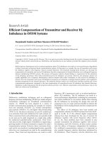
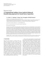
Figure 2.1. Approximative graphic of the functions u(t,x) (dotted line) and H(t) (solid line).
Theorem 2.1 (local positivity on R
d
). There ex ists a positive function H(t) such that for
any t>0 and R>0 the following bound holds true for all continuous nonnegative solutions
u to (2.1)withm
c
<m<1:
inf
x∈B
R
(x
0
)
u(t,x) ≥ M
R

x
0

H

t
t

c

. (2.3)
Function H(η) is positive and takes the precise form
H(η)
=
⎧
⎨
⎩
Kη
−dϑ
for η ≥ 1,
Kη
1/(1−m)
for η ≤ 1.
(2.4)
The characteristic time is given by
t
c
= CM
1−m
R
R
1/ϑ
. (2.5)
Constants C,K>0 depend only on m and d.
Figure 2.1 gives an idea of the positivity result, in particular the change of the behavior
of the general lower profile as a function of time. It shows the importance of the critical
time t
c

. For the sake of simplicity, we consider t
c
= 1.
Proof. We skip the proof of this result, given in [5], since it is similar to the proof of
the problem posed in a bounded domain, that we will present in Theorem 2.5;thatcase
which presents the extra difficulty caused by the phenomenon of extinction in finite time.
Instead, we concentrate on a number of observations.

(1) Characteristic time. Notice that t
c
is an increasing function of M
R
and R. This is in
contrast with the porous medium case m>1 where it can b e shown that t
c
decreases with
M
R
(see, e.g., [8]or[3, Chapter 4]).
(2) Minimax problem. Supposethatwewanttoobtainthebestofthelowerbounds
when t varies. This happens for t/t
c
≈ 1 and the value is
u

t
c
,0

≥

C
3
M
R
R
−d
, (2.6)
which is just proportional to the average. At this time also the maximum is controlled by
the average (see the upper estimate).
6 Boundary Value Problems
(3) The behavior of H is optimal in the limits t
 1andt ≈ 0 as the Barenblatt so-
lutions show. If we perform the explicit computation for the Barenblatt solution in the
worstcasewherethemassisplacedontheborderoftheballB
R
0
, it gives (see (2.8))
Ꮾ(0,t)
=
M
2ϑ
R
t
1/(1−m)

b
1
t
2ϑ
+ b

2
t
2ϑ
c

1/(1−m)
. (2.7)
The consideration of the Barenblatt solutions as an example leads us to examine what
is the form of the positivity estimate when we move far away from a ball in space. Indeed,
we can get a global estimate by carefully inserting a Barenblatt solution with small mass
below our solution. Let us recall that the Barenblatt solution of mass M is given by the
formula
Ꮾ(t,x;M)
=
t
1/(1−m)

b
1
t
2ϑ
/M
2ϑ(1−m)
+ b
2
|x|
2

1/(1−m)
, (2.8)

and also that
t
c
= CM
(1−m)
R
R
1/ϑ
. (2.9)
The following theorem can be viewed as a weak global Harnack principle, since it leads
to the global Harnack principle, which will be derived in the next section. Notice that the
parameters of the Barenblatt subsolution have a different form in the two cases t
≥ t
c
and
0 <t<t
c
.
Theorem 2.2 (global positivity in
R
d
). (I) There exist τ
1
∈ (0,t
c
) and M
c
> 0 such that for
all x
∈ R

d
and t ≥ t
c
,
u(t,x)
≥ Ꮾ

t − τ
1
,x;M
c

, (2.10)
where τ
1
= λt
c
and M
c
= kM
R
for some universal constants λ,k>0 which depend only on m
and d. (II) For any 0 <ε<t
c
, the global lower bound is valid for t ≥ ε,
u(t,x)
≥ Ꮾ

t − τ(ε),x;M(ε)


, (2.11)
with τ(ε)
= λε and
M(ε)
=

ε
t
c

1/(1−m)
M
c
= k
1

ε
R
1/ϑ

1/(1−m)
. (2.12)
Proof. The proof presented here has been taken from [5]. The main result is the first, the
point of stating (II) is to have an estimate for small times (w ith a smaller time shift) at the
price of having a subsolution with smaller mass. Let us point out that the last constant
k
1
= kC
−1/(1−m)
. We divide the proof in a number of steps; the proof of (I) consists of

steps (i)–(iii). (i) Let us first argue for x
∈ B
R
(0) at time t = t
c
. As a consequence of our
local estimate (2.1)att
= t
c
, one gets
u

t
c
,x

≥
K
M
R
R
d
(2.13)
M. Bonforte and J. L. Vazquez 7
for all
|x|≤R.Hence,(2.10) is implied in this region by the inequality
K
M
R
R

d
≥ Ꮾ

t
c
− τ
1
,x;M
c

=

t
c
− τ
1

1/(1−m)

b
1

t
c
− τ
1

2ϑ
/M
2ϑ(1−m)

c
+ b
2
|x|
2

1/(1−m)
. (2.14)
Now we choose τ
1
= λt
c
with a certain λ ∈ (0,1). We put μ = 1 −λ ∈ (0,1) so that t
c
− τ
1
=
μt
c
. With this choice, (2.14)isequivalentto
b
1

μt
c

2ϑ
M
2ϑ(1−m)
c

+ b
2
|x|
2
≥
R
d(1−m)
μt
c
M
1−m
R
K
1−m
(2.15)
putting x
= 0 and using the value of t
c
, it is implied by the condition
M
c
= kM
R
, k ≤ b
1/(2ϑ(1−m))
1
K
1/2ϑ
(μC)
d/2

. (2.16)
(ii) We now extend the comparison to the region
|x|≥R,againattimet = t
c
.Wetake
as a domain of comparison the exterior space-time domain
S
=

τ
1
,t
c

×

x ∈ R
d
: |x| >R

. (2.17)
Both functions in estimate (2.10) are solutions of the same equation, hence we need only
to compare them on the parabolic boundary. Comparison at the initial time t
= τ
1
is clear
since B(t
c
− τ
1

,x;M
c
) vanishes. The comparison on the lateral boundary where |x|=R
and τ
1
≤ t ≤ t
c
amounts to
K
M
R
R
d

t
t
c

1/(1−m)
≥

t − τ
1

1/(1−m)

b
1

t − τ

1

2ϑ
/M
2ϑ(1−m)
c
+ b
2
R
2

1/(1−m)
. (2.18)
Raising to the power (1
− m) and using the value of t
c
,weget
K
1−m
t
R
2
C
≥
t − τ
1
b
1

t − τ

1

2ϑ
/M
2ϑ(1−m)
c
+ b
2
R
2
, (2.19)
or
K
1−m
b
1

t − τ
1

2ϑ
M
2ϑ(1−m)
c
+ K
1−m
b
2
R
2

≥

1 −
τ
1
t

R
2
C. (2.20)
If we have fixed τ
1
as before and if we define M
c
= kM
R
with k = k(m,d) small enough,
this inequality is true for τ
1
≤ t ≤ t
c
. (iii) Using now the maximum principle in S,the
proof of (2.10)isthuscompletefort
= t
c
in the exterior region. Since the comparison
holds in the interior region by step (i), we get a global estimate at t
= t
c
.(iv)Wenow

prove part (II) of the theorem. We only need to prove it at t
= ε.Werecallthatλ and M
c
are as defined in part (I). We know that
t
c
− τ
1
= μt
c
,withμ ∈ (0,1). (2.21)
8 Boundary Value Problems
Using the B
´
enilan-Crandall estimate, we have for 0 <t<t
c
u(t,x) ≥ u

t
c
,x

t
1/(1−m)
t
1/(1−m)
c
, (2.22)
together with the above estimate (2.10), we can see that
u(t,x)

≥ u

t
c
,x

t
1/(1−m)
t
1/(1−m)
c
≥
t
1/(1−m)
t
1/(1−m)
c
Ꮾ

t
c
− τ
1
,x;M
c

=
t
1/(1−m)
t

1/(1−m)
c

μt
c

1/(1−m)

b
1

μt
c

2ϑ
/M
2ϑ(1−m)
c
+ b
2
|x|
2

1/(1−m)
=
(μt)
1/(1−m)

b
1

(μt)
2ϑ
/M
2ϑ(1−m)
c
t
2ϑ
t
−2ϑ
c
+ b
2
|x|
2

1/(1−m)
= Ꮾ

μt,x;
M
c
t
1/(1−m)
t
1/(1−m)
c

=
Ꮾ


t − τ,x;M
c
(t)

(2.23)
once one lets t
− τ = μt and M
c
as above. The proof of (2.11)isthuscomplete. 
A consequence of this result is the fol low i ng lower asymptotic behavior that is peculiar
of the FDE evolution.
Corollary 2.3. Under the same hypothesis of Theorem 2.2,
liminf
|x|→∞
u(t,x)|x|
2/(1−m)
≥ c(m, d)t
1/(1−m)
. (2.24)
The constant c(m,d)
= (2m/ϑ(1 − m))
1/(1−m)
of the Barenblatt solution is sharp.
This result has been proved by Herrero and Pierre (see [9, Theorem 2.4]) by similar
methods. Here, it easily follows from the estimates of Theorem 2.2 which provides an
exact lower bound for al l times, not only for large times.
Remarks 2.4. (1) In order to complement the previous lower estimates, let us review what
is known about estimates from above. These depend on the behavior of the initial data
as
|x|→∞. Recall only that constant data produce the constant solution that does not

decay. Under the decay assumption on the initial datum u
0
∈ L
1
loc
(R
d
)

|y−x|≤|x|/2


u
0
(y)


dy = O

|
x|
d−2/(1−m)

as |x|−→∞, (2.25)
it has been proved by entirely different methods in [1]that
lim
|x|→∞
u(t,x)|x|
2/(1−m)
≤ c(m, d)(t + S)

1/(1−m)
, (2.26)
where S>0dependsontheconstantinthebound(2.25)as
|x|→∞. The time shift S is
needed in the asymptotic behavior of u as
|x|→∞. Actually, when the initial datum has
M. Bonforte and J. L. Vazquez 9
an exact decay at infinity, u
0
∼ a|x|
−2/(1−m)
,wehavemore
lim
|x|→∞
u(t,x)|x|
2/(1−m)
= C(t + S)
1/(1−m)
, (2.27)
with C
= 2m/ϑ(1 − m)andS = a
1−m
/C, and this cannot be improved as the delayed
Barenblatt solutions show. Moreover, t here exists a t
0
such that u
1−m
is convex as a func-
tion of x for t>t
0

,compare[10].
(2) In comparison with the upper bounds, we have shown that global lower estimates
need a time shift τ (in the other direction, explicitly calculated), but in the limit we can
put τ
= 0, as one can see above. Moreover, the behavior at infinity is independent of
the mass (a fact that is false for the heat equation), hence all Barenblatt solutions with
different free constant b
1
behave in the same way in the limit as |x|→∞,compare[1].
(3) We can also get better results if we consider radially symmetric initial data (always
in our range of parameters m
c
<m<1), compare [11].
2.2. Local and global positivity estimates on domains. In this section, we will prove
local positivity estimates (weak Harnack) and elliptic Harnack inequalities for the fast
diffusion equation in the range (d
− 2)
+
/d = m
c
<m<1inaEuclideandomainΩ ⊂ R
d
,
u
t
= Δ

u
m


in Q = (0,+∞) ×Ω,
u(0,x)
= u
0
(x)inΩ,
u(t,x)
= 0fort>0, x ∈ ∂Ω,
(2.28)
where Ω
⊂ R
d
is an open-connected domain with sufficiently smooth boundary. Since
we are interested in lower estimates, by comparison, we may assume that Ω is bounded
without loss of generality. In the case of bounded domains, an extra difficulty appears: the
extinction in finite time, for example, there exists a time T>0suchthatu(t,x)
≡ 0forany
t
≥ T and x ∈ Ω.IntheproofofTheorem 2.5, we prove a lower bound for such extinction
time in terms of the volume of the domain. This will in part icular show that in the case
of the whole
R
d
, solutions do not extinguish in finite time. This is the intrinsic positiv ity
result that shows in a quantitative way that solutions are positive for all (x,t)
∈ Q.Inthe
result, we fix a point x
0
∈ Ω and consider different balls B
R
= B

R
(x
0
)withR>0, included
in Ω. It is a version of Theorem 2.1 in the case of the mixed Cauchy-Dirichlet problem on
domains.
Theorem 2.5 (local positivity on domains). Let u be a continuous nonnegative solution to
(2.28), with m
c
<m<1. There exist times 0 <t
∗
c
<T
c
≤ T,whereT is the finite extinction
time, and a positive function H(t) such that for any t
∈ (0,T
c
) and R>0 such that
R
≤ Λ dist

x
0
,∂Ω

, (2.29)
the following bound holds true:
inf
x∈B

R
u(t,x) ≥ M
R
H

t
t
∗
c

, (2.30)
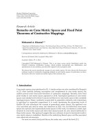
10 Boundary Value Problems
1.2
1
0.8
0.6
0.4
0.2
0
0.511.522.53
t
H(t)
Figure 2.2. Approximative graphic of the functions u(t,x) (dotted line) and H(t) (solid line).
where M
R
= M
R
/R
d
, M

R
=

B
R
u
0
(x) dx.FunctionH(t) is positive and takes the precise form
H(η)
=
⎧
⎪
⎨
⎪
⎩
Kη
−dϑ
for 1 ≤ η ≤
T
c
t
∗
c
,
Kη
1/(1−m)
for η ≤ 1.
(2.31)
The times 0 <t
∗

c
≤ T
c
≤ T are given by
t
∗
c
= τ
c
(2R)
1/dϑ
M
1−m
R
,
T
c
= τ

c

dist

x
0
,∂Ω

−
2R


M
1−m
R
.
(2.32)
Constants C, K, τ
c
, τ

c
, Λ > 0 depend only on d and m.
Figure 2.2 gives an idea of the positivity result, in particular the change of the behavior
of the general lower profile, in function of time, showing the importance of both the lower
critical time t
c
and the upper critical time T
c
. For the sake of simplicity, we consider t
c
= 1
and T
c
= 2.5, while the extinction time is taken as T = 3.
Proof. The proof presented here has been taken from [5]. It is a combination of several
steps. Without loss of generality, we assume that x
0
= 0. Different positive constants that
depend on m and d are denoted by C
i
. The precise values we get for C, K, τ

c
, τ

c
,andΛ
are given at the end of the proof.
Reduction. By comparison, we may assume that supp(u
0
) ⊂ B
R
(0). Indeed, a general
u
0
≥ 0 is greater than u
0
η, η being a suitable cutoff function compactly supported in B
R
and less than one. If v is the solution of the fast diffusion equation with initial data u
0
η
(existence and uniqueness are well known in this case), we obtain

B
R
u(0,x)dx ≥

B
R
u
0

(x) η(x)dx = M
R
(2.33)
and if the statement holds true for v,then
inf
x∈B
R
u(t,x) ≥ inf
x∈B
R
v(t,x) ≥ H

t
t
c

M
R
. (2.34)
M. Bonforte and J. L. Vazquez 11
Lower bounds on the extinction time. In order to get a lower bound for the extinction
time in terms of local mass information, we use a property which can be labeled as weak
conservation of mass, and has been proved in [ 9,Lemma3.1].Itreads:foranyR,r>0
and s,t
≥ 0, one has

B
2R
u(s,x)dx ≤ C
3



B
2R+r
u(t,x)dx +
|s −t|
1/(1−m)
r
(2−d(1−m))/(1−m)

. (2.35)
Now letting t
= T,sothatu(T,x) = 0, and s = 0sothat

B
2R
u(0,x)dx = M
R
,weget
T
≥
M
1−m
R
r
1/ϑ
C
1−m
3
≥

M
1−m
R

dist(0,∂Ω) − 2R

1/ϑ
C
1−m
3
, (2.36)
since r
∈ (0,dist(0,∂Ω) −2R).
A priori estimates. The second step again is similar to the analogous step in the proof
of Theorem 2.1, so we will omit the details. We rewrite the well-known smoothing effect
(see, e.g., [3]), after an integration over B
2
b
R
,intheform

B
2
b
R
u(t,x)dx ≤ C
2
M
2ϑ
R

R
d
t
−dϑ
, (2.37)
since u
0
is nonnegative and supported in B
R
.HereC
2
= C
1
2
bd
ω
d
.
Integral estimate. Again in this step we are going to use the estimate (2.35). We let s
= 0
and we rewr ite it in a form more useful to our purposes (remember that M
2R
= M
R
since
u
0
is supported in B
R
):


B
2R+r
u(t,x)dx ≥
M
R
C
3
−
t
1/(1−m)
r
1/θ(1−m)
, (2.38)
we now remark that r and R are such that B
2R+r
⊂ Ω.
Aleksandrov principle. The fourth step consists in using the well-known reflection prin-
ciple in a slightly different form (see Proposition A.1 and formula (A.5) in the appendix
for more details). This principle reads

B
2R+r
\B
2
b
R
u(t,x)dx ≤ A
d
r

d
u(t,0), (2.39)
where A
d
and b = 2 − 1/d are chosen as in (A.5) in the appendix, and one has to remem-
ber the condition r
≥ (2
(d−1)/d
− 1)2R.
We now put together all the previous calculations:

B
2R+r
u(t,x)dx =

B
2
b
R
u(t,x)dx +

B
2R+r
\B
2
b
R
u(t,x)dx
≤ C
2

M
2ϑ
R
R
d
t
−dϑ
+ A
d
r
d
u(t,0).
(2.40)
This follows by (2.37)and(2.39). Now we are going to use (2.38)toobtain
M
R
C
3
−
t
1/(1−m)
r
1/θ(1−m)
≤

B
2R+r
u(t,x)dx ≤
C
2

M
2ϑ
R
R
d
t
dϑ
+ A
d
r
d
u(t,0). (2.41)
12 Boundary Value Problems
And finally we obtain
u(t,0)
≥
1
A
d

M
R
C
3
−
C
2
M
2ϑ
R

R
d
t
dϑ

1
r
d
−
t
1/(1−m)
r
2/(1−m)

=
1
A
d

A(t)
r
d
−
B(t)
r
2/(1−m)

.
(2.42)
Now we would like to obtain the claimed estimate for t>t

∗
c
. To this end, we seek
whether A(t)ispositive:
A(t)
=
M
R
C
3
− C
2
M
2ϑ
R
R
d
t
dϑ
> 0 ⇐⇒ t>

C
3
C
2

1/(dϑ)
M
1−m
R

R
1/ϑ
= t
∗
c
. (2.43)
Now we have to check if t
∗
c
≤ T.By(2.36), one knows that a sufficient condition is that
t
∗
c
≤ T
c
= C
m−1
3
M
1−m
R
[dist(0,∂Ω) − 2R]
1/ϑ
≤ T, that is,
R
≤
dist(0,∂Ω)
2+C
1−m+1/dϑ
3

C
1/dϑ
2
. (2.44)
Now, assuming that t
∈ (t
∗
c
,T
c
) is temporarily fixed, we optimize the function
f (r)
=
1
A
d

A(t)
r
d
−
B(t)
r
2/(1−m)

(2.45)
with respect to r
= r(t) ∈ (0,dist(0,∂Ω) − 2R) and we obtain that it attains its maximum
in r
= r

max
(t):
r
max
(t) =

2
d(1 − m)

ϑ(1−m)
t
ϑ

M
R
C
3
−
C
2
M
2ϑ
R
R
d
t
dϑ

−ϑ(1−m)
. (2.46)

At this point, it is necessary to check the conditions

2
(d−1)/d
− 1

2R<r
max
(t) < dist(0,∂Ω) −2R. (2.47)
To this end, it is useful to get a simpler parametrization of the time interval (t
∗
c
,T
c
),
indeed
t
α
= αt
∗
c
= α

C
3
C
2

1/(dϑ)
M

1−m
R
R
1/ϑ
(2.48)
maps the time interval (t
∗
c
,T
c
)into(1,α
c
), where
α
c
=
T
c
t
∗
c
= C
1−m+1/dϑ
3
C
1/dϑ
2

dist(0,∂Ω)
R

− 2

,
r
max

t
α

=

2
d(1 − m)

ϑ(1−m)
C
1−m+1/dϑ
3
C
1/dϑ
2
α
ϑ

1 −α
−dϑ

ϑ(1−m)
R.
(2.49)

Now optimizing this function with reflect to α
∈ (1,α
c
) will lead to the value
α
min
= 1+ϑd(1 − m) (2.50)
M. Bonforte and J. L. Vazquez 13
and in order to guarantee the fact that α
min
≤ α
c
, we impose the condition
R
≤
dist(0,∂Ω)
2+


1+ϑd(1 − m)

C
1−m+1/dϑ
3
C
1/dϑ
2

ϑ
. (2.51)

Moreover, it is tedious but straightforward to verify that

2
(d−1)/d
− 1

2R<r
max

t
α
c

≤
dist

x
0
,∂Ω

−
2R, (2.52)
the first inequality becomes nothing else but a lower bound on the constants C
2
and C
3
,
but since they are constants used in upper estimates, they can be chosen arbitrarily large.
The second inequality is guaranteed by the hypothesis R
≤ Λ dist(0,∂Ω). Now going back

to the standard time parametrization, we proved that
f

r
max
(t)

=
A
d

d(1 − m)

2ϑ−1
2
2ϑ
ϑ

1
C
3
− C
2
M
2ϑ−1
R
R
d
t
dϑ


2ϑ
M
2ϑ
R
t
dϑ
> 0 (2.53)
for all t
∈ (t
α
min
,T
c
) ⊂ (t
∗
c
,T). We thus found the estimate
u(t,0)
≥ A
d

d(1 − m)

2ϑ−1
2
2ϑ
ϑ

1

C
3
− C
2
M
2ϑ−1
R
R
d
t
dϑ

2ϑ
M
2ϑ
R
t
dϑ
= K
1
A(t)
M
2ϑ
R
t
dϑ
,
(2.54)
a straightfor ward calculation shows that the function
A(t)

=

1
C
3
− C
2
M
2ϑ−1
R
R
d
t
dϑ

2ϑ
(2.55)
is nondecreasing in time, thus if t
≥ t
α
min
,
A(t)
≥ A

t
α
min

=


1 −

1+ϑd(1 − m)

−dϑ
2C
3

2ϑ
(2.56)
and finally we obtain
u(t,0)
≥ K
1
A(t)
M
2ϑ
R
t
dϑ
≥ K
1
A

t
α
min

M

2ϑ
R
t
dϑ
. (2.57)
So we proved that
u(t,0)
≥ K
M
2ϑ
R
t
dϑ
(2.58)
for t
∈ (t
α
min
,T
c
), with
K
=
A
d

2C
3

2ϑ


d(1 − m)

2ϑ−1
2
2ϑ
ϑ

1 −

1+ϑd(1 − m)

−dϑ

2ϑ
. (2.59)
From the center to the infimum. Now we want to obtain a positivity estimate for the
infimum of the solution u in the ball B
R
= B
R
(0). Suppose that the infimum is attained
14 Boundary Value Problems
in some point x
m
∈ B
R
,sothatinf
x∈B
R

u(t,x) = u(t,x
m
), then one can apply (2.58) to this
point and obtain
u

t,x
m

≥
K
M
2ϑ
2R

x
m

t
dϑ
(2.60)
for t
α
min
(x
m
) <t<T
c
(x
m

) <T. Since the point x
m
∈ B
R
(0), then it is clear that B
R
(0) ⊂
B
2R
(x
m
) ⊂ B
4R
(0) and this leads to the equality
M
2R

x
m

=
M
R
(0) = M
4R
(0) (2.61)
since M
ρ
(y) =


B
ρ
(y)
u
0
(x) dx,supp(u
0
) ⊂ B
R
(0) and u
0
≥ 0. These equalities will imply
then that the times
t
α
min

x
m

=

1+ϑd(1 − m)

C
3
C
2

1/dϑ

(2R)
1/ϑ
M
2R

x
m

=

1+ϑd(1 − m)

C
3
C
2

1/dϑ
(2R)
1/ϑ
M
R
(0) = t
∗
min
(0) ≥ t
α
min
(0),
(2.62)

T
c

x
m

=
C
m−1
3

dist(0,∂Ω) − 4R

1/ϑ
M
1−m
2R

x
m

=
C
m−1
3

dist(0,∂Ω) − 4R

1/ϑ
M

1−m
R
(0) ≤ T
c
(0).
(2.63)
Thus, we have found that
inf
x∈B
R
(0)
u(t,x) = u

t,x
m

≥
K
M
2ϑ
R

x
m

t
dϑ
= K
M
2ϑ

R
(0)
t
dϑ
= K
t
∗dϑ
min
(0)
t
dϑ
M
2ϑ
R
(0)
t
∗dϑ
min
(0)
(2.64)
for t
∗
c
= t
∗
min
(0) <t<T
c
(0) <T, which is exactly (2.30).
The last step consists in obtaining a lower estimate when 0

≤ t ≤ t
∗
c
.
To this end, we consider the fundamental estimate of B
´
enilan and Crandall [12]
u
t
(t,x) ≤
u(t,x)
(1 −m)t
. (2.65)
This easily implies that the function
u(t,x)t
−1/(1−m)
(2.66)
is nonincreasing in time, thus, for any t
∈ (0,t
c
), we have
u(t,x)
≥ u

t
∗
c
,x

t

1/(1−m)
t
∗1/(1−m)
c
. (2.67)
We c an now prove (2.30) for intermediate times, that is, 0 <t<t
∗
c
, simply by applying
the estimate (2.64)witht
= t
∗
c
to the right-hand side of the above estimate (2.67). Notice
that (2.64)holdsforanyt
≥ t
∗
c
.Theproofofformula(2.30) is complete in all cases.
M. Bonforte and J. L. Vazquez 15
The values of the constants K and C are given by
K
=
A
d

2C
3

2ϑ


d(1 − m)

2ϑ−1
2
2ϑ
ϑ

1 −

1+ϑd(1 − m)

−dϑ

2ϑ
2
d
C
3
C
2

1+ϑd(1 − m)

,
C
= C
1−m+1/dϑ
3
C

1/dϑ
2
,
τ
c
=

1+ϑd(1 − m)

C
3
C
2

1/dϑ
,
τ

c
=
1
C
1−m
3
,
Λ
= min

1
(2 +C)

,
1
2+

1+ϑd(1 − m)

C

ϑ

.
(2.68)
The proof is complete.

Global positivity on domains. The global positivity in this setup has been proved first by
DiBenedetto et al. [7] in the form of the global Harnack principle that we will discuss in
the following section.
3. Global Harnack principle on the whole space and relative error estimates
Under a further control on the initial data, we can transform the local Harnack pr i nci-
ple into a global version. The global Harnack principle, which is the natural extension of
Harnack inequalities to a global point of view, is indeed nothing else than a global sharp
upper and lower bound in terms of a Barenblatt solution shifted in time and possibly with
different mass. The range of the parameter m is always m
c
<m<1. We recall that b
i
, λ
1
,
k

1
,andC
i
are constants that depend only on m and d, w hile the rest of the parameters
depend also on the data as expressed.
Theorem 3.1 (global Harnack principle). Let u
0
∈ L
1
(R
d
), u
0
≥ 0,and
u
0
(x)|x|
2/(1−m)
≤ A (3.1)
for
|x|≥R
0
.Then,foranytimeε>0, there exist constants τ
1
, τ
2
, M
1
,andM
2

,suchthatfor
any (t, x)
∈ (ε, ∞) × R
d
, the following upper and lower bounds hold:
Ꮾ

t − τ
1
,x;M
1

≤
u(t,x) ≤ Ꮾ

t + τ
2
,x;M
2

, (3.2)
where τ
1
= λ
1
ε, τ
2
= τ(ε,A,t
s
), M

1
= M(ε) as given in Theorem 2.2,andM
2
= k
2
(ε,A,
τ
2
)M
∞
,while
t
c
= CM
1−m
R
R
1/ϑ
, t
s
= C
5
M
1−m
∞
R
1/ϑ
0
. (3.3)
Proof. The detailed proof can be found in [5]. It is based on a quite delicate analysis of

the properties of the solution and the size of the Barenblatt solutions in different parts of
the space-time domain. Convenient parabolic comparisons are then used to arrive at the
result.

16 Boundary Value Problems
Asymptotic behavior and relative error estimates in
R
d
. The second author has proved in
[1] the so-called relative error estimates (REE) for the FDE in the same range of parame-
ters, namely,
lim
t→∞




u(t,·) − Ꮾ(t,·;M)
Ꮾ(t,·;M)




∞
= 0, (3.4)
where Ꮾ is the Barenblatt solution with the same mass (the result is independent of a
possible shift in time or space). This is related to our Theorem 3.1 as follows: for every
ε>0, we can find a Barenblatt solution with mass M
1
(ε) <M

∞
and another one with
mass M
2
(ε) >M
∞
that ser ve as lower bound, respectively, upper bound for the solution
for all times t
≥ ε. It is clear from the maximum principle that M
1
(ε) increases w ith time
while M
2
(ε) decreases. The asymptotic result says that
lim
ε→∞
M
1
(ε) = lim
ε→∞
M
2
(ε) = M
∞
. (3.5)
Theorem 3.1 adds to this asymptotic statement a more precise quantitative information
that is valid not only for large times, but also for ar bitrary small times. The solution thus
inherits positivity and boundedness properties directly from the Barenblatt solutions that
serve as upper and lower bounds from the very beginning. Usually, it is said that the
Barenblatt solution of the nonlinear equations is a “poor cousin” of the fundamental

solution of the heat equation since there is no representation formula as in the linear case.
The above results show that in the good fast diffusion range m
c
<m<1, it is a stronger
model in some respects. Thus, a consequence of this powerful global Harnack principle,
obviously valid for the Barenblatt solutions, is that the behavior at infinity (i.e., for
|x|→
∞
and/or t →∞) of t he Barenblatt solution is always the same, independent of the mass.
This uniformity property is not shared by the heat equation nor by the porous medium
equation and it shows how much more effectively the fast diffusion process regularizes
the initial data.
Different behavior in the cases m
∈ (m
c
,1). In the above considerations, it is essential that
the range of parameters is m
c
<m<1, since when m ∈ (m
c
,1), different phenomena hold.
We refer to [3] for a detailed and exhaustive exposition and as a source for more complete
bibliography. Let us discuss here the question of possible uniform lower bounds. The
following result is proved in [5].
Proposition 3.2. Locally uniform positivity est imates and a posterior i any kind of Harnack
inequalities are false for general initial data.
This quite simple example shows that the range of parameters we consider in this paper
is optimal from below, if we want the initial datum u
0
to be as general a s possible.

Let us now comment that the results discussed above have been motivated by similar
properties of the heat equation flow. It has to be noted that there are slight differences in
favor of the fast diffusion case. Indeed, if one considers as initial datum u
0
= δ
y
,thenitis
easy to see that the shifted fundamental solution of the linear heat equation
E
y
(t,x) = (4πt)
−d/2
e
−|x−y|
2
/t
(3.6)
M. Bonforte and J. L. Vazquez 17
does not satisfy the condition
c
1
E
0
(t,x) ≤ E
y
(t,x) ≤ c
2
E
0
(t,x) (3.7)

for some universal constants c
i
> 0, which is, however, satisfied by the Barenblatt solutions
if m
c
<m<1.
4. Global Harnack principle on bounded domains
In this section, we will enlarge a bit the range of the parameter m, namely, we will consider
(d
− 2)
+
d +2
= m
s
<m<1, (4.1)
with m
s
≤ m
c
(note that m
s
is the inverse of the usual Sobolev exponent). Passing now
from the local to the global point of view, we should mention that the global Harnack
principle in the case of bounded domains has been proved by DiBenedetto et al. [7]. They
investigate some regularity properties of the FDE problem posed on bounded domains.
We quote hereafter their [7, Theorem 1.1] for convenience of the reader and since it will
be used in the sequel, for its relation with the fine asymptotic behavior, near the extinction
time.
Theorem 4.1 (global Harnack principle on bounded domains) [7]. For any ε
∈ (0,T),

there exist constants λ, Λ depending only upon d, m,
u
0

1+m
, ∇u
m
0

2
, diam(Ω), ∂Ω,and
ε, such that for all (t,x)
∈ (0,T) × Ω, t>ε
λdist(x,∂Ω)
1/m
(T − t)
1/(1−m)
≤ u(t,x) ≤ Λ dist(x,∂Ω)
1/m
(T − t)
1/(1−m)
. (4.2)
This global Harnack pr inciple also gives further regularity of the solutions (namely
space analyticity and time H
¨
older continuity), and holds on bounded domains depending
on some further global regularity of the initial datum. The difference between the
R
d
case

and the bounded domain case is that in the case of whole space
R
d
the general solution
u(x,t) is estimated from above and from below in terms of the Barenblatt solution, while
in the case of a bounded domain, it is bounded between d(x)
1/m
(T − t)
1/(1−m)
, which is
essentially the solution obtained by separ ation of variables.
We conclude this topic section by saying that the global version of the elliptic Harnack
inequality is the global Harnack principle, that is, nothing more than an accurate lower
and upper bound with the same “comparison function,” both in the case of the whole
space and in the case of bounded domains. As far as we know, it is an interesting open
problem to find such global principle in unbounded domains.
5. Convergence in relative error on a domain
Our next interest is the asymptotic behavior of nonnegative solutions of the fast diffu-
sion equation (FDE) near the extinction time. More precisely, we consider the initial and
18 Boundary Value Problems
boundary value problem
u
t
= Δ

u
m

in (0,+∞) × Ω,
u(0,x)

= u
0
(x)inΩ,
u(t,x)
= 0fort>0, x ∈ ∂Ω
(5.1)
posedinaboundedconnecteddomainΩ
⊂ R
d
with sufficiently smooth boundary; as we
have said, m
s
<m<1. We assume that the initial data u
0
is bounded and nonnegative.
We recall that the above problem possesses a unique weak solution u
≥ 0, that is, defined
and positive for some time interval 0 <t<T and vanishes at a time T
= T(m,d, u
0
) > 0,
which is called the (finite) extinction time, compare [13, 7]. Note that the conditions on
the initial data can be relaxed into u
0
∈ L
p
(Ω)forsomep>p
c
where p
c

= max {1, d(1 −
m)/2} in view of the L
p
–L
∞
smoothing effect


u(t)


∞
≤ C
m,d


u
0


γ
p
t
−α
for any t>0, (5.2)
valid for p>p
c
with γ,α>0 depending only on m, d, p (see [3] for further details on this
issue).
The asymptotic profiles and the associated elliptic problem. We want to investigate the pre-

cise behavior of the solution near the extinction time. For this pur pose, it is convenient
to transform the above problem by the know n method of rescaling and time transforma-
tion. If we put
u(t,x)
= (T − t)
1/(1−m)
w(τ,x), τ = log

T
(T − t)

, (5.3)
then, problem (5.1)ismappedinto
w
τ
= Δ

w
m

+
w
1 − m
in (0,+
∞) × Ω,
w(0,x)
= T
−1/(1−m)
u
0

(x)inΩ,
w(τ,x)
= 0forτ>0, x ∈ ∂Ω.
(5.4)
The transformation can also be expressed as
w(τ,x)
=
u

T − Te
−τ
,x


Te
−τ

1/(1−m)
, (5.5)
and the time interval 0 <t<T becomes 0 <τ<
∞. In a celebrated paper, Berryman and
Holland [13] reduced the study of the behavior near T of the solutions of problem (5.1)
to the study of the possible stabilization of the solutions of the transformed evolution
problem (5.4). In fact, it can be proved (see below) that the solutions of the latter problem
stabilize towards the solutions of the associated stationary problem, which is the elliptic
M. Bonforte and J. L. Vazquez 19
problem
−Δ

S

m

=
1
1 − m
S in Ω,
S(x)
= 0forx ∈ ∂Ω,
(5.6)
where m
s
<m<1andΩ are as before.
We will prove that the solutions of problem (5.4)haveasω-limits nontrivial solutions
of problem (5.6), and also that the convergence takes place in the weighted uniform sense
that we w ill explain next. Every solution S to the elliptic problem produces a separable
solution ᐁ of the original FDE of the form
ᐁ(t,x)
= S(x)(T − t)
1/(1−m)
(5.7)
which corresponds to the initial datum ᐁ(0, x)
= T
1/(1−m)
S(x). In this context, we can fix
T at will, and we will write ᐁ
T
for definiteness.
The elliptic problem. The question of existence, regularity, and uniqueness for the Dirich-
let elliptic problem is well understood in its basic features, in the range of parameters
under consideration.

Existence of positive classical solutions. If 0 <m<1ford
≤ 2orif(d − 2)/(d +2)= m
s
<
m<1ford
≥ 3, then there exist positive classical solutions to equation (5.6) (see, e.g.,
[13] and references quoted therein, and also [7]).
Uniqueness. In the supercritical case m>m
s
that we consider, the geometry of Ω plays a
role in the uniqueness problem. Indeed, if d
= 1orifd ≥ 2andΩ is a ball, then the solution
is unique (see [14]). Moreover, if d
≥ 2andΩ is an annulus, then the solution is unique
in the class of positive radial solutions (see [15]). However, there are cases in which the
solution is not unique, see; for example, [16, 15].
Regularity and boundary behavior. Since the solutions of problem (5.6) are stationary
solutions of problem (5.1), estimates (4.2) give us the following estimates for the behavior
of S:
λd(x)
1/m
≤ S(x) ≤ Λd(x)
1/m
. (5.8)
Dynamical system approach: ω-limits. For convenience of the reader, we introduce now
some basic ideas from the dynamical system approach. Basically, this approach consists of
viewing the solution as an orbit in a functional space and considering the points to which
it accumulates as time goes to infinity. We suggest to the interested reader the books
[17, 18] for this approach. Note that the approach is applied to the rescaled solutions that
have nontrivial asymptotics.

Definit ion 5.1. The positive semiorbit of a solution w(τ,x) starting at time t
0
if the family
γ

w;τ
0

=

w(τ):τ ≥ τ
0

, (5.9)
where w(τ)
= w(τ,·) is viewed as an element of a suitable space X of functions in Ω.
20 Boundary Value Problems
Hopefully, X will be a Banach space or a closed convex subset thereof. With the previ-
ous estimates, the semiorbit is a relatively compact subset of L
p
,with1≤ p ≤∞, which
can be taken as X, since the semiorbit is uniformly bounded in L
∞
.Inanycase,forevery
sequence τ
j
, there is a subsequence along which
w

τ

j
k

−→
f in L
p
strong, with p ∈ [1,∞]. (5.10)
Definit ion 5.2. The set of all possible limits of a semiorbit along sequences τ
j
→∞ is
called ω-limit of the orbit
ᏸ(w)
=

f ∈ L
p
: ∃τ
j
−→ ∞ , w

τ
j

−→
f in L
p
strong

. (5.11)
An alternative way of writing this definition is

ᏸ(w)
=

τ>0

τ≥τ
0
γ(w;τ), (5.12)
where t he overline denotes the closure.
It is well known that the ω-limit is a closed and connected set in X. We now revisit
the well-known result by Berryman and Holland [13]whoprovedconvergenceinW
1,2
by similar methods, based on Lyapunov functional techniques. Our first result is a little
improvement in the sense that in [13] the authors do not prove uniform convergence for
dimensions higher than 1.
Theorem 5.3 (uniform convergence to the ω-limit) [4]. The ω-limit set ᏸ(u) of a
rescaled solution of the parabolic problem (5.1) is contained in the set ᏿ of a solution of
the elliptic problem (5.6) and the convergence takes place uniformly in Ω as t
→ T
−
.
Remark 5.4. In case the solution of the elliptic problem is unique, the ω-limit consists
of a single point ᏸ(w)
= S given by such unique solution. In this case, the convergence
is unconditioned (i.e., as t
→ T), since along any sequence t
j
→ T (i.e., τ
j
→∞), we have

convergence to the same point ᏸ(w)
= S,inallL
p
(Ω)spaceswithp ∈ [1,∞].
Relative error convergence. We are now ready to address the main issue of this section,
that is, the relative error convergence estimates (REC) which are nothing else but uniform
estimates as t
→ T
−
of the quotient of the solution to the FDE u divided by a separable
solution ᐁ
T
to the same problem, T being the finite extinction t ime. The formulation of
the result depends on whether the elliptic problem has multiple solutions so that the ω-
limit set ᏸ(w)ofTheorem 5.3 may consist of many points, or the solution to this problem
is unique. The genera l result is as follows.
Theorem 5.5. Let u be the solution to t he problem (5.1). Then,
lim
t→T
−
inf
S∈ᏸ




u(t,·)
S(·)(T − t)
1/(1−m)
− 1





L
∞
(Ω)
= 0, (5.13)
where S is a point of the ω-limit set ᏸ,includedintheset᏿ of positive classical solution to
the Dirichlet elliptic problem (5.6).
M. Bonforte and J. L. Vazquez 21
This type of convergence is what we call uniform relative-error convergence (REC for
short), and it is our main contribution to the subject of fine asymptotics. To understand
better the meaning of this terminology, it will be convenient to introduce the weighted
distance to the set ᏿
d
∞
( f , ᏿) = inf
S∈᏿




f (·)
S(·)
− 1





L
∞
(Ω)
. (5.14)
This peculiar distance (which g ives a topology strictly finer than the standard L
∞
norm)
is zero if and only if f is a point of ᏿. Theorem 5.5 says that the relative distance between
the trajectory f (t)
= u(t)(T − t)
−1/(1−m)
and the ω-limit set ᏿,
d
∞

u(t)
(T − t)
1/(1−m)
,᏿

−→
0, as t −→ T, (5.15)
is going to zero uniformly in space variables as t
→ T. Loosely speaking, taking into ac-
count the behavior of both u and S near the boundary, what we say is that, if d(x) denotes
distance to the boundary, then
u(t,x)
− S(x)(T − t)
1/(1−m)
d(x)(T − t)

1/(1−m)
−→ 0 (5.16)
converges to zero uniformly in x
∈ Ω as t → T. We also state a particular case of the above
theorem, the case where the Dirichlet elliptic problem (5.6) has a unique positive classical
solution S(x). In that case, the result takes the simpler form.
Theorem 5.6. Let u be the solution to problem (5.1). Then,
lim
t→T
−




u(t,·)
ᐁ(t,·)
− 1




L
∞
(Ω)
= 0, (5.17)
where ᐁ is the separable solution (5.7)oftheform
ᐁ(t,x)
= S(x)(T − t)
1/(1−m)
. (5.18)

Let us now choose a parametrization of the set ᏿ of solutions to the elliptic problem
(5.6), ᏿
={S
α
}
α∈A
.Then,ᏸ(u) ⊂ ᏿ and both sets are p ossibly not equal. ᏸ inherits the
parametrization of ᏿,thus,foranyu solution to the problem (5.1), there exists an A

=
A

(u) ⊂ A such that
ᏸ(u)
=

S
α

α∈A

. (5.19)
It is worth noting that when the ω-limit consists of one point, that is, when the e lliptic
problem (5.6) possesses a unique solution, things are simpler and the parametrization
below is trivial, that is, the set A
= A

={α
1
}, thus we will omit the subindexes α when

no confusion is feared.
We now state a different version of the REC theorem in the general case in which the
elliptic problem has multiple solutions, so that the ω-limit set ᏸ(w)ofTheorem 5.3 may
consist of many points.
22 Boundary Value Problems
Corollary 5.7. With the same hypothesis as in Theorem 5.5,foranyε>0 there exist t
ε
> 0
and a function α(t)
∈ A

,definedforanyt
ε
<t<Tsuch that




u(t)
S
α(t)
− 1




∞
≤ ε, for an y t
ε
<t<T. (5.20)

This corollary is important since it allows to prove elliptic Harnack inequality near
the extinction time, also in the case when the ω-limit set consists of many points, as
we will see in a subsequent section. This will show also that the regularity properties of
the solution are somehow independent of the exact profile of the solution close to the
extinction time.
Comments. The above results improve on the celebrated result of Berryman and Holland
[13],whereitwasshownthattheasymptoticprofileforthesolutionto(5.1)isgiven
by the separable solution ᐁ, but convergence was proved only for some special classes
of initial data and in some Sobolev spaces; that convergence in general does not imply
uniform convergence up to the boundary. Our result of convergence in relative er ror
is stronger than uniform convergence because of the fine behavior near the boundary;
moreover, it easily implies elliptic Harnack inequalities near finite extinction time T.
It is also worth noticing that the convergence result can be viewed as a concrete S-
theorem, in the spirit of [17], applied to the problem under consideration. The proof
borrows the main lines of the proofs of the same result for the PME as done, for example,
in [2].
Let us also note that the convergence in relative error cannot be true for obvious rea-
sons when the profiles have moving free boundaries, like in the porous medium case or
its rescaled version (nonlinear Fokker-Planck equation), and the problem is posed in free
space. This is due to the fact that the interfaces do not match exactly, so that the quotient
u/ᐁ may be infinite. As a final note on this issue, let us point out that our REC result
shows convergence in time to the ω-limit, but the question of establishing precise rates is
not investigated. This is a natural further question that deserves attention.
6. Harnack inequalities
We finally come to one of the most important aims of this paper. We want to show how an
intelligent combination of direct and reverse smoothing effects implies easily an optimal
Harnack inequality, whose form changes in time.
As a precedent, DiBenedetto and Kwong proved an intrinsic Harnack inequality (see
[19, Theorem 2.1]): there exist constants 0 <δ<1 and C>1 depending on d and m such
that for every point P

0
= (t
0
,x
0
) ∈ Q
T
, Q
T
= (0,T) × Ω,
inf
x∈B
R
u

t
0
+ θ,x

≥
Cu

t
0
,x
0

(6.1)
provided u(t
0

,x
0
) is strictly positive and

t
0
− τ,t
0
+ τ

×
B
R

x
0

⊂
Q
T
, τ = u

t
0
,x
0

1−m
R
2

. (6.2)
M. Bonforte and J. L. Vazquez 23
The constant θ
= δτ depends on the positive value of u at P
0
.Itisalocalpropertyand
thus it holds both for the case of the whole space and for the domain case. Our local pos-
itivity results, Theorems 2.1 and 2.5, support quantitatively the above intrinsic Harnack
inequality, proving its validity in another aspect.
We will present intrinsic and elliptic forms of the Harnack inequality. We can say that
the intrinsic Harnack inequality, which compares values of the solution in different times,
is the only Harnack possible for small times, while for intermediate times, the elliptic
Harnack inequality seems to be the best one: it is stronger, since it easily implies the
Intrinsic.
6.1. Harnack inequalities for the FDE on
R
d
. We now show that the positivit y result
implies a full local Harnack inequality on the whole Euclidean space. We will see that
once again, the critical time
t
c
= C
m,d
M
(1−m)
R
R
1/ϑ
(6.3)

plays a role, indeed, the form of the Harnack inequality changes when dealing with times
smaller or larger than t
c
. First we deal with the case of large times, namely, t>t
c
:wewill
consider u
0
∈ L
1
(R
d
), u
0
≥ 0andwelet
M
∞
=

R
d
u
0
(x) dx, M
R
=

B
R
u

0
(x) dx (6.4)
for some R>0, x
0
∈ R
d
.
Theorem 6.1 (el liptic Harnack inequality). Let u(t,x) satisfy the same hypothesis as The-
orem 2.1.Ifmoreoveru
0
∈ L
1
(R
d
), there ex ists a positive constant Ᏼ, depending only on m
and d on the ratio M
R
/M
∞
, such that for any t ≥ t
c
(M
R
,R),
sup
x∈B
R
u(t,x) ≤ Ᏼ inf
x∈B
R

u(t,x). (6.5)
If moreover u
0
is supported in B
R
,thentheconstantᏴ is universal and depends only on m
and d.
Proof. First we remark that the exact expression for t
c
is given in Theorem 2.1.Thewell
known smoothing effectcanberewritteninanequivalentform
sup
x∈B
R
u(t,x) ≤ C
1
M
2ϑ
∞
t
−dϑ
= C
1

M
∞
M
R

2ϑ

M
2ϑ
R
t
−dϑ
. (6.6)
Using now the reverse smoothing effect when t>t
c
,weget
inf
x∈B
R
u(t,x) ≥ KM
2ϑ
R
t
−dϑ
≥ KC
−1
1

M
R
M
∞

2ϑ
sup
x∈B
R

u(t,x), (6.7)
that is, (6.5)withᏴ
= K
−1
C
1
[M
∞
/M
R
]
2ϑ
. This concludes the proof. 
24 Boundary Value Problems
The above elliptic Harnack inequality holds for times larger than the critical time t
c
and it strongly depends on the sharp lower bounds of Theorem 2.1,fort>t
c
. In the case
of small times, the lower bound changes its shape and we recover the intrinsic Harnack
inequality of [19]bydifferent methods and with a little improvement: the intrinsic Har-
nack inequality (6.18) holds for any positive time, namely, we have the following
Theorem 6.2 (intrinsic Harnack inequality). Let u(t,x) satisfy the same hypothesis as
Theorem 2.1,andletR>0. There exist constants 0 <δ<1 and C>1 depending on m and
d such that for every 0 <t
0
≤ t
c
,
inf

x∈B
R
u

t
0
+ θ,x

≥
Cu

t
0
,x
0

, (6.8)
where
θ
= δτ, τ = u

t
0
,x
0

1−m
R
2
> 0. (6.9)

Proof. Let us consider the lower bound of Theorem 2.1 inthecase0<t<t
c
:
u(t,x)
≥
t
1/(1−m)
t
∗1/(1−m)
c
u

t
∗
c
,x

≥
t
1/(1−m)
t
∗1/(1−m)
c
M
2ϑ
R
t
∗,dϑ
c
=


C
3
C
2

2/d(1−m)
t
1/(1−m)
R
2/(1−m)
(6.10)
since
t
∗
c
=

C
3
C
2

1/(dϑ)
M
1−m
R
R
1/ϑ
, ϑ =

1

2 − d(1 − m)

. (6.11)
We remark that we can take C
3
C
2
> 1, as remarked in the proof of Theorem 2.2,andsuch
intrinsic lower bound is independent of M
R
, and thus of u
0
. Indeed, the choices
t
= t
0
+ θ, θ = δτ, τ = u(t
0
,x
0
)
1−m
R
2
> 0, (6.12)
where δ
∈ (0,1) can be chosen in such a way that t
0

+ δτ ≤ t
∗
c
and the positivity of τ is
guaranteed by the positivity estimates. We then get
u

t
0
+ θ,x

≥

C
3
C
2

2/d(1−m)

t
0
+ θ

1/(1−m)
R
2/(1−m)
>

C

3
C
2

2/d(1−m)
θ
1/(1−m)
R
2/(1−m)
=

C
3
C
2

2/d(1−m)
δ
1/(1−m)
u

t
0
,x
0

.
(6.13)
This concludes the proof.


Remark 6.3. We now show how the elliptic Harnack inequality implies the intrinsic Har-
nack inequality when t>t
c
. From the above proofs, one can prove a stronger version of
M. Bonforte and J. L. Vazquez 25
the elliptic Harnack inequality. Indeed,
sup
x∈B
R
u(t − ω,x) ≤ sup
x∈Ω
u(t − ω,x) ≤ C
1
M
2ϑ
∞
(t − ω)
dϑ
=
C
1
K

M
∞
M
R

2ϑ


t
t − ω

dϑ
M
2ϑ
R
t
−dϑ
≤
C
1
K

M
∞
M
R

2ϑ

t
t − ω

dϑ
inf
x∈B
R
u(t,x)
=

C
1
K

1
1 − σ

dϑ

M
∞
M
R

2ϑ
inf
x∈B
R
u(t,x)
(6.14)
since we took ω
= σt,withσ ∈ [0,1). Thus, it can be rewritten as
inf
x∈B
R
u(t + ω,x) ≥ Ᏼ sup
x∈B
R
u(t,x) (6.15)
and in particular, we can choose σ

∈ [0, 1) such that ω = σt = δu(t
0
,x
0
)
1−m
R
2
= θ,asin
the above intrinsic Harnack inequality (6.18).
Finally, we remark that the Harnack inequality (6.15)holdsforanyσ
∈ [0,1), thus it
compares the infimum and supremum of u at different times, and by the monotonicity
of the L
∞
norm, we can compare the supremum and infimum of u at any two different
times t
1
,t
2
∈ (0,∞). This inequality is sometimes called the backward Harnack inequality,
in the case of the heat equation.
Panorama. At this point, it is convenient to make a summary for the Cauchy problem
in
R
d
. The role of the critical time t
c
is to split the time axis into two parts, showing the
range of validity of different Harnack inequalities and behaviors of the solutions.

(i) Small times, 0 <t<t
c
: intrinsic Harnack inequalities [19]andTheorem 6.2.The
validity for all positive times is guaranteed by our local positivity result. The
constants do not depend on u
0
. There is H
¨
older continuity, implied by Harnack
inequalities.
(ii) Large times, t>t
c
: elliptic Harnack inequalities. The constant may depend on the
initial datum. Elliptic Harnack inequalities imply intrinsic Harnack inequalities
and H
¨
older continuity.
(iii) All positive times, for any ε>0andforallt>ε: global Harnack principle that
implies the convergence i n relative error.
(iv) Asymptotics, t
→∞: uniform convergence in relative error.
6.2. Harnack inequalities for FDE on a domain. In this section, we analyze the case of
the mixed Cauchy-Dirichlet problem on a bounded domain. We find an extra difficulty,
due to the presence of the finite extinction time. We start by recalling the result of [7],
where the following rather peculiar property of the solutions of problem (2.28)isfound
as a consequence of the global Harnack principle on domains,
u

t
0

,x
0

≥
γ
0
sup
|x−x
0
|<R
u

t
0
,x

, (6.16)