Báo cáo hóa học: " Energy-Efficient Medium Access Control Protocols for Wireless Sensor Networks" docx

Hindawi Publishing Corporation
EURASIP Journal on Wireless Communications and Networking
Volume 2006, Article ID 39814, Pages 1–17
DOI 10.1155/WCN/2006/39814
Energy-Efficient Medium Access Control Protocols for
Wireless Sensor Networks
Qingchun Ren and Qilian Liang
Department of Electrical Engineering, The University of Texas at Arlington, Arlington, TX 76019-0016, USA
Received 3 November 2005; Revised 14 April 2006; Accepted 2 May 2006
Recommended for Publication by Dongmei Zhao
A key challenge for wireless sensor networks is how to extend network lifetime with dynamic power management on energy-
constraint sensor nodes. In this paper, we propose two energy-efficient MAC protocols: asynchronous MAC (A-MAC) protocol
and asynchronous schedule-based MAC (ASMAC) protocol. A-MAC and ASMAC protocols are attractive due to their suitabilities
for multihop networks and capabilities of removing accumulative clock-drifts without any network synchronization. Moreover, we
build a traffic-strength- and network-density-based model to adjust essential algorithm parameters adaptively. Simulation results
show that our algorithms can successfully acquire the optimum values of power-on/off duration, schedule-broadcast interval, as
well as super-time-slot size and order. These algorithm parameters can ensure adequate successful transmission rate, short waiting
time, and high energy utilization. Therefore, not only the performance of network is improved but also its lifetime is extended
when A-MAC or ASMAC is used.
Copyright © 2006 Q. Ren and Q. Liang. This is an open access article distributed under the Creative Commons Attribution
License, which permits unrestricted use, distribution, and reproduction in any medium, provided the original work is properly
cited.
1. INTRODUCTION AND MOTIVATIONS
A wireless sensor network (WSN) can be thought as an
ad hoc network consisting of sensor nodes that are linked
by wireless medium to perform distributed sensing tasks.
Recent developments in integrated circuit technology have
brought about the construction of small and low-cost sen-
sor node w ith signal processing and wireless communication
capabilities. Dist ributed WSNs have increasing applications,
as they hold the potential to renovate many segments of our

economies and lives from environment monitoring to man-
ufacture and business asset management [1].
One crucial challenge for WSN designers is to develop a
system that will run for years unattendedly, which calls for
not only robust hardware and software, but also lasting en-
ergy sources. However, currently, sensor nodes are powered
by battery, whose available energy is limited. Moreover, re-
placing or recharging battery, in many cases, may be imprac-
tical or uneconomical. Even though, future sensor nodes may
be powered by ambient energy sources (such as sunlight, vi-
brations, etc.) [ 2], the provided current is very low. From
both perspectives, protocols and applications designed for
WSNs should be highly efficient and optimized in terms of
energy.
In general, a sensor node consists of a microprocessor,
a data storage, sensors, analog-to-digital converters (ADCs),
adatatransceiver,anenergysource,andcontrollersthattie
those pieces together [1]. Communications, not only trans-
mitting, but also receiving, or merely scanning a channel for
communication, can use up to half of the energ y [3]. Thus,
recently, some researchers have begun to study the energy ef-
ficiency problem through reducing power consumption on
wireless interface.
Commonly, a distributed WSN is composed of a set of
low-end data-gathering sensor nodes and high-end data-
collection sensor nodes. In kinds of network, data-collection
sensor nodes collect the data about a physical phenomenon
and send them to related data-gathering sensor nodes that act
as lead-sensor or fusion center over wireless links. For exam-
ple, in [4, 5], such network model was employed for investi-

gating the energy efficiency of distributed coding and signal
processing. A similar model was employed in [6]todevelopa
collaborative and distributed tracking algorithm for energy-
aware WSNs.
In a WSN with hierarchical topology, communications
can be div ided into three main categories based on com-
munication terminals, that is, communication between data-
collection nodes, communication between data-gathering
2 EURASIP Journal on Wireless Communications and Networking
Clock drift
+
interaction
among users
Synchronized clock
(network synchronization)
+
Working-status
switching
schedule
=
Matching
operation
Traditional method Our method
Figure 1: Motivation of our energy-efficient MAC protocols.
nodes, as well as communication between data-collection
nodes and data-gathering nodes. In this paper, we mainly
focus on how to design energy-efficient MAC protocols to
organize the communication between data-collection nodes,
which suffer from power constraint strictly. This type of
communication is quite common in general WSNs. For in-

stance, data-collection nodes exchange their collected in-
formation before sending it to data-gathering nodes to re-
duce information redundancy caused by position correla-
tion of nodes. Another example is given in [7], in which
to implement V-BLAST-based virtual multiple-input multi-
ple-output (MIMO) communication, data-collection nodes
share their collected information with each other before
transmission.
1.1. Accumulative clock-drift problem
As a matter of fact, the quality of a node’s clock usually boils
down to its frequency’s stability and accuracy [8]. Generally
speaking, as frequency stability and accuracy increase, so do
its required power, size, and cost, which are all troublesome
for general nodes. Moreover, the frequency generated by a
quartz oscillator is also affected by a number of environmen-
tal factors: voltage applied to it, ambient temperature, ac-
celeration in space, and so forth. Low-cost oscillators com-
monly have nominal frequency accuracy on the order of 10
4
to 10
6
. That is, two similar but uncalibrated oscillators will
drift apart from 1 to 100 microseconds every second [8]. As
time goes, oscillators will drift apart farther and far ther. We
call this accumulative clock-drift in this paper.
The basic idea of most energy-efficient MAC protocols
is to power on/off their radios alternately to implement com-
munication and to reduce energy consumption. This ac-
tive/sleep scheme requires matching operation among nodes
(i.e., source-destination pairs switch between active and

sleep states coincidently) to ensure that the low-power ra-
dio schedule works successfully. Hence, for general WSNs,
it is necessary to develop effective and efficient methods
to resolve the mismatching problem caused by accumula-
tive clock-drift. Network synchronization is one of the exist-
ing approaches for this issue, in which a common timescale
is necessary. However, is it the only or the best choice?
If a system dose not provide network synchronization ser-
vice, is there any alternative solution? Furthermore, although
the strategies exploited by existing network synchronization
schemes are various, the working load for carrying out net-
work synchronization is mainly located at the user’s sides (or
data-collection node sides), which we call user-exhaustion
schemes. Obviously, user-exhaustion scheme is not a wise
choice, since data-collection nodes are typically subjected to
strict energ y constraint while data-gathering nodes are not.
1.2. Heterogeneous problem
The traffic of WSN, in general, has a heterogeneous nature
[9] (i.e., the traffic arrival rate for different sensor nodes and
even for the same sensor node at different time fluctuates
considerably during the network lifetime). Consequently, ac-
cording to the time-variant situation of system, how to adjust
essential parameters adaptively is another important task for
protocol desig ners. As a matter of fact, we notice that the
power-on/off duration is tightly related to the system per-
formance in terms of energy saving, time delay, and system
throughput. That is, with the increase of power-off duration,
there is more chance for buffer overflowing, longer waiting-
time for data packets, and fewer data packets being transmit-
ted during a period of time. However there is more energy

reserved for avoiding excessive idle listening. On the other
hand, with the increase of power-on duration, there are more
data packets transmitted, then there is less chance for buffer
overflowing and shorter waiting-time for data packets. How-
ever, there is more energy wasted by idle listening. Neverthe-
less, little work is done on how to determine those essential
parameters.
1.3. Our contributions
Leveraging the characteristics of free-running timing method
and the advantages of fuzzy logic system on uncertain prob-
lems, we propose two energy-efficient MAC protocols for
WSNs: a synchronous MAC (A-MAC) protocol and asyn-
chronous schedule-based MAC (ASMAC) protocol. Our
timing-rescheduling scheme and time-slot allocation algo-
rithm provide an approach to remove the tight dependency
on network synchronization for energy-efficient MAC pro-
tocols, which is a cr itical constraint for network upgrading
and expanding (Figure 1). Within A-MAC and ASMAC pro-
tocols, no common timescale is needed any more, which will
free the energy for setting up and maintaining.
Furthermore, considering the heterogeneous nature of
WSN, we build a traffic-st rength- and network-density-
based designing model. This model equips the system with
the capability to determine essential algorithm parameters
adaptively, which greatly influence system performance in
Q. Ren and Q. Liang 3
terms of energy reservation and communication capability.
Those algorithm parameters include power-on/off duration,
schedule-broadcast interval, as well as super-time-slot size
and order. In addition, static approaches may be far from be-

ing optimal because they deny the opportunity to reschedule
operations if the system situation is changed, thus we apply
adaptive methods for parameter adjustment.
In opposit to existing network synchronization schemes,
A-MAC and ASMAC are control-center-exhaustion schemes.
It is data-gathering nodes, whose energy is more abundant
and easier to be recharged than data-collection nodes, that
are in charge of most working load to form matching opera-
tion among nodes.
The rest of this paper is organized as follows. In Section 2,
we discuss some related works. Sections 3 and 4 describe our
A-MAC and ASMAC protocols, respectively. Simulation re-
sults are given in Section 5. Section 6 concludes this paper.
2. RELATED WORKS AND PRELIMINARIES
2.1. Energy-efficient MAC protocols
In contrast to typical MAC protocols of WLAN, MAC proto-
cols designed for WSNs usually trade off performance (such
as latency, throughput, fairness) and cost (such as energy ef-
ficiency, reduced algorithmic complexity). However, it is not
clear what is the best tradeoff and various designs differ sig-
nificantly.
An energy-efficient MAC protocol, power-aware multi-
access protocol with signaling (PAMAS) [10] for ad hoc net-
works, is proposed in 1999. PAMAS reserves battery power
by intelligently powering off users that are not actively trans-
mitting or receiving packets. In this algorithm, two sepa-
rated channels—control channel and traffic channel—are
needed. Following PAMAS, some other solutions for WSNs
are put forward. Energy-efficient MAC protocols for WSNs
can be classified into three main categories according to

strategies applied to channel access: contention-based pro-
tocols, TDMA-based protocols, and slotted protocols.
As a contention-based energy-efficient MAC protocol,
802.11 [11] standard is based on carrier sensing (CSMA) and
collision detection (through acknowledgements). A node in-
tended to transmit must test the channel whether it is free
for a specified time (i.e., DIFS). In [12], Hill and Culler de-
veloped a low-level carrier sensing technique that effectively
turns radios off repeatedly without losing any incoming data.
This technique operates at the physical layer and concerns
the layout of PHY prepended header of packet. However,
energy consumption by collision, overhearing, and idle lis-
tening is still an unresolved problem. Nevertheless, TDMA-
based MAC protocols (i.e., TDMA) have the advantage of
avoiding all those energy wastes, since TDMA scheme is in-
herently collision-free and schedules notify each sensor node
when it should be active and, more importantly, when not.
As a TDMA-based energy-efficient MAC protocol, traf-
fic-adaptive medium access (TRAMA) [13]employsatraffic-
adaptive and distributed election scheme to al locate system
time among nodes. EMACS [14] reduces idle time by forc-
ing nodes to go into dormant mode and to wake up for an-
nouncing their presence at the schedule time only. Other
TDMA-based energy-efficientMACprotocolssuchasbit-
map-assisted (BMA) protocol and GANGS MAC protocol
are described in [15, 16]. However, the price to be paid is the
fixed costs (i.e., broadcasting trafficschedules)andthere-
duced flexibility to handle traffic fluctuations and topology
change. The third type of energy-efficient MAC protocol—
slotted MAC protocols—is proposed and organizes sensor

nodes into a slotted system (much like slotted ALOHA),
which strikes a middle ground between the first two ones.
As a slotted energy-efficient MAC protocol, S-MAC [17
]
is a low-power RTS-CTS protocol for WSNs inspired by PA-
MAS and 802.11. S-MAC includes four major components:
periodic listening and sleeping, collision avoidance, over-
hearing avoidance, and message passing. In S-MAC, period-
ically listening and sleeping are designed to reduce energy
consumption during the long idle time. T-MAC [18]im-
proves S-MAC on energy usage by using a quite short lis-
tening window at the beginning of active period. To achieve
ultra-low-power operation, effective collision avoidance, and
high channel utilization, B-MAC [19]providesaflexiblein-
terface and employs an adaptive preamble sampling scheme
to reduce duty cycle and to minimize idle listening. However,
synchronization among sensor nodes is a strict premise for
this kind of protocol.
Besides above works, batter y-aware MAC (BAMAC(k))
protocol is proposed in [20]. BAMAC(k) is a distributed
battery-aware MAC scheduling scheme, where nodes are
considered as a set of batteries and scheduled by a round-
robin scheduler. BAMAC(k) tries to increase the node’s life-
time by exploiting the recovery capacity of batteries. Their
work showed how battery awareness influences throughput,
fairness, and other factors which indicate the system’s per-
formance. In [21], a power control MAC protocol, proposed
power control MAC (PCM), is put forward. PCM allows
nodes to vary transmission power on the packet basis, which
does not degrade throughput and yields energy saving with

comparison to some simple modifications of IEEE 802.11.
2.2. Network synchronization
For many digital communication engineers, the term syn-
chronization is familiar in a somewhat restricted sense,
meaning only the acquisition and the tracking of a clock in
a receiver with reference to the periodic timing information
contained in the received signal. More properly speaking, this
should be referred to as carrier or symbol synchronization.
Summarily, there are eight types of synchronization mainly
applied to telecommunication networks, that is, carrier syn-
chronization, symbol synchronization, frame synchroniza-
tion, bit synchronization, packet synchronization, network
synchronization, multimedia synchronization, and synchro-
nization of real-time clocks [22]. Network synchronization is
one of the targets in this paper.
Network synchronization deals with the distribution of
time and frequency over a network spread over an even wider
geographical area. The goal is to align time and frequency
4 EURASIP Journal on Wireless Communications and Networking
Crisp
input
xεX
Fuzzifier
Fuzzy input
sets
Rules
Inference
Defuzzifier
Fuzzy output
sets

Crisp
output
y
= f (x)εY
Figure 2: Structure of a fuzzy logic system.
scales of all clocks by using the communication capacity
of links interconnecting them. Some well-known applica-
tions for network synchronization are synchronization of
clocks located at different multiplexing and switching points
in a digital telecommunication network, synchronization of
clocks in a telecommunication network that requires some
form of time-division multiplexing multiple access and range
measurement between two nodes in a network.
Over the years, many protocols have been designed for
maintaining synchronization of physical clocks over telecom-
munication networks [23–25]. Some wireless standards such
as 802.11 have similar time-synchronization beacons built
into MAC layer. Network time protocol (NTP) stands out by
virtue of its scalability, self-configuration for creating a global
timescale in multihop networks, robustness to various types
of failure, security in the face of deliberate sabotages, and
ubiquitous deployments. Other algor ithms, such as time-
diffusion synchronization protocol (TDP) and reference-
broadcast synchronization (RBS), are proposed in [8, 26].
2.3. Preliminaries: overview of fuzzy logic systems
Figure 2 shows the st ructure of a fuzzy log ic system (FLS)
[27]. When an input is applied to an FLS, the inference en-
gine computes the output set corresponding to each rule. The
defuzzifier then computes a crisp output from these rule’s
output sets. Consider a p-input 1-output FLS, using single-

ton fuzzification, center-of-sets defuzzification [28], and “IF-
THEN” rules of the form [29]
R
l
:IFx
1
is F
l
1
and x
2
is F
l
2
and ···
and x
p
is F
l
p
, THEN y is G
l
.
(1)
Assuming singleton fuzzification, when an input x

=
{
x


1
, , x

p
} is applied, the degree of firing corresponding to
the lth rule is computed as
μ
F
l
1

x

1

 μ
F
l
2

x

2

 ··· μ
F
l
p

x


p

=
T
p
i
=1
μF
l
i

x

i

,(2)
where  and T both indicate the chosen t-norm. There are
many kinds of defuzzifiers. In this paper, we focus, for illus-
trative purposes, on the height defuzzifier [29]. It computes
a crisp output for the FLS by first computing the height
¯
y
l
of
every consequent set G
l
, and then computing a weighted av-
erage of these heights. The weight corresponding to the lth-
rule consequent height is the degree of firing associated with

the lth rule T
p
i
=1
μ
F
l
i
(x

i
) so that
y
h
(x

) =

M
l=1
¯
y
l
T
p
i
=1
μ
F
l

i

x

i


M
l=1
T
p
i
=1
μ
F
l
i

x

i

,(3)
where M is the number of rules in the FLS.
In [30], there is a survey on the computation complexity
of the fuzzy logic system. Because a key element of fuzzy logic
is its characteristic trait that transforms the binary world of
digital computing into a computation based on continuous
intervals, true fuzzy logic must be emulated by a software
program on a standard microcontroller/processor. Inform

Software Corp. has pioneered the fuzzy logic development
tool market with its “fuzzyTECH microkerne” software ar-
chitecture that provides implementation of fuzzy logic much
more efficiently than previous emulation technologies. Now,
the same example of a small fuzzy logic system running on a
standard 8051 requires about one millisecond only for com-
putation.
3. ASYNCHRONOUS MAC (A-MAC) PROTOCOL
Asynchronous MAC (A-MAC) protocol divides the system
time into four phases: TRFR-Phase, Schedule-Phase, On-
Phase, and Off-Phase (Figure 3).
(i) TRFR-Phase is preserved for data-collection nodes to
send traffic-rate and failure-rate (TRFR) messages to
data-gathering nodes.
(ii) Schedule-Phase is preserved for data-gathering nodes
to locally broadcast phase-switching schedules.
(iii) Off-Phase is preserved for data-collection nodes to
power off their ra dios. In this phase, there is no com-
munication, but data s toring and sensing may happen.
(iv) On-Phase is preserved for data-collection nodes to
power on their radios to carry on communication.
In our system, at the end of On-Phase—nodes go to
“vacation”—Off-Phase—for a period of time. Thus, new ar-
rivals during an On-Phase can be served in first-in-first-out
(FIFO) order. However, new arrivals during an Off-Phase,
rather than going into service immediately, wait until the end
of this Off-Phase, then they are served in On-Phase and in
FIFO order. Interarrival time and service time for data pack-
ets are independent and follow general distributions F(t)and
G(s) individually. For average interarrival time 1/λ,wehave

0 < 1/λ
=

∞
0
td F(t). Similarly, for average service time μ,we
have 0 <μ
=

∞
0
sd G(s).
3.1. Essential parameter design
3.1.1. Off-phase duration (T
f
)
We treat each node as a single-server queuing system dur-
ing our analysis on the waiting time of data packets. Note
that most data packets arrive during either Off-Phase or On-
Phase. The waiting time of data packet w
ij
can be expressed
Q. Ren and Q. Liang 5
TRFR-Phase
Schedule-Phase
On-Phase Off-Phase On-Phase Off-Phase
On-Phase On-Phase O ff-Phase
TRFR-Phase
Schedule-Phase
On/Off Rotation 1 On/Off Rotation 2

Schedule broadcast interval
Figure 3: Time scheme structure for A-MAC.
as
w
ij
=
⎧
⎪
⎪
⎪
⎪
⎪
⎪
⎨
⎪
⎪
⎪
⎪
⎪
⎪
⎩
T
f , j
−
i

l=1
t
lj
+

i−1

l=1
s
lj
for i = 1, 2, , n,
i−1

l=1
s
lj
−
i

l=1
t
lj
+ T
f , j
for i = n +1, , N,
(4)
where
(i) t
ij
denotes the interarrival time for the ith arrived data
packet for node j,andt
1 j
, t
2 j
, , t

Nj
are independent
and identically distributed (i.i.d.) random variables;
(ii) s
ij
denotes the service time for the ith arrived data
packet for node j,ands
1 j
, s
2 j
, , s
Nj
are i.i.d. random
variables also;
(iii) N is the total number of data packets that arrived dur-
ing one on/off rotation, and n is the number of data
packets that arrived only during an Off-Phase, that
is,

n
l
=1
t
ij
≤ T
f
<

n+1
l

=1
t
ij
and

N
l
=n+1
t
ij
≤ T
n
<

N+1
l
=n+1
t
ij
.
Note that w
ij
is a function of t
ij
, s
ij
and T
f , j
. T
f , j

is a con-
stant for each on/off rotation during a schedule-broadcast in-
terval. However, t
ij
and s
ij
are random variables with proba-
bility distribution function (PDF) f
j
(t
i
) = f
j
(t) = F

j
(t)and
g
j
(s
i
) = g
j
(s) = G

j
(s), respectively. In this case, the average
waiting time
¯
w

ij
can be formulated as
¯
w
ij
=

∞
0
···

∞
0

∞
0
···

∞
0
w
ij
h
×

t
1 j
, t
2 j
, , t

ij
, s
1 j
, s
2 j
, , s
i−1 j

dt
ij
dt
i−1 j
···dt
1 j
ds
i−1 j
ds
i−2 j
···ds
1 j
=

∞
0
···

∞
0

∞

0
···

∞
0
w
ij
i

l=1
f
j

t
l

i−1

l=1
g
j

s
l

dt
ij
dt
i−1 j
···dt

1 j
ds
i−1 j
ds
i−2 j
···ds
1 j
,
(5)
where h(t
1 j
, t
2 j
, , t
ij
, s
1 j
, s
2 j
, , s
i−1 j
) is the joint PDF of
t
1 j
, t
2 j
, , t
ij
and s
1 j

, s
2 j
, , s
i−1 j
.
Considering λ, μ,and(4), we can rewrite (5) as follows:
¯
w
ij
=
⎧
⎪
⎪
⎪
⎨
⎪
⎪
⎪
⎩
T
f , j
−
i
λ
j
+(i − 1)μ
j
for i = 1, 2, , n,
(i
− 1)μ

j
−
i
λ
j
+ T
f , j
for i = n +1, , N.
(6)
Note that when fixing data arrival rate λ
j
and service time μ
j
,
the longer Off-Phase duration T
f , j
is, the longer data packets
waiting time
¯
w
ij
is. Moreover, based on (6), the difference of
average waiting time between the ith arrived packet and the
kth arrived packet for node j is shown as follows:
Δ
¯
w
j
(ik) = ( k − i)


1
λ
j
− μ
j

(k ≥ i). (7)
Obviously, the earlier arrived data packet waits longer time
than the later ones if the queuing system is not overloaded
(i.e., μλ < 1)andisservedinFIFO.Inordertokeepdata
packets up to date,
¯
w
ij
should be no longer than the max-
imum acceptable waiting time W
max
, which is specified by
applications. So T
f , j
should satisfy
T
f , j
−
1
λ
j
≤ W
max
. (8)

T
f
is the power-off duration for all nodes within a cluster.
In order to ensure that data packets from all nodes are up to
date, it is reasonable to choose the shortest duration of T
f , j
as a cluster’s sleep duration. Then we have
T
f
≤ min
j

W
max
+
1
λ
j

. (9)
The expected duration, denoted by t, within which node
j’s buffer will be fully loaded, is given by t
= k
j
/λ
j
,wherek
j
is the buffer size for node j.SoT
f , j

should also satisfy the
following constraint to avoid buffer overflowing:
T
f , j
≤ t =
k
j
λ
j
. (10)
Since there are multiple nodes that have various buffer
sizes and traffic arrival rates within a cluster, the power-off
duration of a cluster should ensure no buffer overflow for all
nodes. Hence, setting T
f
equal to the shortest duration of
T
f , j
determined by (10) can satisfy this c riterion:
T
f
≤ min
j

k
j
λ
j

. (11)

Combining (11)and(9), the optimum value of T
f
can be
obtained through
T
f
= min

min
j

W
max
+
1
λ
j

,min
j

k
j
λ
j

. (12)
6 EURASIP Journal on Wireless Communications and Networking
3.1.2. On-Phase duration (T
n

)
During On-Phase, data-collection nodes start to send data
packets through competition. The contention process is sim-
ilar to 802.11 DCF scheme. In A-MAC algorithm, a transmis-
sion is treated as an unsuccessful one when retransmission
time exceeds a threshold N
ret
. We utilize the same model to
calculate the value of N
ret
as in [31], and only data packets
will do retransmission.
If we let the duration of On-Phase for node j be T
n,j
,
according to Little’s theorem [32], the total number of data
packets (N
j
) that arrived during an on/off rotation is given
by
N
j
= λ
j

T
f
+ T
n,j


. (13)
In our On-Phase duration and Off-Phase duration de-
signs, we not only try to extend the power-off duration to
reserve energy (by avoiding excessive idle listening), but also
to ensure data packets up to date. So the optimum value for
T
n,j
is
T
n,j
μ
j
= λ
j

T
n,j
+ T
f

. (14)
T
n
is the power-on duration for a cluster. In order to en-
sure that all nodes have enough time to send buffered data
packets out, we choose the longest duration of T
nj
as a clus-
ter’s active duration:
T

n
= max
j

λ
j
T
f
μ
j
1 − μ
j
λ
j

. (15)
For 802.11 DCF scheme, the service time for data packets
consists of back-off time and transmission time as follows:
μ
j
=
¯
T
B, j
+
L
d
R
j
, (16)

where R
j
is the data transmission rate for node j and L
d
is
the size of the data packet.
Researches in [33, 34] showed the theoretic result on av-
erage backoff time (
¯
T
B
)ofdatatransmissionin802.11 DCF
scheme. Under the assumption that stations always have a
packet available for t ransmission, in other words, the system
operates in satura tion condition,
¯
T
B
is determined by
¯
T
B
=
∞

k=1

k

l=1

α
2
w
l

(1 − q)
k−1
q −
α
2q
+
1
− q
q
t
c
, (17)
where
(i) q is the conditional successful probability;
(ii) α
= σp
i
+ t
c
p
c
+ t
s
p
s

;
(iii) p
s
is the probability of successful transmission, p
i
is the
probability of the channel being idle, p
c
is the proba-
bility of collision, and moreover, p
s
+p
i
+p
c
=1;
(iv) σ is the time during which the channel is sensed idle, t
c
is the average time during which the channel is sensed
busy due to a collision in the channel, t
s
is the average
time that the common channel is sensed busy due to a
successful transmission;
T
(2 bits)
SRC
(8 bits)
AR
d

(8 bits)
SR
d
(8 bits)
FR
(8 bits)
OR
(8 bits)
T
SRC
AR
d
Packet type
Source address
Data arrival rate
SR
d
FR
OR
Data service rate
Transmission failure rate
Buffer overflowing rate
Figure 4: TRFR message format.
(v) w
l
is the contention window size at the lth backoff
stage.
In A-MAC, for node j, the probability q
j
that a packet is

successfully transmitted at the end of a backoff stage is linear
with its traffic strength, that is, q
j
= qλ
j
/

N
l=1
λ
l
. We assume
there are N nodes within this cluster, and each node accesses
the common channel following 820.11 DCF scheme. More-
over the duration of On-Phase is designed to be just long
enough to let all arrived data packets be sent out. In this c ase,
the assumption for (17) is still held, but the average backoff
time for our A-MAC is modified as follows:
¯
T
B, j
=
∞

k=1

k

l=1
α

2
w
l


1 − q
j

k−1
q
j
−
α
2q
j
+
1 − q
j
q
j
t
c
. (18)
3.1.3. TRFR-Phase duration
At the beginning of TRFR-Phase, nodes estimate their data
arrival rate, service time, transmission failure rate, and
buffer overflowing rate over on/off rotations independently.
That information will be for w arded to data-gathering nodes
through TRFR messages (Figure 4).
In this situation, data-gathering nodes become bottle-

necks in increasing the chance for TRFR messages being suc-
cessfully transmitted. Our strategy is to make the transmis-
sion time for each TRFR message comply with a uniform dis-
tribution, and carrier sensing is done before sending. Since
hidden problem is accessible for our system, the performance
will be worse compared with using CSMA/CA scheme. Fol-
lowing experiments shows the chance for a TRFR message
being successfully transmitted.
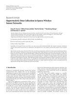
Fixing the duration of TRFR-Phase from5to30sec-
onds and increasing the number of nodes within a cluster
from 5 to 30, we obtain a branch of curves on successful
transmission rate for TRFR messages (Figure 5). Note that
TRFR’s successful transmission rate is impacted by node den-
sity (which is defined as how many nodes are there over an
area) and the length of TRFR-Phase. From experimental re-
sults, we can choose a suitable duration for TRFR-Phase to
ensure that data-gathering nodes can acquire necessary in-
formation from data-collection nodes to determine the sys-
tem schedule successfully.
3.2. Matching schedule establishment
and maintenance
According to received schedule messages (Figure 6), nodes
set up their own phase-switching schedules, which ensure
Q. Ren and Q. Liang 7
100
99
98
97
96
95

94
93
Successful transmission rate for TRFR message (%)
5 1015202530
Number of nodes in one cluster
TRFR-Phase duration
= 5 seconds
TRFR-Phase duration
= 10 seconds
TRFR-Phase duration
= 15 seconds
TRFR-Phase duration
= 20 seconds
TRFR-Phase duration
= 25 seconds
TRFR-Phase duration
= 30 seconds
Figure 5: Successful transmission rate for TRFR message.
T
(2 bits)
SRC
(8 bits)
D
TRFR
(8 bits)
D
on
(8 bits)
D
off

(8 bits)
I
r
(8 bits)
T
SRC
D
TRFR
Packet type
Source address
TRFR phase duration
D
on
D
off
I
r
On-Phase duration
Off-Phase duration
Reschedule interval
Figure 6: Schedule message packet format for A-MAC.
them to switch to the same phase simultaneously. To sim-
plify the schedule setting up process, we consider, firstly, the
scenario in which there is no clock-drift and trafficistime-
invariant.
We utilize two techniques to make our scheme robust and
feasible to use free-running timing method [8], which allows
nodes to run on their own clocks and makes contribution to
save the energy used by setting up and maintaining the global
or common timescale. Firstly, schedule messages are broad-

casted. Leveraging the property of broadcast, schedule mes-
sages can reach all data-collection nodes at the same time,
once we ignore the difference of propagation time of them
(it is reasonable since the propagation time within a clus-
ter is between 0.1 and 1 microsecond). Moreover, nodes go
to On-Phase immediately after receiving schedule messages.
Secondly, in a schedule message, all time references, such as
on-duration and off-duration, are relative values rather than
absolute values. This property can eliminate errors intro-
duced by sending time and access time. Hence, each node
within a cluster is synchronized to a reference packet (sched-
ule message) that is injected into the physical channel at the
same instant. Furthermore, after a same period of time spec-
ified by T
n
,allnodesswitchtoOff-Phase and stay there for
a T
f
period. Finally, all nodes switch back to On-Phase.A
phase is circulatedly switched like this way (see Figure 7).
Note that based on schedule messages and nodes’ local
clocks, phase-switching schedules are supposed to be estab-
lished at each node to ensure matching operations if there
is no clock-drift. Obviously, there is no global or common
timescale in our system.
As we mentioned earlier, however, mismatching opera-
tions among nodes are unavoidable, since there are always
clock-drifts caused by unstable and inaccurate frequency
standards. So it is possible that transmitters have powered on
their radios to send a message, but receivers’ radios are still

powered off. Those mismatching operations cause commu-
nication to fail. Moreover, with the accumulative clock-dr ift
becoming bigger and bigger, the impact on communications
turnstobemoreandmoreserious.
Our solution is to rebroadcast schedule message, which
forces data-collection nodes to remove accumulative clock-
drifts and to reestablish matching schedules. However, how
can data-collection nodes know the time of the next sched-
ule broadcast so as to power on their radios? The solution is
that we include reschedule interval information into sched-
ule messages. How to preestimate the value of a schedule in-
terval is another main contribution in this paper. The details
are described in Section 3.3. Flowcharts for data-gathering
nodes and data-collection nodes are modified as in Figure 8,
in which clock-drift is added and time-variant trafficiscon-
sidered.
Nevertheless, this scheme may lose efficiency in a special
situation. That is, data-collection nodes start Schedule-Phase
later than their data-gathering nodes for accumulative clock-
drifts. Consequently, the schedule broadcast will be missed
and those nodes cannot be synchronized or know the lat-
est schedule. This kind of node is named synchronization-
losing node. For this issue, we design an on-demand strat-
egy. That is, when the last On-Phase is over, synchronization-
losing nodes proactively send requests to their data-gathering
nodes. Related data-gathering nodes will reply those requests
with the latest schedule and the information on the next On-
Phase’s starting time. Then, synchronization-losing nodes
can be synchronized and reestablish their phase-switching
schedules.

3.3. Schedule interval design
The above discussions show that the matching operation
among nodes can avoid unsuccessful transmission caused
by accumulative clock-drifts. However, we also argue that it
is unnecessary to offer matching operation at all times and
for all nodes. For instance, two nodes, which have little in-
formation to exchange, need not to switch phases coinci-
dently, since their mismatching operation has little influence
on communications. Hence, some nodes could be allowed to
go out of coincidence and to be rescheduled only if necessary.
Furthermore, from (12)and(15), we note that the du-
rations of On-Phase and Off-Phase are tightly related to the
8 EURASIP Journal on Wireless Communications and Networking
Start
Collecting TRFR messages
from normal nodes
Determining the values for T
n
,
T
f
,andT
Generating schedule message
and broadcasting it locally
End
(a)
Start
Sending TRFR message
Waiting for schedule
broadcast, arrive?

N
Y
Switching to On-Phase
On-Phase is
timeout?
N
Y
Switching to Off-Phase
N
Off-Phase is
timeout?
Y
(b)
Figure 7: Without clock-drift and time-variant traffic, flowchart for (a) data-gathering nodes and (b) data-collection nodes to establish and
maintain matching schedules in A-MAC.
nodes’ traffic strength and service capability, which are het-
erogeneous for WSNs as we discussed above. Thus, besides
on-demandly removing accumulative clock-drifts and in-
forming phase-switching schedules, an additional funct ion
for schedule broadcasts is to acquire more suitable values for
essential parameters according to the system situation. This
property enables our algorithm to be an adaptive scheme in
terms of node density and traffic strength.
How to combine all factors to adjust the length of sched-
ule interval correctly is a complicated and vague task, which
impacts the p erformance in terms of energy reservation and
successful communication significantly. Since FLS is out-
standing in dealing with uncertain problems, we design a
rescheduling FLS to monitor the influence of a ccumulative
clock-drifts, the variance of traffic strength, and service ca-

pability on communications. Then we can adjust schedule
interval and power-on/off duration adaptively. We use
T
i
= ξ
i
× T
i−1
(19)
as our interval adjustment function, where T
i
is the interval
for the ith schedule broadcast, ξ
i
is the ith adjustment factor
determined by our rescheduling FLS.
In our rescheduling FLS, there are three antecedents:
(i) ratio of node with overflowing buffer (R
of
): the per-
centage of node having buffer overflowing within a
cluster;
(ii) ratio of node with high unsuccessful transmission
rate (R
hf
): the percentage of node whose unsuccessful
transmission rate is higher than a threshold within a
cluster;
(iii) ratio of node experiencing unsuccessful transmission
(R

sr
): the percentage of node having transmission fail-
ure within a cluster.
R
of
reflects traffic strength. R
hf
and R
sr
reflect the influence
of accumulative clock-drifts on communications from depth
and width aspects individually.
The consequent is the adjustment factor ( ξ
i
) for the
schedule-broadcast interval. The linguistic variables repre-
senting R
of
, R
hf
,andR
sr
are divided into three levels: low,
moderate,andhigh. ξ
i
is divided into 5 levels: highly de-
crease, decrease, unchange, increase,andhighly increase.We
use trapezoidal membership functions (MFs) to represent
low, high, highly decrease,andhighly increase, and triangle
MFs to represent moderate, decrease, unchange,andincrease.

We show those MFs in Figures 9(a) and 9(b).
The schedule interval should b e shortened when there
are many data packets missing due to accumulative clock-
drifts and/or unsuitable Off-Phase duration, otherwise the
schedule interval should be extended to reduce the energy
consumption on scheduling. Based on this fact, we design
our rescheduling FLS using rules summarized in Ta bl e 1.
For every input (R
of
, R
hf
, R
sr
), the output is defuzzified
using (20). The heights of the five fuzzy sets depicted in
Q. Ren and Q. Liang 9
Start
Collecting TRFR messages
from normal nodes
Determining the values
for T
n
, T
f
,andT
Generating schedule message
and broadcasting it locally
Next broadcast
time arrive?
N

Y
(a)
Start
Sending TRFR message
Waiting for schedule
broadcast, arrive?
N
Y
Switching to On-Phase
On-Phase is
timeout?
N
Y
N
Next broadcast
time arrive?
Y
Switching to Off-Phase
N
Off-Phase is
timeout?
Y
(b)
Figure 8: With clock-drift and time-variant traffic, flowchart for (a) data-gathering nodes and (b) data-collection nodes to establish and
maintain matching schedules in A-MAC.
1.5
1
0.5
0
012345678910

Low Moderate High
(a)
1.5
1
0.5
0
00.511.522.533.544.55
Highly decrease
Decrease Unchange Increase Highly increase
(b)
Figure 9: (a) Antecedent MFs for rescheduling-FLS and (b) consequent MFs for rescheduling-FLS.
Figure 9(b) are
¯
ξ
1
= 0.2,
¯
ξ
2
= 0.5,
¯
ξ
3
= 1.0,
¯
ξ
4
= 3.0,
¯
ξ

5
= 4.0,
y

R
of
, R
hf
, R
sr

=

15
l=1
¯
ξ
l
μ
F
l
1

R
of

μ
F
l
2


R
hf

μ
F
l
3

R
sr


15
l=1
μ
F
l
1

R
of

μ
F
l
2

R
hf


μ
F
l
3

R
sr

. (20)
The inputs of rescheduling FLS are acquired from TRFR
messages. Prior to each schedule broadcast, rescheduling
FLSs located in data-gathering nodes individually estimate
the influence degree of the accumulative clock-drift and
the change of traffic strength on communications. After
10 EURASIP Journal on Wireless Communications and Networking
TRFR-Phase
Schedule-Phase
On-Phase Off-Phase On-Phase Off-Phase
On-Phase On-Phase Off-Phase
TRFR-Phase
Schedule-Phase
On/Off Rotation 1 On/Off Rotation 2
Schedule broadcast interval
Super-time-slot 1
Super-time-slot 1
Super-time-slot i
Super-time-slot i
Figure 10: System time scheme structure for ASMAC.
Table 1: Rules for rescheduling-FLS; Ante1 is R

of
, Ante2 is R
hf
,
Ante3 is R
sr
,consequentisξ.
Rule Ante1 Ante2 Ante3 Consequent
1 Low Low Low Highly increase
2 Low Low Moderate Increase
3 Low Moderate Moderate Decrease
4 Low Moderate High Decrease
5 Moderate Low Moderate Increase
6 Moderate Low High Unchange
7 Moderate Moderate Moderate Decrease
8 Moderate Moderate High Highly decrease
9 Low High High Decrease
10 Moderate High High Highly decrease
11 High Low Moderate Increase
12 High Low High Unchange
13 High Moderate Moderate Decrease
14 High Moderate High Decrease
15 High High High Highly decrease
obtaining ξ
i
, data-gathering nodes determine the value for
the next schedule-broadcast interval according to (19). This
operation cannot only save energy through avoiding unnec-
essary schedule broadcasts and idle listening, but also ensures
an adequate data successful transmission rate.

4. ASYNCHRONOUS SCHEDULE-BASED
MAC (ASMAC) PROTOCOL
Asynchronous schedule-based MAC (ASMAC) is similar to
A-MAC. ASMAC’s system time is also divided into four
phases: TRFR-Phase, Schedule-Phase, On-Phase,andOff-
Phase (Figure 10). The same TRFR message and TRFR-Phase
duration design method are used by ASMAC. However, On-
Phase is further divided into super-time-slots, which are
composed of several normal time slots, and one source-
destination pair continuously occupies one super-time-slot.
T
(2 bits)
SRC
(8 bits)
D
off
(8 bits)
D
on
(8 bits)
SRC
1
(8 bits)
DEST
1
(8 bits)
D
df1
(8 bits)
D

s1
(8 bits)
SRC
2
(8 bits)
DEST
2
(8 bits)
D
df2
(8 bits)
D
s2
(8 bits)
SRC
i
(8 bits)
DEST
i
(8 bits)
D
dfi
(8 bits)
D
si
(8 bits)
T
SRC
D
off

D
on
D
s1
D
dfi
SRC
1
DEST
i
Packet type
Source address
Off-Phase duration
On-Phase duration
super-time-slot duration for node i
super-time-slot starts defer time
Source address for ith super-time-slot
Destination address for ith super-time-slot
Figure 11: Schedule message packet format for ASMAC.
We add ACK message as the acknowledgment for receiving
data packets successfully. A transmission is defined as an un-
successful one once the transmitter does not receive ACK af-
ter a certain period of time. The format of the schedule mes-
sage is shown in Figure 11.
Matching schedule establishment, maintenance, and
schedule interval design mechanisms of ASMAC are the same
as in A-MAC, but power-on/off duration design is somewhat
different. A new task, time-slot allocation, is added into AS-
MAC.
4.1. On-Phase/Off-Phase duration (T

n
/T
f
)design
In ASMAC, nodes perform communication in their own
super-time-slots and turn off their radios to save energy in
Off-Phase and other nodes’ super-time-slots. Hence, nodes
carry out communications orderly and contention freely.
The same criteria are utilized by ASMAC for On-Phase and
Off-Phase duration designs: trying to save more energy, keep-
ing information up to date, and avoiding losing information
due to buffer overflowing. The optimum values for T
f
and
Q. Ren and Q. Liang 11
1.5
1
0.5
0
012345678910
Low Moderate High
(a)
1.5
1
0.5
0
00.10.20.30.40.50.60.70.80.91
Ver y l ow Low Mo der ate Hig h Ver y h igh
(b)
Figure 12: (a) Antecedent MFs for allocation-FLS and (b) consequent MFs for allocation-FLS.

T
n
can be calculated:
(1) when 2W
max
< min
j

k
j
λ
j

,
T
f
=
2W
max

1+

N
l=1

μ
l
λ
l
/


1 − μ
l
λ
l

,
T
n
=
2W
max

N
l
=1

μ
l
λ
l
/

1 − μ
l
λ
l


1+


N
l=1

μ
l
λ
l
/

1 − μ
l
λ
l

;
(2) when 2W
max
≥ min
j

k
j
λ
j

,
T
f
= min

j

k
j
/λ
j
1+

N
l
=1

μ
l
λ
l
/

1 − μ
l
λ
l


,
T
n
= min
j



k
j
/λ
j


N
l=1

μ
l
λ
l
/(1 − μ
l
λ
l

1+

N
l=1

μ
l
λ
l
/


1 − μ
l
λ
l


.
(21)
4.2. Time-slot assignment
For classic TDMA systems, the system time is divided into
slots, and each user occupies cyclically repeating time slots—
abuffer-and-burst method. Thus, high-quality network syn-
chronization method is needed. Unfortunately, this premise
is troublesome for our ASMAC scheme. However, we note
that as the length of time slots increases, more transmissions
are done successfully under the same mismatching situation.
Hence, with contrast to buffer-and-burst method, we design
abuffer-and-continue method to enhance the tolerance on
accumulative clock-drifts, in which the same communication
pairs occupy sets of continuous time-slots.
In ASMAC, we design an allocation FLS to correspond-
ingly quantify transmission priorities for each node. There
are two antecedents to our allocation FLS:
(i) trafficarrivalrate(R
a
),
(ii) transmission failure rate (R
us
).
Table 2: Rules for allocation-FLS; Ante1 is the traffic arrival rate,

Ante2 is the unsuccessful transmission rate, consequent is the pri-
ority of a node performing transmission.
Rule Ante1 Ante2 Consequent
1Low Low Moderate
2LowModerateHigh
3 Low High Very hig h
4Moderate Low Low
5 Moderate Moderate Moderate
6 Moderate High High
7 High Low Very low
8HighModerate Low
9 High High Moderate
The consequent is the priority of a node performing trans-
mission (P
t
).
The linguistic variables used to represent R
a
and R
us
are
divided into three levels: low, moderate,andhigh. P
t
is di-
vided into 5 levels: very hign, high, moderate, low,andvery
low. We use trapezoidal membership functions (MFs) to rep-
resent low, high, very low,andvery high, and triangle MFs
to represent moderate, low,andhigh. We show those MFs in
Figures 12(a) and 12(b).
The transmission priority of a node should be higher

when there are more data packets waiting for transmitting
and/or its transmission failure rate is high. Based on this
fact, we design our allocation FLS using rules summarized in
Table 2. With the allocation FLS, data-gathering nodes lever-
age the information acquired from TRFR messages to quan-
tify priorities for nodes. The node owning the highest pri-
ority is the earliest one to perform communications during
On-Phase.
12 EURASIP Journal on Wireless Communications and Networking
160
140
120
100
80
60
40
Energy utilization (pk/J)
00.005 0.01 0.015 0.02 0.025 0.03 0.035
Average clock-drift rate (ms/s)
A-MAC
S-MAC
(a)
200
180
160
140
120
100
80
60

40
Energy utilization (pk/J)
00.05 0.10.15 0.20.25 0.30.35 0.40.45 0.5
Average clock-drift rate (ms/s)
ASMAC
S-MAC
TRAMA
(b)
Figure 13: Energy utilization for (a) A-MAC and (b) ASMAC.
Table 3: Physical layer parameters.
W
w min
32 W
w max
1024
MAC header 34 bytes ACK 38 bytes
CTS 38bytes RTS 44bytes
SIFS 10 μsDIFS50μs
ACK timeout 212 μs CTS timeout 348 μs
5. SIMULATION AND PERFORMANCE EVALUATION
We used the simulator OPNET to run simulations. A net-
work with 30 nodes is set up and the radio range (radius) of
each node is 30 m. Those nodes are randomly deployed in an
area of 100
× 100 m
2
and have no mobility. This network can
be treated as one cluster in a large-scale system. In order to
simplify the analysis about the impact of accumulative clock-
drifts on communications and the performance of our MAC

algorithms, we exclude the factors coming from physical layer
and network layer in our experiments. The clock-drift rate of
frequency oscillators varies from 1 to 100 microseconds every
second. Table 3 summarizes the parameters used by our sim-
ulations. The packet size is 1000 bytes. The destination for
each node’s traffic is randomly chosen f rom its neighbors.
As in [35, 36], data packets arrive according to a Poisson
process with certain rate in our simulations. Moreover, every
10 seconds, the traffic will be held for 5 seconds to simulate
bursting traffic. In our simulations, we substitute statistic av-
erage values with time-average values for data packet arrival
rate and service time.
All nodes are set with initial energy of 15 J. We use the
same energy consumption model as in [37] for radio hard-
ware. To transmit an l-symbol message for a distance d, the
radio expends:
E
Tx
(l, d) = E
Tx − elec(l)
+ T
Tx − amp(l,d)
= l × E
elec
+ l × e
fs
× d
2
;
(22)

and to receive this message, the radio expends:
E
Rx
= l × E
elec
. (23)
The electronics energy E
elec
, as described in [37], depends
on factors such as coding, modulation, pulse shaping, and
matched filtering. The amplifier energy e
fs
× d
2
depends
on the distance to the receiver and the acceptable bit er-
ror rate. In this paper, we choose E
elec
= 50 nJ/syn and
e
fs
= 10 pJ/sym/m
2
. When a node receives packets but the
destination is not for it, those packets will be discarded. T his
kind of useless receiving, that is, idle listening, uses the same
model in (23) to calculate energy consumption.
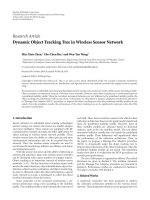
5.1. A-MAC versus S-MAC
We compared our A-MAC ag ainst S-MAC [17] without net-
work synchronization function. In our simulations, energy

utilization is assessed by the number of successfully trans-
mitted data packets per J, and the unit is pk/J. Energy uti-
lization versus clock-drift rate is plotted in Figure 13(a).Ob-
serve that A-MAC can send 17.85% to 33.33% more packets
per J. Therefore, with the same available energy and traffic
strength, the lifetime of a network will be extended about 0.2
to 0.4 times when using our algorithm A-MAC instead of S-
MAC scheme. This result demonstrates that A-MAC can im-
plement the energy reservation task successfully.
Q. Ren and Q. Liang 13
100
90
80
70
60
50
40
Successful transmission rate (%)
00.005 0.01 0.015 0.02 0.025 0.03 0.035
Average clock-drift rate (ms/s)
A-MAC
S-MAC
(a)
100
95
90
85
80
75
Successful transmission rate (%)

00.01 0.02 0.03 0.04 0.05 0.06 0.07 0.08 0.09 0.1
Clock-drift rate (ms/s)
S-MAC
TRAMA
ASMAC
(b)
Figure 14: Successful transmission rate for (a) A-MAC and (b) ASMAC.
14
12
10
8
6
4
2
Average waiting time (s)
00.005 0.01 0.015 0.02 0.025 0.03 0.035
Average clock-drift rate (ms/s)
A-MAC
S-MAC
(a)
24
22
20
18
16
14
12
10
Average waiting time (s)
00.01 0.02 0.03 0.04 0.05 0.06 0.07 0.08 0.09 0.1

Average clock-drift rate (ms/s)
ASMAC
S-MAC
TRAMA
(b)
Figure 15: Waiting time for (a) A-MAC and (b) ASMAC.
Saving energy is one of the main aims of A-MAC. How-
ever, we should not achieve this goal through sacrificing data
successful transmission rate, since communication is the ul-
timate role for communication systems. In Figure 14(a),we
plot data successful transmission rate versus clock-drift rate.
Observe that A-MAC can transmit data packets successfully
about 30.77% more than S-MAC. The reasons are, firstly,
failure transmissions are reduced because clock-drifts among
nodes are removed effectively; secondly, more energy is uti-
lized by transmitting data packets.
In Figure 15(a), we plot average waiting time versus
clock-drift rate. It is shown that A-MAC has about 33.3%
shorter waiting time than that of S-MAC. Moreover, we
set W
max
to 12 seconds for average waiting time, we found
that average waiting-time for A-MAC is always shorter than
12 seconds even at different clock-drift rates. However for
14 EURASIP Journal on Wireless Communications and Networking
100
90
80
70
60

50
40
30
20
10
0
Data successful transmission rate (%)
0 5 10 15 20 25 30 35
Tot al num ber of no d es in a c l us t er
Clock-drift rate
= 0 ms/s
Clock-drift rate
= 0.05625 ms/s
Clock-drift rate
= 0.09 ms/s
Clock-drift rate
= 0.3425 ms/s
(a)
100
90
80
70
60
50
40
30
20
10
0
Data successful transmission rate (%)

0 5 10 15 20 25 30 35
Tot al num ber of no d es in a c l us t er
Average clock-drift rate
= 0.3425 ms/s
Average clock-drift rate
= 0.225 ms/s
Average clock-drift rate
= 0.09 ms/s
Average clock-drift rate
= 0.0625 ms/s
Average clock-drift rate
= 0.05625 ms/s
Average clock-drift rate
= 0.045 ms/s
(b)
Figure 16: Network density adaptation for (a) ASMAC and (b) A-MAC.
S-MAC, the average waiting-time is longer than 12 seconds
when clock-drift rate is longer than 0.0225 ms/s. That is,
there are many out-of-date packets received when using S-
MAC. This result demonstrates our claim that our algorithm
A-MAC is a waiting-time-aware method.
5.2. ASMAC versus S-MAC and TRAMA
We compared our ASMAC against S-MAC and TRAMA [13]
without network synchronization function. Energy utiliza-
tion versus clock-drift rate is plotted in Figure 13(b).Observe
that ASMAC can send 41.176% to 56.14% more packets per
J. Therefore, with same available energy and traffic strength,
the lifetime of a network will be extended about 0.4to0.6
times when using our algorithm ASMAC instead of S-MAC
and TRAMA schemes. This result demonstrates that ASMAC

can also implement energy reservation task successfully.
In Figure 14(b), we plot data successful transmission rate
versus clock-drift rate. Observe that ASMAC can transmit
data packets successfully about 12.5% more than S-MAC,
and about 4.65% more than TRAMA.
In Figure 15(b), we plot average waiting time versus
clock-drift rate. It is shown that ASMAC has about 56.178%
shorter waiting time than TRAMA, and about 8.648% than
S-MAC. We found that the average waiting time for ASMAC
is also shorter than W
max
= 12 seconds at different clock-
drift rates. However, for TRAMA and S-MAC, the average
waiting time is longer than that threshold.
5.3. Adaptation of ASMAC and A-MAC
We investigate the influences of node density and traf-
fic strength on system performance of our algorithms. We
change node density and traffic strength individually at a set
of clock-drift situations. In Figure 16(a), we plot number of
nodes, changed from 10 to 30, in a cluster versus success-
ful transmission rate of data packet for ASMAC. Notice that
for each clock-drift rate, the vibration of successful transmis-
sion rate with the change of the node density is less than
85.714%
− 83.606% = 2.108%. The same experiment is
done for A-MAC. We can see that the vibration of success-
ful transmission rate is less than 61.96%
− 59.87% = 2.09%
(Figure 16(b)).
In Figure 17(a), we compare successful transmission rate

at different traffic arrival rates, varying from 0.1to0.5 pk/s.
This shows that for each clock-drift, the vibration of suc-
cessful transmission rate with the change of node number is
less than 97.099%
− 96.087% = 1.012% for ASMAC. The
vibration of A-MAC is less than 60%
− 58.79% = 1.21%
(Figure 17(b)).
These two experiments show that with the variance of
node density and traffic strength, network throughput can
keep almost stable through using our A-MAC and AS-
MAC protocols. The reason is that essential parameters—
reschedule interval, On-Phase,andOff-Phase durations—are
adaptively adjusted with the system situation.
Q. Ren and Q. Liang 15
100
90
80
70
60
50
40
30
20
10
0
Data successful transmission rate (%)
00.05 0.10.15 0.20.25 0.30.35 0.40.45 0.5
Traffic arrival rate (pk/s)
Clock-drift rate

= 0 ms/s
Clock-drift rate
= 0.05625 ms/s
Clock-drift rate
= 0.09 ms/s
Clock-drift rate
= 0.3425 ms/s
(a)
100
90
80
70
60
50
40
30
20
10
0
Data successful transmission rate (%)
0
0.1
15 10
Traffic arrival rate (pk/s)
Average clock-drift rate
= 0.3425 ms/s
Average clock-drift rate
= 0.225 ms/s
Average clock-drift rate
= 0.09 ms/s

Average clock-drift rate
= 0.0625 ms/s
Average clock-drift rate
= 0.05625 ms/s
Average clock-drift rate
= 0.045 ms/s
(b)
Figure 17: Traffic intensity adaptation for (a) ASMAC and (b) A-MAC.
6. CONCLUSIONS
In this paper, we proposed two energy-efficient MAC proto-
cols for WSNs: A-MAC and ASMAC. They make following
contributions compared with existing energy-efficient MAC
protocols for WSNs:
(i) saving energy at MAC layer through trading off data
waiting time and reducing energy consumption on
collision and idle listening;
(ii) utilizing free-running time scheme and schedule
broadcast to set up system schedules without establish-
ing a common timescale within a system;
(iii) exploiting a reschedule method, instead of network
synchronization, to handle mismatching operations
caused by accumulative clock-drifts;
(iv) taking advantage of fuzzy logical theories to design
rescheduling FLS and allocation FLS;
(v) proposing a traffic-strength- and network-density-
based model to optimize essential algorithm param-
eters.
Simulation results showed that not only the performance of
network is improved, but also its lifetime is extended when
A-MAC or ASMAC is used.

ACKNOWLEDGMENT
This work was supported by the US Office of Naval R e-
search (ONR) Young Investigator Program Award under
Grant N00014-03-1-0466.
REFERENCES
[1] D. Culler, D. Estrin, and M. Srivastava, “Guest Editors’ In-
troduction: overview of sensor networks,” Computer, vol. 37,
no. 8, pp. 41–49, 2004.
[2] F. Zhao and L. Guibas, Wireless Sensor Networks: An Informa-
tion Processing Approach, Morgan Kaufmann, San Francisco,
Calif, USA, 2004.
[3] M. Stemm and R. H. Katz, “Measuring and reducing energy
consumption of network modules in hand-held devices,” IE-
ICE Transactions on Communications,vol.E80-B,no.8,pp.
1125–1131, 1997.
[4] J. Chou, D. Petrovic, and K. Ramachandran, “A distributed
and adaptive signal processing approach to reducing energy
consumption in sensor networks,” in Proceedings of 22nd An-
nual Joint Conference on the IEEE Computer and Communi-
cations Societies (INFOCOM ’03), vol. 2, pp. 1054–1062, San
Francisco, Calif, USA, March-April 2003.
[5]M.L.Chebolu,V.K.Veeramachaneni,S.K.Jayaweera,and
K. R. Namuduri, “An improved adaptive signal processing ap-
proach to reduce energy consumption in sensor networks,” in
Proceedings of 38th Annual Conference on Information Science
and System (CISS ’04), Princeton, NJ, USA, March 2004.
[6] S. Balasubramanian, I. Elangovan, S. K. Jayaweera, and K.
R. Namuduri, “Distributed and collaborative tracking for
energy-constrained ad-hoc wireless sensor networks,” in Pro-
ceedings of IEEE Wireless Communications and Networking

Conference (WCNC ’04), vol. 3, pp. 1732–1737, Atlanta, Ga,
USA, March 2004.
[7] S. K. Jayaweera, “An energy-efficient virtual MIMO commu-
nications architecture based on V-BLAST processing for dis-
tributed wireless sensor networks,” in Proceedings of 1st An-
nual IEEE Communications Society Conference on Sensor and
16 EURASIP Journal on Wireless Communications and Networking
Ad Hoc Communications and Networks (SECON ’04), pp. 299–
308, Santa Clar a, Calif, USA, October 2004.
[8] J. E. Elson, “Time synchronization in wireless sensor net-
works,” Dissertation, Computer Science Department, Univer-
sity of California Los Angeles, Los Angeles, Calif, USA, 2003.
[9] C. Ma, M. Ma, and Y. Yang, “Data-centric energy efficient
scheduling for densely deployed sensor networks,” in Pro-
ceedings of IEEE International Conference on Communications,
vol. 6, pp. 3652–3656, Paris, France, June 2004.
[10] S. Singh and C. S. Raghavendra, “Pamas: power aware multi-
access protocol with signaling for ad hoc networks,” ACM SIG-
COMM Computer Communication Review, vol. 28, no. 3, pp.
5–26, 1998.
[11] P802.11, “Ieee standard for wireless lan medium access con-
trol (mac) and physical layer (phy) specifications,” November
1997.
[12] J. L. Hill and D. E. Culler, “Mica: a wireless platform for deeply
embedded networks,” IEEE Micro, vol. 22, no. 6, pp. 12–24,
2002.
[13] V. Rajendran, K. Obraczka, and J. J. Garcia-Luna-Aceves,
“Energy-efficient, collision-free medium access control for
wireless sensor networks,” in Proceedings of the 1st Interna-
tional Conference on Embedded Networked Sensor Systems (Sen-

Sys ’03), pp. 181–192, Los Angeles, Calif, USA, November
2003.
[14] L. F. W. van Hoesel, T. Nieberg, H. J. Kip, and P. J. M.
Havinga, “Advantages of a TDMA based, energy-efficient, self-
organizing MAC protocol for WSNs,” in Proceedings of IEEE
59th Vehicular Technology Conference (VTC ’04), vol. 3, pp.
1598–1602, Milan, Italy, May 2004.
[15] J. Li and G. Y. Lazarou, “A bit-map-assisted energy-efficient
MAC scheme for wireless sensor networks,” in Proceedings of
3rd International Symposium on Information Processing in Sen-
sor Networks (IPSN ’04), pp. 55–60, Berkeley, Calif, USA, April
2004.
[16] S. Biaz and Y. D. Barowski, “GANGS: an energy efficient MAC
protocol for sensor networks,” in Proceedings of the 42nd An-
nual Southeast Regional Conference (ACMSE ’04), pp. 82–87,
Huntsville, Ala, USA, April 2004.
[17] W. Ye, J. Heidemann, and D. Estrin, “An energy-efficient MAC
protocol for wireless sensor networks,” in Proceedings of 21st
Annual Joint Conference of the IEEE Computer and Communi-
cations Societies (INFOCOM ’02), vol. 3, pp. 1567–1576, New
York, NY, USA, June 2002.
[18] T. Van Dam and K. Langendoen, “An adaptive energy-efficient
MAC protocol for wireless sensor networks,” in Proceedings of
the 1st International Conference on Embedded Networked Sen-
sor Systems (SenSys ’03), pp. 171–180, Los Angeles, Calif, USA,
November 2003.
[19] J. Polastre, J. Hill, and D. Culler, “Versatile low power media
access for wireless sensor networks,” in Proceedings of the 2nd
International Conference on Embedded Networked Sensor Sys-
tems (SenSys ’04), pp. 95–107, Baltimore, Md, USA, November

2004.
[20] S. Jayashree, B. S. Manoj, and C. S. R. Murthy, “On using bat-
tery state for medium access control in ad hoc wireless net-
works,” in Proceedings of the 10th Annual International Confer-
ence on Mobile Computing and Networking (MobiCom ’04),pp.
360–373, Philadelphia, Pa, USA, September-October 2004.
[21] E S.JungandN.H.Vaidya,“ApowercontrolMACprotocol
for ad hoc networks,” in Proceedings of the 8th Annual Interna-
tional Conference on Mobile Computing and Networking (Mo-
biCom ’02), pp. 36–47, Atlanta, Ga, USA, September 2002.
[22] S. Bregni, Synchronization of Digital Telecommunications Net-
works , John Wiley & Sons, New York, NY, USA, 2002.
[23] F. Cristian, “Probabilistic clock synchronization,”
Distributed
Computing, vol. 3, no. 3, pp. 146–158, 1989.
[24] R. Gusella and S. Zatti, “The accuracy of the clock synchro-
nization achieved by TEMPO in Berkeley UNIX 4.3 BSD,”
IEEE Transactions on Software Enginee ring,vol.15,no.7,pp.
847–853, 1989.
[25] T. K. Srikanth and S. K. Toueg, “Optimal clock synchroniza-
tion,” Journal of the ACM, vol. 34, no. 3, pp. 626–645, 1987.
[26] W. Su and I. F. Akyildiz, “Time-diffusion synchronization pro-
tocol for wireless sensor networks,” IEEE/ACM Transactions on
Networking, vol. 13, no. 2, pp. 384–397, 2005.
[27] J. M. Mendel, “Fuzzy logic systems for engineering: a tutorial,”
Proceedings of the IEEE, vol. 83, no. 3, pp. 345–377, 1995.
[28] E. H. Mamdani, “Application of fuzzy logic to approximate
reasoning using linguistic synthesis,” IEEE Transactions on
Computers, vol. 26, no. 12, pp. 1182–1191, 1977.
[29] J. M. Mendel, Uncertain Rule-Based Fuzzy Logic Systems: Intro-

duction and New Directions, Prentice-Hall, Upper Saddle River,
NJ, USA, 2001.
[30] C. V. Altrock, “Fuzzy logic design: methodology, standards,
and tools,” Electronic Engineering Times, July 1996.
[31] L. H. Bao and J. J. Garcia-Luna-Aceves, “Hybrid channel access
scheduling in ad hoc networks,” in Proceedings of 10th IEEE
International Conference on Network Protocols (ICNP ’02),pp.
46–57, Paris, France, November 2002.
[32] D. Bertsekas and R. Gallager, Data Networks, Prentice-Hall,
Upper Saddle River, NJ, USA, 1987.
[33] M. M. Carvalho and J. J. Garcia-Luna-Aceves, “Delay anal-
ysis of IEEE 802.11 in single-hop networks,” in Proceedings
of 11th IEEE International Conference on Network Protocols
(ICNP ’03), pp. 146–155, Atlanta, Ga, USA, November 2003.
[34] G. Bianchi, “Performance analysis of the IEEE 802.11 dis-
tributed coordination function,” IEEE Journal on Selected Ar-
eas in Communications, vol. 18, no. 3, pp. 535–547, 2000.
[35] A. Manjeshwar, Q A. Zeng, and D. P. Agrawal, “An analytical
model for information retrieval in wireless sensor networks
using enhanced APTEEN protocol,” IEEE Transactions on Par-
allel and Distributed Systems, vol. 13, no. 12, pp. 1290–1302,
2002.
[36] V. P. Mhatre, C. Rosenberg, D. Kofman, R. Mazumdar, and N.
Shroff, “A minimum cost heterogeneous sensor network with
a lifetime constraint,” IEEE Transactions on Mobile Computing,
vol. 4, no. 1, pp. 4–14, 2005.
[37] W. B. Heinzelman, A. P. Chandrakasan, and H. Balakrishnan,
“An application-specific protocol architecture for wireless mi-
crosensor networks,” IEEE Transactions on Wireless Communi-
cations, vol. 1, no. 4, pp. 660–670, 2002.

Qingchun Ren received her B.S. and M.S.
degrees from University of Electrical Sci-
ence and Technology of China, in 1997 and
2003, respectively, both in electrical engi-
neering. She is working towards the Ph.D.
degree in electrical engineering at The Uni-
versity of Texas at Arlington. Prior to that,
she was a Member of the technical staff
at WATT Electronic Co., Ltd. at Shenzhen,
China. Since August 2003, she has been
a Research Assistant in the Wireless Communication Network
Group, The University of Texas at Arlington. Her research interests
Q. Ren and Q. Liang 17
are in sensor networks (energy efficiency, cross-layer design, opti-
mal sensor deployment, etc.), fuzzy logic systems, and query pro-
cessing for sensor database systems.
Qilian Liang received the B.S. degree from
Wuhan University, China, in 1993, the M.S.
degree from Beijing University of Posts and
Telecommunications in 1996, and the Ph.D.
degree from University of Southern Califor-
nia (USC) in May 2000, all in electrical en-
gineering. He joined the faculty of The Uni-
versity of Texas at Arlington in August 2002.
Prior to that, he was a Member of the tech-
nical staff in Hughes Network Systems Inc.
at San Diego, California. His research interests include sensor net-
works (energy efficiency, cross-layer design, optimal sensor deploy-
ment, etc.), wireless communications, wireless networks, commu-
nication theory, signal processing for communications, fuzzy logic

systems and applications, multimedia network traffic modeling and
classification, collaborative and distributed sig nal processing. He
has published more than 90 journal and conference papers, 4 book
chapters, and has 6 US patents pending. He received 2002 IEEE
Transactions on Fuzzy Systems Outstanding Paper Award, 2003
US Office of Naval Research (ONR) Young Investigator Award,
and 2005 UTA College of Engineering Outstanding Young Faculty
Award.