Báo cáo hóa học: " Research Article An Analysis Framework for Mobility Metrics in Mobile Ad Hoc Networks" ppt

Hindawi Publishing Corporation
EURASIP Journal on Wireless Communications and Networking
Volume 2007, Article ID 19249, 16 pages
doi:10.1155/2007/19249
Research Article
An Analysis Framework for Mobility Metrics in
Mobile Ad Hoc Networks
Sanlin Xu, Kim L. Blackmore, and Haley M. Jones
Department of Engineering, Faculty of Engineering and Information Technology, Australian National University,
ACT 0200, Australia
Received 31 January 2006; Revised 9 October 2006; Accepted 9 October 2006
Recommended by Hamid Sadjadpour
Mobile ad hoc networks (MANETs) have inherently dynamic topologies. Under these difficult circumstances, it is essential to have
some dependable way of determining the reliability of communication paths. Mobility metrics are well suited to this purpose. Sev-
eral mobility metrics have been proposed in the literature, including link persistence, link duration, link availability, link residual
time, and their path equivalents. However, no method has been provided for their exact calculation. Instead, only statistical ap-
proximations have been given. In this paper, exact expressions are derived for each of the aforementioned metrics, applicable to
both links and paths. We further show relationships between the different metrics, where they exist. Such exact expressions con-
stitute precise mathematical relationships between network connectivit y and node mobility. These expressions can, therefore, be
employed in a number of ways to improve performance of MANETs such as in the development of efficient algorithms for routing,
in route caching, proactive routing, and clustering schemes.
Copyright © 2007 Sanlin Xu et al. This is an open access article distributed under the Creative Commons Attribution License,
which permits unrestricted use, distribution, and reproduction in any medium, provided the original work is properly cited.
1. INTRODUCTION
Mobile ad hoc networks (MANETs) are comprised of mobile
nodes communicating via (potentially multihop) wireless
links. Mobility of the nodes causes communication links to
be dynamic, affecting path reliability. Frequent path break-
age, requiring discovery of new routes, leads to excessive
end-to-end delay and affects the quality of service for delay-
sensitive applications.

Understanding node mobility is one of the keys to deter-
mine the potential capacity of an ad hoc network. Various
mobility metrics have been proposed as measures of topo-
logical change in networks. Metrics describing the link or
path stability allow adaptive routing in MANETs based on
predicted link behavior. A range of routing protocols based
on predictive mobility metrics has been shown to increase
the packet delivery ratio and to reduce routing overhead
[1–6].
We consider a range of mobility metrics: link (path)
availability, link (path) persistence, link (path) residual time,
and link (path) duration. Many of these metrics have been
considered previously, (see [1–3, 7–13]), although the nam-
ing has not been consistent. We seek to identify the relation-
ships between the various metrics and provide a consistent
nomenclature. In particular, there is considerable confusion
in the literature about the term “link availability.” The term
is generally used to describe the probability that a currently
active link wil l be active at a particular time in the future.
However, some authors require that the link should exist for
the whole of the intervening period, while others do not. The
probability of existence will be considerably increased in the
latter case.
To alleviate this confusion, we introduce the new terms
link persistence and path persistence to describe the contin-
uous link and path availabilities, and reserve the term link
(path) availability to describe the noncontinuous case [14].
That is, the link (path) persistence is the probability that a
link (path) continuously lasts until a future time k given that
it existed at time 0. In the perspe ctive of link persistence, once

the link is broken, it no longer exists.
We present a theoretical analysis framework for calculat-
ing the eight mobility metrics presented, for nodes moving
according to a given synthetic mobility model. Our frame-
work can be applied to any mobility model that admits a
Markov process describing node separation. This theoretical
approach is in contrast to most research to date w h ich has
been based on simulation results and empirical analysis of
mobility metrics.
2 EURASIP Journal on Wireless Communications and Networking
Many random mobility models have been proposed [15],
however, as yet, statistical analysis of the induced network
connectivity is generally unavailable. One of the few which
can be described by simple probability distribution functions
is the random-walk mobility model (RWMM), which we use
to illustrate the use of our framework. (Future work will in-
volve the statistical description of more realistic models, sim-
ilar to [16], and application of our framework to them.)
The calculated metrics can be useful as an aid to predict-
ing link reliability for routing purposes [5, 17]. Moreover,
random mobility models are regularly used for protocol eval-
uation, so our work is important to facilitate comparison of
the evaluation environment with practical implementation
environments.
The main contributions of this paper are (1) introduc-
tion of notion of link (path) persistence and its calculation
method, (2) expressions for the expected link (path) dura-
tion and its PDF, (3) expressions for the expected link (path)
residual time and its PDF which are der ived using a random
mobility model rather than a nonrandom travelling pattern

(straight-line mobility model), (4) an exact expression for
link (path) availability which matches the simulation data
well for any given time interval.
We begin with definitions in Section 2 for the mobility
metrics we investigate, with a discussion of related work in
the literature. In Section 3 we develop two Markov chain
models of the evolution of the separation distance between
two nodes. In Section 4 the Markov chain models are used
to develop exact expressions for the aforementioned mobil-
ity metrics. In Section 5 we apply the framework developed
in the previous two sections to the random walk mobility
model. In Section 6 we compare our theoretical results for
the RWMM with simulation results. Finally, we present con-
clusions and further work in Section 7.
2. MOBILITY METRIC TAXONOMY
We define a series of mobility measures for links and for
paths. As explained in the introduction, most of these have
appeared in the literature, sometimes under different names,
but they have not previously been gathered together as we
have done here.
The following definitions do not make any assumptions
about what it means for a link to exist, but do assume that it
is possible to determine at any point in time whether or not
a link does exist. Links are understood to be “on” or “off”at
any point in time, as it is common in the existing literature
on mobility in MANETs. In reality, fading links are the norm
in wireless communication networks at the scales relevant
for ad hoc networks [9]. In such cases, link availability is an
appropriate metric to employ. However, schemes which use
network topology information are sensitive to the length of

time for which a link is consistently “on.” Therefore, our re-
maining metrics—persistence, residual time, and duration—
assume that the link is “on,” and consider how long it wil l
continue to be “on.”
An h hop path between two nodes consists of a chain of
h
− 1 intermediate nodes connecting them. Each node in the
chain has an active link with the nodes either side of it in the
chain, effectively forming a transmission path between the
two nodes of interest. A link could be described as a 1-hop
path. We define each of the metrics for paths, and define the
corresponding link metrics as special cases for which h
= 1.
The first two metrics, path (link) availability and persis-
tence, are probabilities—they correspond to the probability
that a path (link) exists at a certain time in the future given
that it exists now. One can see intuitively that in most situ-
ations, this probability decreases as the wait time increases.
The difference between availability and persistence lies in the
requirement that the path (link) may disappear and reappear
during the wait time in the case of availability, but may not
do so in the case of persistence.
The remaining metrics are measured in units of time—
referring to the length of time that a path (link) exists. Resid-
ual time can be measured from any point in the life of the
path (link), whereas path (link) duration is measured from
the time the path (link) is first “on” until the time the path
(link) is next “off.” In the case where nodes move accord-
ing to a synthetic mobility model, the residual time and du-
ration are random variables. We calculate their probability

mass functions (PMFs) and expected values in Section 4.
(i) Path availability A(t, h)
Givenanactivepathwithh hops between two nodes at time
0, the path availability [5]attimet is defined as the prob-
ability that the path exists at time t, given that it existed at
time,
A(t, h)  Pr

available at time t | available at time 0

.
(1)
The path may have been broken, possibly several times, be-
tween time 0 and time t.Thelink availability is denoted by
A(t)  A(t,1).
Path and link availability were proposed by McDonald
and Znati [5].
(ii) Path persistence P (t, h)
Givenanactivepathwithh hops between two nodes at time
0, the path persistence, as a function of time, is defined as the
probability that the path will continuously last until at least
time t, given that it existed at time 0,
P (t, h)  Pr

last until at leas time t | available at time 0

.
(2)
That is, P (t, h) is the probability that the path is continu-
ously in existence from time 0 until at least time t.Thelink

persistence is denoted by P (t)  P (t,1).
Link persistence is called “link availability” in [18, 19].
(iii) Path residual time R(h)
Given an active path with h hops between two nodes at time 0
(which may also have been active for some time immediately
prior to time 0), the path residual time, R(h), is the length
Sanlin Xu et al. 3
of time for which the path will continue to exist until it is
broken. The link residual time is denoted by R  R(1).
Link residual time has been referred to as the “link’s
residual lifetime” [8], “link available time” [13], “link expi-
ration time” [2], and “expected link lifetime” [3]. Path resid-
ual time has been referred to as “path’s residual lifetime”
[8], “available time in multihop” [13], and “route expiration
time” [2].
(iv) Path duration D(h)
Given that a path becomes active at time 0, the path duration
[12] D (h) is the length of time for which the path w ill con-
tinue to exist until it is broken. That is, the path duration is
the path residual time from the instant the path first becomes
available, and it is a measure of stability of the path between
a pair of nodes. It could be understood as a maximal value
of the path residual time. The link duration [1]isdenotedby
D  D (1).
We can divide these metrics into two groups based on
whether a persistent connection is required (persistence,
residual time, and duration) or an intermittent connection
is acceptable (availability).
2.1. Related work
Each of the metrics have been studied in var ious ways by var-

ious authors. Here we give a brief overview.
In [5, 11], path availability is used to divide mobile nodes
into clusters. The link availability and path availability were
theoretically analyzed, for nodes moving according to a vari-
ant of the random-walk mobility model. However they em-
ploy a Rayleigh approximation for relative movement be-
tween a pair of mobile nodes (MNs), which does not work
well when taken over short time intervals, particularly for
the path availability calculation. By contrast, the calculation
method presented in this paper is accurate for any time in-
terval.
Link persistence is calculated approximately by Qin [19]
for nodes moving according to the random-walk mobility
model (though they call it link availability). In [13]anex-
pression for link persistence is derived for a simple straight-
line mobility model. A mobility metric that is similar to
link persistence is determined in [6, 10] using a combina-
tion of calculation and experimental evaluation, for modified
random-walk and random waypoint mobility models.
Link (path) residual time is widely used in proactive rout-
ing schemes. The mechanism is that when a communicating
path is active between two MNs, the destination node can es-
timate the link (path) residual time by means of a prediction
algorithm. New route discovery is initiated early by detect-
ing that an active link is likely to be broken and an alterna-
tive route is built before link failure. In many cases, this is
achieved by assuming that the MNs do not change movement
direction when communicating with each other [2, 3, 13]
(a straight-line mobility model), which is clearly quite a re-
strictive assumption. Link residual time is evaluated by sim-

ulation in [8], for nodes moving according to a variety of
synthetic mobility models.
The concept of link duration was introduced by Boleng
et al. [1] as a mobility metric to enable adaptive routing.
Link duration is a good indicator of protocol performance
measures such as data packet delivery ratio and end-to-end
delay. Furthermore, it is computable in real network imple-
mentations without global network knowledge. Bai et al. [7]
and Sadagopan et al. [12], investigate link duration and path
duration experimentally, for four different mobility models
corresponding to routing protocols such as AODV and DSR,
based on simulations. Han et al. [20] give an approximate
calculation for link duration and path duration for a r an-
dom waypoint mobility model. In this paper, we determine
an exact expression for the PMF of node separation distance
when a link is set up and conclude that link (path) duration
is a special case of link (path) residual time.
2.2. Metric calculation
In general, each of the above mobility metrics will differ be-
tween particular links (paths). If the objective is to predict
future connectivity of a particular link (path), specific infor-
mation about the link (path) must be known—whether mea-
sured [18] or assumed [5]. If, on the other hand, the objective
is to characterize the degree of mobility of the network a s a
whole, it is necessary to average over all possible links (paths)
[1].
Our framework al lows calculation of the mobility met-
rics under some random mobilit y model. In this case, link
residual time and link duration are random variables. Con-
sequently, the network average link residual time and link

duration are also random variables. Thus, we consider the
expected value of the network average for these entities.
Mobility models employed in simulation-based perfor-
mance evaluation usually assume that all nodes move in an
i.i.d. random manner. In this case, the expected value of the
mobility metric associated with individual links (or paths)
will be identical, and equal to the network average. Such
assumptions may also provide useful predictions of future
connectivity when no aprioriknowledge of individual node
characteristics exists.
We will employ the notation
A(k, h), P (k, h), R(h)to
denote the network average values of availability, persistence,
and residual time (omitting the argument h
= 1 when links,
rather than paths, are of interest). Under our assumptions,
the link duration D and path duration D(h) do not need
to be augmented in this manner as the expected value of the
network average is identical to the expected value for an in-
dividual link (or path).
In our calculations, the link-based mobility metrics, ex-
cept link duration, depend (only) on the initial separation
of nodes. The path-based mobility metrics, except path du-
ration, depend (only) on the initial separation along all
hops in the path. Therefore, we augment the notation for
availability, p ersistence, and residual time to include L
0
,
the separa tion distance at time 0. The link-based mobility
metrics become A(k; L

0
), P (k; L
0
), and R(L
0
). The path-
based mobility metrics become A(k, h; L
0
(1), , L
0
(h)),
P (k, h; L
0
(1), , L
0
(h)), and R(h; L
0
(1), , L
0
(h)), where
4 EURASIP Journal on Wireless Communications and Networking
L
0
(i) is the initial separation of the nodes constituting the
ith hop in a particular path.
Having established definitions for each of the mobility
metrics of interest, we next develop generic expressions for
each of the mobilit y metrics, using a Markov chain model.
(Using a Markov chain model allows for random mobility
models for which no closed-form expression may be found

for the PDF of the mobility, which is most often the case.)
These expressions may then be applied to any particular ran-
dom mobility model by substituting in the appropriate PDF.
The random-walk mobility model is used as an example in
Section 5.
3. MARKOV CHAIN DESCRIPTION OF
NODE SEPARATION DISTANCE
AMarkovchainmodel(MCM)givesamodelfortheevo-
lution of the random process it is describing. We u se an
MCM to describe the evolution of the separation distance
between nodes in an ad hoc network, moving according to a
memoryless random mobility model. We will use the MCM
to derive mathematical expressions for each of the mobility
metrics introduced in Section 2.
In order to apply Markov chain methods, we examine
node separation after periods of fixed time length, termed
epochs. We assume that the duration of the epochs and the
speed of the nodes are such that the path persistence after
one epoch, P (1, h), is approximately one, and the path resid-
ual time, R(h), is considerably more than one epoch. In this
case, there is no significant error introduced by discretizing
the time via epochs.
3.1. Notation for model development
The status of a wireless link depends on numerous system
and environmental factors that affect transmitter and re-
ceiver’s transmission range. A widely applied, albeit opti-
mistic, model is used in this paper, whereby transmission
range is approximated by a circle of radius r corresponding
to a signal strength threshold. Thus, if the separation distance
between a pair of nodes of interest is less than r,itisassumed

that the link between them is active.
All of the mobility metrics are based on the probability
of a pair of nodes going out of range. That is, we are inter-
ested in the behavior of the separation distance between a
pair of nodes. An MCM can be employed to calculate the mo-
bility metrics in Section 2 if the separation distance between
two nodes is a Markov process. Assume that the movement
of nodes in the network can be described by i.i.d. random
processes. Let the random variable representing the separa-
tion distance between two nodes at epoch m be L
m
, and let
l
m
denote an instance of L
m
.
1
We assume that the PDF of the
L
m+1
is dependent only on L
m
. Then separation distance is a
Markov process and the transition probabilities for the MCM
1
Throughout this paper, we use the convention of capital letters for ran-
dom variables and the corresponding lowercased letters for instances of
random variables.
0 r

Separation
distance
e
1
e
i
ε
e
n
e
n+1
e
n+ j
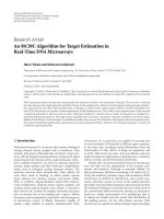
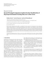
Figure 1: Depiction of state space for distance between a pair of
nodes in the intermittent metric group, where communication links
for nodes which move outside the transmission range, and back in
again, are considered to be the “same” link.
are derived from f
L
m+1
|L
m
(l
m+1
| l
m
). This PDF is determined
by the mobility model being used.
3.2. State-space derivation
We divide the node separation distance from 0 to r into n

bins of width ε. If a link exists, the node separation at epoch
m, L
m
, falls into one of these bins. If we label state i, e
i
, then
the state space of the distance between the two nodes is E
=
{
e
1
, , e
i
, }. T he state space for distances greater than r
differs for the two mobility metric groups. We examine each
group separately below.
3.2.1. State space for intermittent metric group
In this case the state space for distances greater than r consists
of an infinite number of states, each corresponding to a bin
of width ε,asillustratedinFigure 1. The node separation L
m
is in e
i
if L
m
= l
m
,where
(i
− 1)ε ≤ l

m
<iε, i ∈ Z
+
. (3)
3.2.2. State space for persistent metric group
The state space for metrics in the persistent group requires an
absorbing state which, once reached, cannot be escaped. The
absorbing state represents any distance greater than the com-
munication range r. If the distance between the two nodes
reaches the absorbing state, the communication link is con-
sidered to be broken. If the nodes move back within commu-
nication range, a new link is considered to have been formed.
In this model, the state of the node separation distance,
L
m
= l
m
,isgovernedby
(i
− 1)ε ≤ l
m
<iε, i ∈ [1, , n],
l
m
>r, i = n +1.
(4)
3.3. Initial probability vector
The Markov chain process is an evolving process. The proba-
bility of being in any particular state changes with time. Thus,
we begin with an initial probability vector which denotes the

probability of the initial node separation distance, L
0
= l
0
,
being in each of the states at epoch 0. The initial probability
vector P(0) can be written as
P(0)
=

p
1
(0) p
2
(0) ··· p
n
(0) ···

,(5)
Sanlin Xu et al. 5
where
p
i
(0) = Pr

l
0
∈ e
i


⎧
⎪
⎨
⎪
⎩
1 ≤ i ≤ n + 1 for persistent links,
i
∈ Z
+
for intermittent links.
(6)
Further, as the links are assumed to be active at epoch 0, that
is, in a state with index at most n,

n
i
=1
p
i
(0) = 1.
ThechoiceofP(0) differs according to whether the ob-
jective is to determine the mobility metric for a particular
link, or the network average for the metric. In the first case,
the initial separation distance, l
0
<r, for the link is known,
and the initial state, e
i
, is determined according to (3)or(4),
where m

= 0andi ∈ [1, , n]. Then, the initial probability
vector , denoted by P
L
0
(0), has only one nonzero element:
p
i
(0) =
⎧
⎪
⎨
⎪
⎩
1ifl
0
∈ e
i
,
0 otherwise.
(7)
For network average mobility metrics, it is necessary to de-
termine how the mobile node positions distributed in a t wo-
dimensional space. If the nodes are uniformly distributed
over the network area (as it is the case for nodes moving ac-
cording to a r andom walk in a bounded region), the distribu-
tion of all separation distances is approximately Rayleigh (it
is not exact if the network area is bounded). If, in addition,
the transmission range is much s maller than the network
area, then we can approximate the distribution of node sepa-
ration distances in the range 0 to r as being linear, as follows:

f
L
0

l
0

=
⎧
⎪
⎨
⎪
⎩
2l
0
r
2
,0≤ l
0
≤ r,
0, l
0
>r.
(8)
Thus, for network average metrics, when nodes are uni-
formly distributed, the initial condition vector, denoted
P
net
(0), has elements
p

i
(0) =
⎧
⎪
⎨
⎪
⎩
(2i − 1)
ε
2
r
2
,0≤ i ≤ n,
0, i>n.
(9)
To reiterate, this value of P
net
(0)isonlyappropriatefor
networks with uniformly distributed nodes. For many inter-
esting mobility models, nodes are not unifor mly distributed
[21].
A third initial condition vector, P
new
(0), will be intro-
duced in Section 4.1.4 to describe the PDF of node separa-
tion for links when they first become active.
3.4. Probability transition matrix
Having established the form of the initial condition vector
for the different contexts, we now introduce the probability
transmission matrices for the two metric groups.

3.4.1. Intermittent metric group transition matrix
Let the separation distance l
m
between two nodes be in state
e
i
. After one epoch, the separation distance l
m+1
must be in
the range

max

0, l
m
− 2v
max

, l
m
+2v
max

, (10)
where v
max
is the maximum speed that can be attained by the
nodes. This corresponds to l
m+1
being in e

j
such that
j
∈

max(1, i − γ), i + γ

, γ :=

2v
max
ε

, (11)
where γ is the maximum number of states that can be crossed
in a single epoch. When there is no absorbing state, as de-
picted in Figure 1, the transition matrix is denoted by the
infinite-size mat rix A
int
,where
A
int
=
⎡
⎢
⎢
⎢
⎢
⎢
⎣

a
1,1
··· a
1,n
···
.
.
.
.
.
.
.
.
.
a
n,1
··· a
n,n
···
.
.
.
.
.
.
.
.
.
⎤
⎥

⎥
⎥
⎥
⎥
⎦
, (12)
and a
i, j
is the probability of transition from e
i
to e
j
in a given
epoch. We note that for all i, j, a
i, j
≥ 0and

j
a
i, j
= 1(i.e.,
node i must move somewhere).
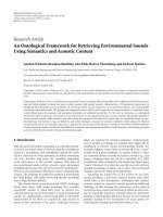
To calculate the transition probabilities between any two
states in the nonabsorbing state model, as illustrated in
Figure 2, consider the state space for the nonabsorbing state
model at epoch m. The transition probabilities are given by
a
i, j
= Pr


e
i
−→ e
j

=
Pr

l
m+1
∈ e
j
| l
m
∈ e
i

=

jε
( j
−1)ε

iε
(i
−1)ε
f
L
m+1
|L

m

l
m+1
| l
m

f
L
m

l
m

dl
m
dl
m+1
,
(13)
where the conditional PDF f
L
m+1
|L
m
(l
m+1
| l
m
)isdependent

upon the particular mobility model. Now, the PDF f
L
m
(l
m
)
varies with time m.However,ifε is sufficiently small,wecan
assume that independently of m, L
m
is approximately uni-
formly distributed within the ith bin. In this case,
f
L
m

l
m

≈
1
ε
. (14)
Moreover, we can approximate the PDF of the conditioned
separation distance from any point in e
i
to any point in e
j
by
the value of the PDF at the midpoint of the two states, such
that

f
L
m+1
|L
m

l
m+1
∈e
j
|l
m
∈e
i

≈
f
L
m+1
|L
m

j −
1
2

ε |

i −
1

2

ε

.
(15)
Thus, we have
a
i, j
≈ εf
L
m+1
|L
m

j −
1
2

ε |

i −
1
2

ε

, (16)
giving us an expression which closely approximates the tran-
sition probabilities, as long as we choose the state widths

small enough.
6 EURASIP Journal on Wireless Communications and Networking
0(i γ 1) εl
m
iε ( j 1)εjε (i + γ) ε
Separation
distance
e
1
e
2
ε
e
i γ
e
i
e
j
e
i+γ
e
n
e
n+1
a
i,i γ
a
i,i
a
i,j

a
i,i+γ
f
L
m+1
L
m

l
m+1
l
m

Figure 2: Depiction of state space for the nonabsorbing state model, showing the state transition probabilities, a
i,j
, the probability of trans-
ferring from e
i
to e
j
after one epoch, for a given state i and various states j.
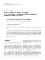
0 r
Separation
distance
e
1
e
i
ε
e

n
e
n+1
Absorbing
state
Figure 3: State space for distance between a pair of nodes in the
persistent metric group, where separations greater than the trans-
mission range (absorbing state) result in a link being discarded.
3.4.2. Persistent metric group transition matrix
Recalling that for the persistent metric group, there are n +1
possible states, as shown in Figure 3, we let the (n+1)
×(n+1)
state transition matrix, with absorbing state, be denoted by
A
pst
,where
A
pst
=
⎡
⎢
⎢
⎢
⎢
⎣
a
1,1
··· a
1,n
a

1,n+1
.
.
.
.
.
.
.
.
.
.
.
.
a
n,1
··· a
n,n
a
n,n+1
0 ··· 01
⎤
⎥
⎥
⎥
⎥
⎦
. (17)
The entries indicating the probabilities of entering the ab-
sorbing state, that is, the rightmost column of A
pst

,aregiven
by
a
i,n+1
= 1 −
n

j=1
a
i, j
. (18)
The last row of A
pst
indicates the probability of transition
from the absorbing state.
The probabilities of moving between each pair of nonab-
sorbing states are given by the upper left block of A
pst
:
Q
=
⎡
⎢
⎢
⎣
a
1,1
··· a
1,n
.

.
.
.
.
.
.
.
.
a
n,1
a
n,n
⎤
⎥
⎥
⎦
, (19)
where entr y a
i, j
is given by (16).
3.5. Separation probability vector after k epochs
Using the transition matrices defined in Section 3.4, and the
initial probability vectors defined in Section 3.3,wecancal-
culate the probability vector of the separation distance after k
epochs P(k). For the intermittent metr ics, where there is no
absorbing state,
P(k)
= P(0)A
k
int

, (20)
where P(k) is an infinite-length vector with elements p
i
(k),
describing the probability that the separation distance L
k
is
in e
i
attheendofepochk and A
int
is from (12).
Similarly, for the persistent metrics, where the separation
distance state space does include an absorbing state, P(k)is
an (n +1)-vector
P(k)
= P(0)A
k
pst
, (21)
where A
pst
is from (17).
In either case, necessarily,

i
p
i
(k) = 1, (22)
where i ranges from 1 to n + 1 if there is an absorbing state,

and from 1 to
∞ if there is no absorbing state.
In summary, P(k) gives the discrete probability distribu-
tion of the separation distance between a pair of nodes after
k epochs. It is discrete, but may be made as incremental as
desired by appropriately choosing ε, the width of each state.
4. MOBILITY METRIC CALCULATIONS
We have presented expressions for the discrete probability
distribution of the separation distance between a pair of
nodes at any time in (20)and(21). We now use these to de-
rive expressions for each of the mobility metrics defined in
Section 2. Because the Markov chain development requires
discrete-time intervals, in our mobility metric calculations,
we consider discrete-time versions of the metrics, replacing
time t with epoch k.
Sanlin Xu et al. 7
4.1. Expressions for link-based metrics
Calculation of the link-based metrics is achieved via di-
rect application of Markov chain methods, using the ini-
tial probability vectors and transition matrices introduced in
Section 3.
4.1.1. Link availability A(k)
Link availability is an intermittent mobility metric—the link
maybebrokenatsometimebeforeepochk,butmustbe
reestablished by epoch k. Thus we use the probability tran-
sition matrix with no absorbing state A
int
. The probability
of the link being in existence after k epochs is the sum of
the probabilities of L

k
being in one of e
1
to e
n
at epoch k.
Thus, the link availability is the sum of the first n elements
of P(k)in(20). The general equation for link availability is,
therefore,
A(k)
=
n

i=1
p
i
(k), (23)
where p
i
(k) are the elements of P(k) = P(0)A
k
int
.
The link availability for a particular initial separation
A(k; L
0
) uses the initial condition vector P
L
0
(0) with ele-

ments defined in (7). The network average link availability
A(k) uses the initial probability vector P
net
(0) from (9).
4.1.2. Link persistence P (k)
Link persistence is determined in the same way as link avail-
ability, with the exception that the transition matrix with ab-
sorbing state A
pst
is used. Thus, the general equation for link
persistence is
P (k)
=
n

i=1
p
i
(k) = 1 − p
n+1
(k), (24)
where p
n+1
(k) is the final element of the vector P(k) =
P(0)A
k
pst
.
The link persistence for a particular initial separation,
P (k; L

0
) uses the initial condition vector P(0) = P
L
0
(0) with
elements defined in (7). The network average link persistence
P (k) uses the initial condition vector P
net
(0) from (9).
4.1.3. Link residual time R
The probability that the link residual time is, at most, k
is equal to the probability that after epoch k, the separa-
tion distance is in the absorbing state e
n+1
.Wecanwritethe
(discrete) cumulative density function (CDF), F
R
(k), of the
link residual time, as
F
R
(k) = Pr{R ≤ k}=p
n+1
(k), (25)
where p
n+1
(k)isdefinedinSection 4.1.2. Therefore, the
probability m ass function (PMF), f
R
(k), of the link residual

time is
f
R
(k) = Pr{R = k}=p
n+1
(k) − p
n+1
(k − 1). (26)
In Section 6 we illustrate that this PMF is approximately ex-
ponential.
The expected value of the link residual time can then be
written as
E
{R}=
∞

k=1
kf
R
(k) =
∞

k=1
k

p
n+1
(k) − p
n+1
(k − 1)


.
(27)
This holds for both link-specific residual t ime R(L
0
)and
network average residual time
R by again using the appro-
priate initial condition vector. Due to the exponential decay
of the PMF, terms in this sum are negligible for large k,mean-
ing that truncation at an appropriate point will result in neg-
ligible error, allowing feasibility of calculation.
Alternatively, the link residual time can be determined
directly from the fundamental matrix, F [22],
F
=

I
n
− Q

−1
, (28)
where I
n
is the n×n identity matrix, and Q is defined in (19).
The sum of the elements of the ith row of F is the expected
link residual time for links starting in e
i
,

E

R

L
0

=
n

j=1
F
i, j
, L
0
= l
0
∈ e
i
. (29)
The expected value of the network average link residual time
is
E
{R}=
n

i=1
p
i
(0)

n

j=1
F
i, j
, (30)
where p
i
(0) are elements of P
net
(0) from (9).
4.1.4. Link duration D
Link duration is effectively a special case of the link residual
time, with the requirement that L
0
= r. That is, the link du-
ration is the link residual time at the time of formation of the
link—how long the link lasts from beginning to end. In fact,
as the mobility model is discrete in time, L
0
∈ [r − 2v
max
, r),
since we only examine the connectivity at the end of each
epoch. Therefore, the link dur a tion can be determined iden-
tically to the link residual time, above, with initial condition
vector P
new
(0) determined b elow for the case where nodes
are uniformly distributed.

In order to obtain the PDF of the initial separation dis-
tance L
0
, we consider the conditional PDF of L
−1
, the node
separation distance just prior to the link being established. A
pair of nodes with separation distance L
−1
∈ [r, r+2v
max
)has
the potential to form a link in epoch 0. If the nodes are uni-
formly distributed over the network area, the distribution of
separation distances is approximately Rayleigh (it is not ex-
act if the network area is bounded). If the transmission dis-
tance r
 A,whereA is the network area, then we can ap-
proximate the distribution of node separation distances just
prior to link establishment as being linear in the range r to
8 EURASIP Journal on Wireless Communications and Networking
0 r 2v
max
rr+2v
max
r +4v
max
Separation
distance
e

1
e
2
ε
f
L
0

l
0

f
L
1

l
1

e
n
f
L
0
L
1

l
0
l
1


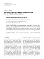
Figure 4: Depiction of PDFs of node separation, with respect to
separation distance state space, at epochs
−1 and 0, taking into ac-
count moves that do and do not result in a link being established.
Nodes are assumed to be uniformly distributed.
r +2v
max
. This is equivalent to saying that the node separa-
tion distances are uniformly distributed on a ring with inner
radius r and outer radius r +2v
max
. The PDF of L
−1
is then
f
L
−1

l
−1

=
⎧
⎪
⎨
⎪
⎩
l
−1

2v
max

r + v
max

, r ≤ l
−1
<r+2v
max
,
0 otherwise.
(31)
The marginal PDF of the initial separation distance for
new links, f
L
0
|new
(l
0
| new link) is equal to the portion of
f
L
0
|L
−1
(l
0
| l
−1

) that intersects the region [r − 2v
max
, r), nor-
malized accordingly. Figure 4 illustrates the relationship be-
tween f
L
−1
(l
−1
), f
L
0
|L
−1
(l
0
| l
−1
)and f
L
0
|new
(l
0
| new link)
showing approximate shapes for the random-walk mobility
model, described in Section 5. Obtaining the PDF f
L
0
|L

−1
(l
0
|
l
−1
) is the same as obtaining the PDF f
L
m+1
|L
m
(l
m+1
| l
m
)with
m
=−1. Thus, we obtain a discretized version of f
L
0
(l
0
)
which is our initial condition vector for new links, P
new
(0),
valid when nodes are uniformly distributed.
The new initial condition vector P
new
(0) can be em-

ployed to determine the persistence of a newly established
link, P
new
(k), in the same way as the link persistence for
a particular initial separation and the network average link
persistence are determined.
Now, the PMF, f
D
(k), of the link duration is given by
f
D
(k) = p
n+1
(k) − p
n+1
(k − 1), (32)
where p
n+1
(k) is the final element of the vector P(k) =
P
new
(0)A
k
pst
. The expected value of the link dur ation can be
determined either from this PMF, or similar to link residual
time, from the fundamental matrix
E
{D }=
n


i=1
p
i
(0)
n

j=1
F
i, j
, (33)
where p
i
(0) are the elements of P
new
(0). (Note that there is
no concept of link duration for a given initial separation and
that the link duration calculated here is effectively the net-
work average.)
4.2. Path-based metrics
Path-based metrics are determined from link metrics using
the assumption that links exist independently of each other.
This is true for a randomly chosen path when nodes move
according to an i.i.d. random process, even though consecu-
tive links in a path share a common node. (It may not be true
when attention is restricted to a particular subset of all pos-
sible paths, such as the shortest-distance path between two
nodes.)
4.2.1. Path availability A(k, h)
For a path with h hops, path availability is the product of

the individual link availabilities of the h hops. If the initial
separation distances for each hop in a particular path are
L
0
(1), , L
0
(h), respectively, the path availability can be cal-
culated using
A

k, h; L
0
(1), , L
0
(h)

=
h

i=1
A

k, L
0
(i)

, (34)
where A(k, L
0
(i)) is given by (23). The network average path

availability for h-hop paths is given by
A(k, h) =

A(k)

h
, (35)
where A(k) is the network average link availability, as defined
in Section 4.1.1.
4.2.2. Path persistence P (k, h)
By using the product of the link persistences for each of the
constituent links, the path persistence is given by
P

k, h; L
0
(1), , L
0
(h)

=
h

i=1
P

k, L
0
(i)


, (36)
where P (k, L
0
(i)) is given by (24). The network average path
persistence for an h-hop path is given by
P (k, h) =

P (k)

h
, (37)
where
P (k) is the network average link persistence, as de-
fined in Section 4.1.2.
4.2.3. Path residual time R(h)
For a particular path, the path residual time is the length of
time that the path continuously lasts without breaking. We
can write the CMF, F
R
(k, h), of the path residual time, as
F
R
(k, h) = 1 − P (k, h) = 1 − P (path lasts ≥ k)
= P (path lasts ≤ k).
(38)
Therefore the PMF of the path residual time can be written
as
f
R
(k, h) = P (k − 1, h) − P (k, h). (39)

The expected value of the path residual time can be expressed
by
E

R(h)

=
∞

k=1
kf
R
(k, h) =
∞

k=1
k

P (k − 1, h) − P (k, h)

.
(40)
Sanlin Xu et al. 9
There is no equivalent of the fundamental matrix method
that was available for link residual time.
4.2.4. Path duration D(h)
To determine the path duration, we need to be precise about
the time that the path commences. We will assume that one
link in the path has just become active, and all other links
are active links with unspecified node separation. That is, the

initial condition vector for one of the links is P
new
(0), and
the initial condition for the remaining links is P
net
(0). The
persistence and all links in the path are considered from the
same point in time. Then, the new path persistence P
new
(k, h)
is given by
P
new
(k, h) =

P (k)

h−1
P
new
(k), (41)
where P
new
(k)isdefinedinSection 4.1.4. The PMF of the
path duration f
D
(k, h) is then
f
D
(k, h) = P

new
(k − 1, h) − P
new
(k, h). (42)
In this section, we have derived exact expressions for the mo-
bility metrics using a probability transition matrix derived
from the PDF of the node separation after one epoch. In
Section 6, we use our c alculations to illustrate the values of
these mobility metrics for the random-walk mobility model.
5. APPLICATION USING RANDOM-WALK
MOBILITY MODEL
The random-walk mobility model (RWMM) is probably the
most mathematically tractable mobility model in use. It de-
scribes the basic node mobility parameters, velocity, and di-
rection of travel, in terms of known probability distribu-
tions. We therefore use the RWMM to illustrate the use of
the MCM-derived expressions for the mobility metrics, from
Section 3.
We assume that each mobile node moves with a velocity
uniformly distributed in both speed V ∼ U[v
min
, v
max
]and
direction Φ ∼ U[0, 2π]. Both the speed and direction change
in each epoch but are constant for the duration of an epoch,
and are independent of each other. The speed has mean
v =
(1/2)(v
min

+ v
max
), and variance, σ
2
v
= (1/12)(v
max
− v
min
)
2
.
This random mobility model is widely used to analyze route
stability in multihop mobile environments [3, 23].
We saw in Section 3 that the movement-related PDF re-
quired for the MCM is f
L
m+1
|L
m
(l
m+1
| l
m
), where l
m
is the
separation distance between a pair of nodes at epoch m.To
obtain this PDF, we must formulate a description of the be-
havior of the relative movement.

5.1. Relative movement between two nodes
To determine the PDF f
L
m+1
|L
m
(l
m+1
| l
m
), we begin with the
PDF of the relative movement between a given pair of nodes,
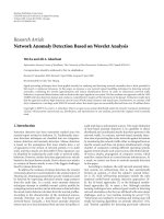
labelled i and j, whose movements are i.i.d. The relationship
between the relative movement vector

X in any given epoch,
and the node velocity vectors

V
i
and

V
j
is

X =

V
j

−

V
i
,asde-
picted in Figure 5.LetX be the random variable representing
Node i at epoch m +1
Node j at epoch m +1
X
V
j
V
i
L
m+1
L
m
L
m+1
X
V
j
Node i at epoch m
Node j at epoch m
Θ
Ψ
Figure 5: Relationship between the node movement vectors

V
i

and

V
j
of nodes i and j, respectively, relative movement vector ,

X,sepa-
ration vector at epoch m,

L
m
, and separation vector after one epoch,

L
m+1
. Solid lines indicate actual vector positions and dashed lines
indicate vectors shifted for illustration purposes. The dotted circles
indicate the loci of possible positions for nodes i and j at epoch
m +1.
the mag nitude of

X, similarly for V
i
and V
j
. The acute angle
Ψ between

V
i

and

V
j
is uniformly distributed in [0, π), and
Ψ, V
i
and V
j
are independent, so we have the joint PDF
f
Ψ,V
i
,V
j

ψ, v
i
, v
j

=
1
12πσ
2
v
. (43)
Using the cosine rule, it can be seen that the relative move-
ment X is related to the random variables V
i

, V
j
,andΨ by
X
=

V
2
i
+ V
2
j
− 2V
i
V
j
cos Ψ. (44)
We use the Jacobian transform [24] to obtain the joint PDF:
f
X,V
i
,V
j

x, v
i
, v
j

=

∂ψ
∂x
f
Ψ,V
i
,V
j

ψ, v
i
, v
j

=
x
6πσ
2
v

2v
2
i
v
2
j
+2v
2
i
x
2

+2v
2
j
x
2
− v
4
i
− v
4
j
− x
4
.
(45)
Then the marginal PDF of the magnitude of the relative
movement can be found via
f
X
(x) =

v
max
v
min
f
X,V
i
,V
j


x, v
i
, v
j

dv
i
dv
j
, (46)
however, there is apparently no closed-form solution to (46).
So, (45)and(46) describe the behavior of the relative dis-
tance X between a given pair of nodes i and j in any one
epoch, given uniform distributions for V
i
, V
j
, Φ
i
,andΦ
j
,as
previously described.
5.2. Conditional PDF of separation distance
The separation vector at epoch m + 1 is the sum of the sep-
aration vector at epoch m and the relative movement vector,

L
m+1

=

L
m
+

X, as shown in Figure 5. The acute angle be-
tween

X and

L
m
is denoted by Θ, as shown in Figure 5.Again
10 EURASIP Journal on Wireless Communications and Networking
we use the Jacobian transform, this time to replace the ran-
dom variables (X, Θ) with the new pair (L
m+1
, Θ). The value
of new variable L
m+1
depends on the given value of L
m
,so
we include the condition in the notation for the new PDF, to
obtain
f
L
m+1
,Θ|L

m

l
m+1
, θ | l
m

=
∂x
∂l
m+1
f
X,Θ
(x, θ)=
∂x
∂l
m+1
f
X
(x) f
Θ
(θ),
(47)
since the magnitude X and the angle Θ are independent. Θ
is uniformly distributed in the interval [0, π]. The PDF f
X
(x)
is given in (46) and can be reexpressed in terms of the new
variables using
X

= L
m
cos Θ ±

L
2
m+1
− L
2
m
sin
2
Θ. (48)
So the new joint PDF is
f
L
m+1
,Θ|L
m

l
m+1
, θ | l
m

=
l
m+1
f
X


l
m
cos θ ±

l
2
m+1
− l
2
m
sin
2
θ

π

l
2
m+1
− l
2
m
sin
2
θ
.
(49)
We then take the marginal PDF with respect to Θ to find the
PDF of L

m
conditioned on L
m+1
:
f
L
m+1
|L
m

l
m+1
| l
m

=

b
a
f
L
m+1
,Θ|L
m

l
m+1
, θ | l
m


dθ. (50)
Thereareseveraldifferent cases for the relative values of L
m
and L
m+1
which decide the expressions for a and b [25].
Again, there is apparently no closed-form solution to this ex-
pression.
Thus, we have the conditional PDF of node separation
distance after one epoch. Note that the assumption of iden-
tical uniform distributions of V
i
and V
j
is not necessary to
this result, so a similar method could be used to determine
the PDF for arbitrarily distributed, independent V
i
and V
j
.
The PDF (50) can be evaluated at discrete points as indi-
catedin(16), to generate expressions for the mobility metrics
for the RWMM.
5.3. Approximation of link residual time
and link duration
While, for the RWMM, it is difficult to determine an exact
expression for the expected value of the node separation after
a given time, it is actually simple to determine the expected
value of its square. Let the initial separation distance between

apairofnodesbel
0
. Then, after k epochs, from [26]and
[27, equation (4.2-11)], the mean square of the separation
distance l
2
k
is given by
E

l
2
k

= l
2
0
+2k

v
2
+ σ
2
v

, (51)
where
v is the mean node speed, and σ
2
v

is the node speed
variance.
5.3.1. Link residual time approximation
The mean-square value of the separation distance monoton-
ically increases with k. When k is sufficiently large, E
{l
2
k
}
will be greater than r
2
. Assuming that the nodes start within
range of each other, as required for link residual time calcu-
lations to be meaningful, we can expect that the first epoch at
which the mean-square value of the separation distance ex-
ceeds r
2
will be approximately equal to the link residual time.
We denote the separation distance at the end of the epoch
when the link is first broken as r + δ, where 0 <δ<2v
max
,
replace k in (51)withE
{R(l
0
)}, and rearrange to give
E

R


l
0

≈
(r + δ)
2
− l
2
0
2

v
2
+ σ
2
v

. (52)
In [28], we show, via simulation, that δ
≈ (2/3)v,andδ is
negligible when l
0
≤ r/2.
To determine the expected value of the network average
link residual time, we use
E
{R}=

r
0

E

R

l
0

f
L
0

l
0

dl
0
, (53)
where f
L
0
(l
0
)isgivenin(8). Thus, the expected value of the
network average link residual time E
{R} is given by
E
{R}=
r
2
+4rδ +2δ

2
4

v
2
+ σ
2
v

. (54)
5.3.2. Link duration approximation
To derive an approximate expression for the link duration,
we combine the approximate expression for the link residual
time in (52) with a linear approximation for the PDF of the
initial link separation illustrated in Figure 4. The probability
that the initial link separation falls in the region [r
−2v
max
, r−
2v] is nonzero but negligible. In fact it can be shown that
f
L
0
|new
(l
0
| new link) is well approximated by
f
L
0

|new

l
0
| new link

≈
⎧
⎪
⎨
⎪
⎩
l
0
− r +2v
2v
2
, r − 2v ≤ l
0
<r,
0 otherwise.
(55)
The expected link duration is then
E
{D }=

r
r
−2v
E


R

l
0

f
L
0
|new

l
0
| new link

dl
0
≈
v(12r − v)
9

v
2
+ σ
2
v

.
(56)
Here we have assumed that 2

v<r.(Ifv ≥ r, the mobility
model can be considered as a nonrandom travelling model
[2, 29].) In Section 6, we compare these approximations to
the exact values obtained from (30)and(33).
5.4. Application to other mobility models
Our framework can be applied to any statistical mobility
model where nodes move in an i.i.d. manner and node
Sanlin Xu et al. 11
separation evolution relies only on the previous relative posi-
tion. In particular it can be applied to the random waypoint
mobility model, since it is shown in [30] that random way-
point is asymptotic mean stationary.
Our framework does not directly apply to determinis-
tic mobility models such as t race-based models. Indeed, the
mobility metrics examined do not make sense with respect
to such models. However, for deterministic models, equiva-
lent average mobility metrics may be of interest. These can
be calculated using our framework by replacing the PDF
f
L
m+1
|L
m
(l
m+1
| l
m
) with the network average movement be-
tween epochs.
6. VERIFICATION AND ANALYSIS OF

CALCULATIONS FOR THE RWMM
Simulations were conducted to verify the theoretical calcula-
tions in Sections 4 and 5.3. Our calculations assume an un-
bounded simulation area. However, it is typical for routing
protocols to be tested using a simulation package such as NS-
2, which confines mobile nodes to a bounded area. Therefore,
we include metric performance results for both bounded and
unbounded areas in our simulations.
6.1. Simulation environment
We ran simulations with each MN moving at a randomly
chosen velocity during each epoch. The speed was uniformly
distributed with v
∈ [0, v
max
], such that σ
2
v
= v
2
max
/3, for var-
ious values of v
max
. The direction was uniformly distributed
in the range [0, 2π). Each MN was equipped with an om-
nidirectional antenna with maximum transmission range of
r
= 100 units.
2
100 MNs start in a square plane of side

1000 distance units. For the bounded scenario, MNs which
reached the boundary were reflected back into the allowed
region for a bounded simulation area. The experiments were
repeated for 2000 trials.
For the path residual time and path duration metrics, we
compared randomly chosen paths with paths found using the
breadth-first search (BFS) algorithm [31] to find the mini-
mum hop path between any given pair of nodes. The differ-
ence between choosing a minimum hop path and a randomly
chosen path is that links in a minimum hop path are likely to
be longer than links in a randomly chosen path. Longer links
are likely to break sooner, so minimum hop paths turn out to
have a shorter residual time and duration than predicted by
our calculations for randomly chosen paths.
6.2. Observations
6.2.1. Availability and persistence
Both the link availability and the link persistence, shown in
Figures 6(a) and 6(b), decrease with increasing simulation
time, and at a greater rate with increasing ratio of mean
2
We use the generic term “units” rather than, say, m or km because it is the
relative and not the absolute distances that are important.
node speed to transmission range v/r. Given the same simu-
lation time and
v/r, the link persistence is much smaller than
the corresponding link availability, as would be expected be-
cause the link availability allows breakage and reestablishing
of links. Further, the path availability and the path persis-
tence, shown in Figures 6(c) and 6(d),dropoff at a greater
rate than the link availability and the link persistence, respec-

tively, for the same mean node speed, as would be expected.
The path availability and the path persistence also drop off
more quickly with an increased number of hops, as there is
more chance of an individual link breaking.
6.2.2. Residual time and duration
In Figures 7 and 8, the expected link (path) residual time and
the expected link (path) duration have been plotted against
(r/v
max
)
2
and r/v
max
, respectively, each showing a linear rela-
tionship. That is,
E
{D } ∝
r
v
max
, E

D (h)

∝
r
v
max
, (57)
E

{R} ∝

r
v
max

2
, E

R(h)

∝

r
v
max

2
. (58)
The relationship in (57) agrees with the experimentally
derived relationship as stated in [7]. As expected, E
{R(h)}
and E{D (h)} are much lower than E{R} and E{D } for the
same communication range to speed ratio. The probability
distributions show that R(h)andD (h) are more concen-
trated near the origin than R and D . Moreover, the link
(path) residual time and the link (path) duration are expo-
nentially distributed, which can be seen in Figures 7(c), 7(d),
8(c),and8(d). This was experimental ly determined in [12],
and theoretically justified in [20].

It can be observed that the expected link (path) dura-
tion is much less than the average expected link (path) resid-
ual time as shown in Figures 7(b), 8(b), 7(a),and8(a),re-
spectively. This is initially a surprise as one would expect the
link (path) duration to be effectively a maximal value of link
(path) residual time. This is because the distribution of the
initial separation of the links differs in the two cases. Mea-
surement of link duration commences when links first form,
that is when nodes first move within transmission range of
each other. The initial separation L
0
is distributed on the an-
nulus, in the range [r
− 2v
max
, r), with greater likelihood of
being close to r than further within the transmission range. If
the nodes continue to move towards each other, the link du-
ration may be long, however, there is a significant probability
that the newly formed link may break immediately, reduc-
ing the average value of link duration. In contrast, the dis-
tribution of the link separation for residual time is nonzero
in the range [ 0, r). The calculation of the average value of
the residual time includes nodes which are extremely close
to each other, a situation which never arises for m any ac-
tive links. So, the residual time values are somewhat artifi-
cially increased. One possible way to remedy this anomaly
12 EURASIP Journal on Wireless Communications and Networking
0 20 40 60 80 100 120
0

0.1
0.2
0.3
0.4
0.5
0.6
0.7
0.8
0.9
1
Time (epochs)
Link availability
Calculated
v
max
= 0.2r,bounded
v
max
= 0.2r, unbounded
v
max
= 0.4r,bounded
v
max
= 0.4r, unbounded
(a)
0 20 40 60 80 100 120
0
0.1
0.2

0.3
0.4
0.5
0.6
0.7
0.8
0.9
1
Time (epochs)
Link persistence
Calculated
v
max
= 0.2r,bounded
v
max
= 0.2r, unbounded
v
max
= 0.4r,bounded
v
max
= 0.4r, unbounded
(b)
0 20 40 60 80 100 120
0
0.1
0.2
0.3
0.4

0.5
0.6
0.7
0.8
0.9
1
Time (epochs)
Path availability
Calculated
3hops,bounded
3 hops,unbounded
3 hops, unbounded, BFS
6hops,bounded
6 hops,unbounded
6 hops, unbounded, BFS
v
max
= 0.2r
(c)
0 20 40 60 80 100 120
0
0.1
0.2
0.3
0.4
0.5
0.6
0.7
0.8
0.9

1
Time (epochs)
Path persistence
Calculated
3hops,bounded
3 hops,unbounded
3 hops, unbounded, BFS
6hops,bounded
6 hops,unbounded
6 hops, unbounded, BFS
v
max
= 0.2r
(d)
Figure 6: Comparison of metric calculations and simulated results for link (path) availability and link (path) persistence. Each MN moves
at a randomly chosen velocity during each epoch, which has uniformly distributed speed in the range [0, v
max
], and uniformly distributed
direction in the range [0,2π). (a) Comparison of calculated and experimental link availability values for both bounded and unbounded
simulation areas. Calculated values are from (23). (b) Comparison of calculated and experimental link persistence values for both bounded
and unbounded simulation areas. Calculated values are from (24). (c) Comparison of calculated and experimental path availability values
for bounded and unbounded simulation areas and the BFS algorithm. Calculated values are from (35). (d) Comparison of calculated and
experimental path persistence values for bounded and unbounded simulation areas and the BFS algorithm. Calculated values are from (37).
would be to exclude separation distances below an appropri-
ately chosen threshold.
6.2.3. Effect of bounded simulation area
In the bounded simulation environment, MNs were “re-
flected” back into the simulation area, if their movement
would otherwise take them outside. In this case, node pairs
near the edge were more likely to remain in transmission

range, and the link (path) availability and link (path) per-
sistence were artificially increased, compared to those for the
unbounded simulation area. Consequently, the link (path)
residual time and the link (path) duration were increased as
well. The experimental results for the bounded area are still
close to the calculated results but, as expected, not as well
matched.
Sanlin Xu et al. 13
0 102030405060708090100
0
10
20
30
40
50
60
70
80
90
100
(r/v
max
)
2
Average link residual time (epochs)
Calculated
Bounded
Approximate
Unbounded
(a)

012345678910
0
10
20
30
40
50
60
70
80
90
100
r/v
max
Expected link duration (epochs)
Calculated
Bounded
Approximate
Unbounded
(b)
0 102030405060
0
0.05
0.1
0.15
0.2
0.25
Time (epochs)
PDF of link residual time
v

max
= 0.2r
Calculated
(c)
0 102030405060
0
0.05
0.1
0.15
0.2
0.25
Time (epochs)
Distribution of link duration
v
max
= 0.2r
Calculated
(d)
Figure 7: Comparison of metric calculations and simulated results for link residual time and link duration. Each MN moves at a randomly
chosen velocity during each epoch, which has uniformly distributed speed in the range [0, v
max
] and uniformly distributed direction in
the range [0, 2π) (a) Comparison of calculated, approximate, and experimental average link residual time values for both bounded and un-
bounded simulation areas. Calculated values are from (30). The approximation is from (54). (b) Comparison of calculated, approximate, and
experimental average link duration values for both bounded and unbounded simulation areas. Calculated values are from (33). The approx-
imation is from ( 56). (c) Comparison of calculated and experimental distributions of the link residual time for an unbounded simulation
area. Calculated values are from (26). (d) Comparison of calculated and experimental distributions of the link duration for an unbounded
simulation area. Calculated values are from (26).
6.2.4. Effect of selecting the shortest path
We used the BFS algorithm to select the shortest path in

the path-based mobility metric simulations. Recall from
Section 4 that independent link failures are assumed for
path-based mobility metrics. For the shortest path, as cho-
sen by the BFS algorithm, however, the hops are correlated.
In this case, the probability of a path failing quickly is higher
due to the commensurate greater hop lengths, on average,
than for a randomly chosen path. The randomly chosen path
will likely have more hops with shorter lengths. Therefore,
using shortest hop paths, the values of mobility metrics de-
crease, as shown in Figures 6 and 8. This demonstrates that
care must be used in applying our calculations to determine
14 EURASIP Journal on Wireless Communications and Networking
0
10 20 30 40 50 60 70 80 90 100
0
5
10
15
20
25
(r/v
max
)
2
Expected path residual time (epochs)
Calculated
3hops,bounded
3 hops,unbounded
3 hops, unbounded, BFS
(a)

012345678910
0
5
10
15
20
25
r/v
max
Expected path duration (epochs)
Calculated
3hops,bounded
3 hops,unbounded
3 hops, unbounded, BFS
(b)
0 5 10 15 20 25 30
0
0.05
0.1
0.15
0.2
0.25
0.3
0.35
0.4
0.45
0.5
Time (epochs)
Distribution of path residual time
3hops,v

max
= 0.2r
Calculated
(c)
0 5 10 15 20 25 30
0
0.05
0.1
0.15
0.2
0.25
0.3
0.35
0.4
0.45
0.5
Time (epochs)
Distribution of path duration
3hops,v
max
= 0.2r
Calculated
(d)
Figure 8: Comparison of metric calculations and simulated results for path residual time and path duration. Each MN moves at a randomly
chosen velocity during each epoch, which has uniformly distributed speed in the range [0, v
max
] and uniformly distributed direction in the
range [0, 2π). (a) Comparison of calculated and experimental average path residual time values for bounded and unbounded simulation
areas and BFS algorithm. Calculated values are from (40). (b) Comparison of calculated and experimental average path duration values
for bounded and unbounded simulation areas and BFS algorithm. Calculated values are from (42). (c) Comparison of calculated and ex-

perimental distributions of the path residual time for an unbounded simulation area. Calculated values are from (39). (d) Comparison of
calculated and experimental distributions of the path duration for an unbounded simulation area. Calculated values are from (39).
path duration in a particular network routing environment
where the method of choosing the paths may adversely affect
the path duration. It also suggests that selecting the short-
est path for routing is likely to have a detrimental effect on
routing performance in MANETs, due to the route discovery
necessitated by premature route breakage.
7. CONCLUSIONS
Frequent changes in network topology caused by mobility
in mobile ad hoc networks impose great challenges for de-
veloping efficient routing algorithms. The theoretical anal-
ysis framework presented in this paper provides a better
Sanlin Xu et al. 15
understanding of network behavior under mobility and
some fundamental work on the issue of path stability. Apart
from the link availability and path availability in previous lit-
erature, we propose the link and path persistences for eval-
uating link and path stabilities. The Markov chain model
used in this paper has enabled us to accurately determine a
series of mobility metrics. Further, we have presented intu-
itive and simple expressions (52)–(56) for the link residual
time and link duration, for the RWMM, which relate them
directly to the ratio between transmission range and node
speed. These calculations are useful for comparison of artifi-
cial mobility behaviors with actual network implementation
scenarios. The analytical results can be readily applied to var-
ious adaptive routing protocols that use corresponding mo-
bility metrics. Our next step is to develop statistical descrip-
tions of other, more realistic, mobility models, and to apply

this framework to them.
In related work [17, 32], we have utilized our analytical
framework to develop adaptive caching strategies that can
be used to optimize existing on-demand routing protocols,
such as DSR and AODV. We employ the path (link) resid-
ual time and path (link) duration as adaptive parameters for
route and link caching schemes in on-demand routing proto-
cols, to reduce tra ffic control overhead and routing delay. We
have also begun investigating clustering schemes in MANETs
using the mobility metrics calculated in this paper.
ACKNOWLEDGMENTS
The authors wish to thank Dr. Leif Hanlen of the National
ICT Australia for his helpful discussions during the develop-
ment of this work, Dr. J. Boleng from Colorado School of
Mines for providing NS-2 source code used for the link du-
ration simulations, and the helpful comments of the various
reviewers.
REFERENCES
[1] J. Boleng, W. Navidi, and T. Camp, “Metrics to enable adaptive
protocols for mobile ad hoc networks,” in Proceedings of the
International Conference on Wireless Networks (ICWN ’02),pp.
293–298, Las Vegas, Nev, USA, June 2002.
[2] W. Su, S J. Lee, and M. Gerla, “Mobility prediction and rout-
ing in ad hoc wireless networks,” International Journal of Net-
work Management, vol. 11, no. 1, pp. 3–30, 2001.
[3] P. Samar and S. B. Wicker, “On the behavior of communica-
tion links of a node in a multi-hop mobile environment,” in
Proceedings of the 5th ACM International Symposium on Mobile
Ad Hoc Networking and Computing (MobiHoc ’04), pp. 145–
156, Roppongi Hills, Tokyo, Japan, 2004.

[4] L. Qin and T. Kunz, “Increasing packet delivery ratio in DSR
by link prediction,” in Proceedings of the 36th Annual Hawaii
International Conference on System Sciences (HICSS ’03),pp.
300–309, Big Island, Hawaii, USA, January 2003.
[5] A. B. McDonald and T. F. Znati, “A mobility-based framework
for adaptive clustering in wireless ad-hoc networks,” IEEE
Journal on Selected Areas in Communications, vol. 17, no. 8,
pp. 1466–1487, 1999.
[6] S. Jiang, Y. Liu, Y. Jiang, and Q. Yin, “Provisioning of adapt-
ability to variable topologies for routing schemes in MANETs,”
IEEE Journal on Selected Areas in Communications, vol. 22,
no. 7, pp. 1347–1356, 2004.
[7] F. Bai, N. Sadagopan, and A. Helmy, “Important: a frame-
work to systematically analyze the impact of mobility on per-
formance of routing protocols for adhoc networks,” in Pro-
ceedings of the 22nd Annual Joint Conference of the IEEE Com-
puter and Communications Societies (INFOCOM ’03), vol. 2,
pp. 825–835, San Francisco, Calif, USA, March-April 2003.
[8] M. Gerharz, C. de Waal, P. Martini, and P. James, “Strategies
for finding stable paths in mobile wireless ad hoc networks,” in
Proceedings of the 28th Annual IEEE International Conference
on Local Computer Networks (LCN ’03), pp. 130–139, Bonn,
Germany, October 2003.
[9] H. M. Jones, S. Xu, and K. L. Blackmore, “Link ratio for ad
hoc networks in a r ayleigh fading channel,” in Proceedings of
the 3rd Workshop on the Internet, Telecommunications and Sig-
nal Processing (WITSP ’04), pp. 252–255, Adelaide, Australia,
December 2004.
[10] S. Jiang, “An enhanced prediction-based link availability esti-
mation for MANETs,” IEEE Transactions on Communications,

vol. 52, no. 2, pp. 183–186, 2004.
[11] A. B. McDonald and T. Znati, “A path availability model
for wireless ad-hoc networks,” in Proceedings of IEEE Wire-
less Communications and Networking Conference (WCNC ’99),
vol. 1, pp. 35–40, Orleans, La, USA, September 1999.
[12] N. Sadagopan, F. Bai, B. Krishnamachari, and A. Helmy,
“PATHS: analysis of PATH duration statistics and their impact
on reactive MANET routing protocols,” in Proceedings of the
4th ACM Interational Sy mposium on Mobile Ad Hoc Network-
ing and Computing (MobiHoc ’03), pp. 245–256, Annapolis,
Md, USA, June 2003.
[13] D. Yu, H. Li, and I. Gruber, “Path availability in ad hoc net-
works,” in Proceedings of the 10th International Conference
on Telecommunications (ICT ’03), vol. 1, pp. 383–387, Tahiti,
Polynesia, February-March 2003.
[14] S. Xu, K. L. Blackmore, and H. M. Jones, “Mobility assessment
for MANETs requiring persistent links,” in Proceedings of Inter-
national Workshop on Wireless Traffic Measurements and Mod-
eling in Conjunction with MobiSys (WiTMeMo ’05), pp. 39–44,
Seattle, Wash, USA, June 2005.
[15] T. Camp, J. Boleng, and V. Davies, “A survey of mobility mod-
els for ad hoc network research,” Wireless Communications and
Mobile Computing, vol. 2, no. 5, pp. 483–502, 2002, special is-
sue on mobile ad hoc networking: research, trends and appli-
cations.
[16] C. Bettstetter, H. Hartenstein, and X. P
´
erez-Costa, “Stochastic
properties of the random waypoint mobility model,” Wireless
Networks, vol. 10, no. 5, pp. 555–567, 2004.

[17] S. Xu, K. L. Blackmore, and H. M. Jones, “Cache timeout
strategies for on-demand routing in MANETs,” in Proceedings
of Workshop on Information Theory and Signal Proocessing with
DSPCS, pp. 153–158, Noosa, Australia, December 2005.
[18] S. Jiang, D. He, and J. Rao, “A prediction-based link availability
estimation for mobile ad hoc networks,” in Proceedings of the
12th Annual Joint Conference of the IEEE Computer and Com-
munications Societies (INFOCOM ’01), vol. 3, pp. 1745–1752,
Anchorage, Alaska, USA, April 2001.
[19] M. Qin, R. Zimmerman, and L. S. Liu, “Supporting multi-
media streaming between mobile peers with link availability
16 EURASIP Journal on Wireless Communications and Networking
prediction,” in Proceedings of the 13th Annual ACM Interna-
tional Conference on Multimedia (MM ’05), pp. 956–965, Sin-
gapore, November 2005.
[20] Y. Han, R. J. La, and A. M. Makowski, “Distribution of path
durations in mobile ad-hoc networks—Palm’s theorem at
work,” in Proceedings of the 16th ITC Specialist Seminar on Per-
formance Evaluation of Wireless and Mobile Systems, Antwerp,
Belgium, August-September 2004.
[21] J. Yoon, M. Liu, and B. Noble, “Random waypoint considered
harmful,” in Proceedings of the 22nd Annual Joint Conference
of the IEEE Computer and Communications Societies (INFO-
COM ’03), vol. 2, pp. 1312–1321, San Francisco, Calif, USA,
March-April 2003.
[22] R. N. Greenwell, N. P. Ritchey, and M. L. Lial, Calculus for the
Life Sciences, Addison-Wesley, Boston, Mass, USA, 2003.
[23] B.AnandS.Papavassiliou,“Anentropy-basedmodelforsup-
porting and evaluating route stability in mobile ad hoc wire-
less networks,” IEEE Communications Letters,vol.6,no.8,pp.

328–330, 2002.
[24] A. Papoulis and S. U. Pillai, Probability, Random Variables and
Stochastic Processes, McGraw-Hill, New York, NY, USA, 2002.
[25] S. Xu, “Mobility metrics for routing in MANETs,” Ph.D. dis-
sertation, Australian National University, Canberra, Australia,
2006.
[26] R. P. Salda
˜
na and M. C. C. Changho, “On random walk mod-
els and Markov chains,” in Proceedings of the 1st Philippine
Computing Science Congress (PCSC ’00), pp. 202–205, Manlila,
Philippines, November 2000.
[27] P. Beckmann, Probability in Communication Engineering,Har-
court, Brace & World, New York, NY, USA, 1967.
[28] S. Xu, K. L. Blackmore, and H. M. Jones, “Link duration calcu-
lation of random walk mobility model in mobile ad hoc net-
works,” Tech. Rep. ANU FEIT 11-02-04, Department of Sys-
tems Engineering, The Australian National University, Can-
berra, Australia, 2004.
[29] W. Su and M. Gerla, “IPv6 flow handoff in ad hoc wireless
networks using mobility prediction,” in Proceedings of Global
Telecommunications Conference (GLOBECOM ’99), vol. 1, pp.
271–275, Rio de Janeireo, Brazil, December 1999.
[30]R.Timo,L.Hanlen,andK.L.Blackmore,“Alowerbound
on network layer control information,” in The European Net-
work of Excellence in Wireless Communications and the Aus-
tralian ARC Communications Research Network (NEWCOM-
ACoRN ’06), Vienna, Austria, September 2006.
[31] T.H.Cormen,C.E.Leiserson,R.L.Rivest,andC.Stein,In-
troduction to Algorithms, McGraw-Hill, New York, NY, USA,

2nd edition, 1998.
[32] S. Xu, K. L. Blackmore, and H. M. Jones, “Practical scheme for
optimizing route-cache TTL in MANETs,” in preparation.