Báo cáo hóa học: " Research Article Channel Impulse Response Length and Noise Variance Estimation for OFDM Systems with Adaptive Guard Interval" docx

Hindawi Publishing Corporation
EURASIP Journal on Wireless Communications and Networking
Volume 2007, Article ID 24342, 13 pages
doi:10.1155/2007/24342
Research Article
Channel Impulse Response Length and Noise Variance
Estimation for OFDM Systems with Adaptive Guard Interval
Van Duc Nguyen,
1
Hans-Peter Kuchenbecker,
2
Harald Haas,
3
Kyandoghere Kyamakya,
4
and
Guillaume Gelle
5
1
Department of Communication Engineering, Faculty of Electronics and Telecommunications, Hanoi University of Technology,
1 Dai Co Viet Stree t, Hanoi, Vietnam
2
Institut f
¨
ur Allgemeine Nachrichtentechnik, Universit
¨
at Hannover, Appelstrasse 9A, 30167 Hannover, Germany
3
School of Engineering and Science, International University Bremen, Campus Ring 12, 28759 Bremen, Germany
4
Department of Informatics-Systems, Alpen Adria University Klagenfurt, Universit

¨
atsstrasse 65-67, 9020 Klagenfurt, Austria
5
CReSTIC-DeCom, University of Reims Champagne-Ardenne, Moulin de la Housse, BP 1039, 51687 Reims Cedex 2, France
Received 5 October 2005; Revised 16 August 2006; Accepted 14 November 2006
Recommended by Thushara Abhayapala
A new algorithm estimating channel impulse response (CIR) length and noise variance for orthogonal frequency-division multi-
plexing (OFDM) systems with adaptive guard interval (GI) length is proposed. To estimate the CIR length and the noise variance,
the different statistical characteristics of the additive noise and the mobile radio channels are exploited. This difference is due to
the fact that the variance of the channel coefficients depends on the position within the CIR, whereas the noise variance of each
estimated channel tap is equal. Moreover, the channel can vary rapidly, but its length changes more slowly than its coefficients.
An auxiliary function is established to distinguish these characteristics. The CIR length and the noise variance are estimated by
varying the parameters of this function. The proposed method provides reliable information of the estimated CIR length and the
noise var iance even at signal-to-noise ratio (SNR) of 0 dB. This information can be applied to an OFDM system with adaptive GI
length, where the length of the GI is adapted to the current length of the CIR. The length of the GI can therefore be optimized.
Consequently, the spectr al efficiency of the system is increased.
Copyright © 2007 Van Duc Nguyen et al. This is an open access article distributed under the Creative Commons Attribution
License, which permits unrestricted use, distribution, and reproduction in any medium, provided the original work is properly
cited.
1. INTRODUCTION
In OFDM systems, the multipath propagation interference is
completely prevented, if the GI is longer than the CIR length,
namely the maximum time delay of the channel. However,
the GI carries no useful information. Therefore, the longer
the GI is, the more the spect ral efficiency will be reduced.
The GI length is a system parameter which is assigned by the
transmitter. However, the CIR length depends on the trans-
mission environment. So, when the receiver moves from one
transmission environment to another, the CIR length must
be changed. The purpose of this paper is to design an OFDM

system with adaptive GI length, where the GI is adapted to
the CIR length of a transmission channel. This avoids unnec-
essary length of the GI, and thus, increases the spectral effi-
ciency of the system. To implement this concept, we have to
deal with the two following problems. Firstly, the CIR length
must be estimated very precisely. Secondly, the network must
be organized in such a way that the information of the cur-
rently estimated CIR length at the receiver can be fed back to
the transmitter to control the GI length.
In a coherent OFDM system, the channel must be esti-
mated for equalization. Generally, even though the channel is
estimated, the CIR length remains unknown. This is because
the estimated CIR is affected by additive noise and by dif-
ferent kinds of interference such as intercarrier interference,
cochannel interference, or multiple-access interference. This
task is more difficult for a time-varying channel, since both
the channel coefficients and the CIR length are changeable.
In the literature, there are some methods to estimate the
CIR length [1–6]. The method described in [1] estimates the
CIR based on the estimated SNR. Similar to this method, the
CIR length is estimated in [2] by comparing the estimated
channel coefficients with a predetermined threshold. The
method in [3] is based on the generalized Akaike information
2 EURASIP Journal on Wireless Communications and Networking
criterion [7]. It was shown in the mentioned reference that
the CIR length is usually underestimated. The method in
[4] is based on the minimization of the mean square error
of the estimated channel coefficients for different predeter-
mined CIR lengths. To apply this method, the channel win-
dow (the range between the minimal and the maximal CIR

lengths) must be known. In [6], the estimation of the CIR
length is based on a given factor R which is defined by the
ratio of the channel variance to the variance of the estimated
channel including the channel variance and the noise vari-
ance. The ratio R is defined in [6] as a constant factor in the
interval [0.9
→ 0.95]. Since the noise variance a nd the chan-
nel variance are unknown, the estimation of the CIR length
basedonagivenratioR does not provide a precise solution.
To overcome the difficulties of CIR length estimation for
OFDM systems in the presence of strong additive noise and
on a time-varying channel, we suggest an auxiliary function
to distinguish the statistical characteristics of the additive
noise and the multipath channel. The difference between the
statistical characteristics of the additive noise and the chan-
nel coefficients lies in the fact that the variance of the true
CIR is distributed only in the area of the true CIR length,
whereas variance of noise per channel tap is uniformly dis-
tributed on the whole length of the estimated CIR. Due to the
relative movement between the receiver and the t ransmitter,
the channel is time-variant. However, it is well known that
the CIR length changes more slowly than the channel coef-
ficients. This is due to the fact that the CIR length depends
mainly on the propagation environment. In practice, a re-
ceiver cannot move from one environment to another, for
example, indoor to outdoor, within less than a second. So,
this time delay can be exploited to improve the channel coef-
ficients, and thus to reduce the influence of the additive noise
on the performance of the proposed algorithm.
The rest of this paper is organized as follows: the auxiliary

function is introduced in Section 2. An algorithm combining
noise variance and CIR length estimation is introduced in
Section 3. Section 4 describes how to calculate the estimated
SNR from the estimated noise variance. The performance of
the proposed method is evaluated in Section 6. Finally, the
paper is concluded in Section 7.
2. INTRODUCTION OF THE AUXILIARY FUNCTION
To establish the auxiliary function, we assume that the chan-
nel is already estimated by a conventional method, for ex-
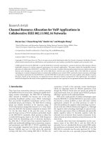
ample, [8]. Figure 1 shows simulation results of an estimated
channel under the presence of strong additive noise (SNR
=
5 dB). The exact CIR length N
P
is equal to 8 sampling inter-
vals and the estimated CIR length N
K
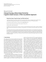
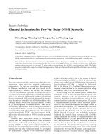
is equal to 15. Figure 2
demonstrates an example of an estimated multipath channel
profile of a time-varying channel.
In the following, we consider the estimated channel co-
efficient
ˇ
h
k,i
corresponding to the ith OFDM symbol and the
kth channel tap index. If we assume that the channel taps
are equidistant and distributed with the sampling interval
t
a

of the system, then the relationship between the chan-
nel tap index k and the corresponding propagation delay is
0
0.2
0.4
0.6
0.8
1
Amplitude of CIR
0 2 4 6 8 10121416
Tap index
Example of an estimated CIR with SNR
= 5dB
True channel
Estimated channel
Figure 1: Estimated channel impulse response distorted by additive
noise.
0
1
2
3
4
ρ(τ, t)
t
Averaging length
13579111315
τ
(
50 ns)
Figure 2: Estimated multipath channel profile of a time-vary ing

channel observed at different observed times.
τ
k
= k ·t
a
. The estimated channel coefficient
ˇ
h
k,i
is composed
of the true channel coefficient h
k,i
and the noise component
n
k,i
, that is,
ˇ
h
k,i
= h
k,i
+ n
k,i
,(1)
where the noise term n
k,i
and the channel coefficient h
k,i
are
statistically independent. The variance of the noise compo-

nent of the tap k is
σ
2
n
[k] = E



n
k,i


2

,(2)
where E[
|n
k,i
|
2
] is the expectation of |n
k,i
|
2
over the OFDM
symbol index i.In(1), the first term is the true channel co-
efficient and its variance depends on its position inside the
Van Du c Ng uyen et al. 3
length of the CIR. The second term is a stationar y additive
noise and its variance is equal in the whole length of the es-

timated CIR. Therefore, the channel tap index is omitted in
the expression of the noise variance, that is, σ
2
n
[k] is replaced
by σ
2
n
.
If an arbitrary value L is supposed to be the true CIR
length, then the new estimated channel

h
L
k,i
coefficients can
be for med by the first L samples of the estimated channel
ˇ
h
k,i
coefficients and are represented by

h
L
k,i
=
⎧
⎨
⎩
ˇ

h
k,i
,0≤ k<L,
0 L
≤ k ≤ N
K
− 1.
(3)
The supposed length L is in the range [1, , N
K
− 1], since
the true CIR length must be larger than zero and is as-
sumed to be smaller than the estimated CIR length. The
mean squared error e(L)between

h
L
k,i
and
ˇ
h
k,i
is
e(L)
= E

N
K
−1


k=0


ˇ
h
k,i
−

h
L
k,i


2

=
E

N
K
−1

k=L


ˇ
h
k,i



2

.
(4)
Thus, e(L) is the cumulation of the average squared magni-
tude of the estimated channel taps from the Lth channel tap
to the last channel tap. It is a function of L, and is hence-
forth named the cumulative function. Substituting
ˇ
h
k,i
from
(1) into (4), it follows that
e(L)
= E

N
K
−1

k=L


h
k,i
+ n
k,i


2


=
N
K
−1

k=L

E



h
k,i


2

+E



n
k,i


2

=
N

K
−1

k=L
ρ
k
+

N
K
− L

σ
2
n
,
(5)
where ρ
k
= E[|h
k,i
|
2
] is the average power of the kth path.
In (5), let e
1
(L) =

N
K

−1
k
=L
ρ
k
be the first term and let
e
2
(L) = (N
K
− L)σ
2
n
be the second term of the cumula-
tive function e(L), it can be seen that e
1
(L) stems completely
from the channel, wh ereas e
2
(L) originates merely from the
noise components. The cumulative function e(L)illustrated
in Figure 3 is a monotonously decreasing function which
does not reveal any information of the CIR length. However,
if the noise-related term e
2
(L) is perfectly compensated by
adding the compensation term Lσ
2
n
to the cumulative func-

tion e(L), then the resulting function decreases only in the
range of the CIR length and it is constant outside this range
(see Figure 4). The breakpoint of the resulting function cor-
responds to the true CIR length. Henceforth, the resulting
function is called the auxiliary function. In practice, the true
noise variance is unknown. Thus, the true noise variance is
replaced by a so-called presumed noise v ariance. Firstly, the
0
N
K
σ
2
n
e(L)
1 N
p
N
K
L
Cumulative function
Channel-related term e
1
(L)
Noise-related term e
2
(L)
Figure 3: The cumulative function e(L).
0
N
K

σ
2
n
f (L)
1 N
p
N
K
L
Compensation term
Channel-related term
Cumulative function
Noise-related term
Auxialiary function in the case
of known noise variance
Figure 4: The auxiliary function f (L) in the case of known noise
variance.
presumed noise variance is initialized to be a possible maxi-
mum value of the true noise variance.
1
Then, the presumed
noise variance will be gradually reduced till it approaches the
true noise variance. This concept will be described precisely
in Section 3.1. According to the compensation of the noise-
related term e
2
(L), the mathematical description of the aux-
iliary function is written as
f (L)
=

N
K
−1

k=L
ρ
k
+

N
K
− L

σ
2
n
+ Lσ
2
pre
,(6)
or
f (L)
= e
1
(L)+e
2
(L)+Lσ
2
pre
. (7)

1
It will be explained later in (9) that the initial value of the presumed noise
variance can be computed from the estimated channel.
4 EURASIP Journal on Wireless Communications and Networking
0
N
K
σ
2
n
f (L)
1
L
(I)
f ,min
N
p
N
K
L
a: σ
2
pre
>σ
2
n
b: σ
2
pre
= σ

2
n
c: σ
2
pre
<σ
2
n
e
1
(L)
e
2
(L)
Lσ
2
pre
Area for detecting the CIR length
Figure 5: The auxiliary function f (L)indifferent cases of the pre-
sumed noise variance σ
2
pre
.
Based on (7), the auxiliary function f (L) is roughly plot-
ted in Figure 5. The characteristics of the auxiliary function
depend on the following cases of the presumed noise vari-
ance.
(a) If the presumed noise variance is larger than the
true noise variance: σ
2

pre
>σ
2
n
, then there exists always a
unique minimum value of the auxiliary function f (L
f ,min
) =
min( f (L)), where L
f ,min
≤ N
P
.Ifσ
2
pre
closes to σ
2
n
, then L
f ,min
also closes to N
P
.
(b) If the presumed noise variance is exactly equal to the
true noise variance, that is, σ
2
pre
= σ
2
n

, then f (L)becomes
f (L)
=
N
K
−1

k=L
ρ
k
+ N
K
σ
2
n
. (8)
In this case, the auxiliary function f (L) is a monotonously
decreasing function within the t rue CIR length, and is equal
to N
K
σ
2
n
outside the true CIR length.
(c) If the presumed noise variance is smaller than the true
noise variance: σ
2
pre
<σ
2

n
, then f (L) is a monotonously de-
creasing function within the whole length of the estimated
CIR, and reaches the minimum value at L
= N
K
− 1.
Based on the characteristics of the auxiliary function
f (L), an algorithm called noise variance and CIR length es-
timation (NCLE) is proposed in the next section.
3. NEW ALGORITHM FOR THE NOISE VARIANCE
AND THE CIR LENGTH ESTIMATION
According to the properties of the auxiliary function, if the
presumed noise variance σ
2
pre
is step by step reduced from
the possible maximum value to the possible minimum value
of the true noise variance, then the curve of f (L)willbe
changed from case (a) to case (c) as depicted in Figure 5.Each
step is considered as one iteration towards the reduction of
the presumed noise variance. The amount Δσ
2
,whichisused
to reduce the presumed noise variance in each iteration, is
called the step size. If this step size is very small in compari-
son with the true noise variance, then case (b) might appear.
Otherwise, case (a) skips directly over to case (c) directly.
When the case (c) appears for the first time, then the pre-
sumed noise variance of the previous iteration is very close

to the true noise variance, and the decision of the estimated
noise variance will be made. The shape of f (L) at the pre-
vious iteration corresponds of course either to case (a) or to
case (b).
If case (a) appears, then the estimated CIR length

N
P
is
assigned to be L
f ,min
,where f (L
f ,min
) = min( f (L)). As ex-
plained in case (a), the estimated CIR length is shorter or
equal to the true CIR length.
Case (b) might appear, if the presumed noise variance
is very close to the true noise variance. Since the theoretical
auxiliary function f (L) of the case (b) is constant over the
range L
= N
P
to N
K
− 1 (see Figure 5), it follows that the
function f (L) does not have unique minimum value like in
the case (a). However, if the minimum value of the auxiliary
function f (L) is still computed by a numerical method, then
a minimum value can be found. This is due to the fact that
the realized auxiliary function is practically not constant in

the interval mentioned above. In this case, the value of L cor -
responding to the minimum value of f (L), that is, L
f ,min
,is
always larger or equal to the true CIR length. The estimated
CIR length can be assigned to be this value, and thus, it is also
larger or equal to the true CIR length.
To ensure that the estimated CIR length is close to the
true CIR length, the procedure of establishing the auxiliary
function f (L) and seeking its minimum value should b e re-
peated N
E
times. A single execution of this procedure is called
an experiment. The estimated CIR length in each experiment
is stored in a vector

L. Analogously, the estimated noise vari-
ance is stored in a vector

N .AfterN
E
experiments, the final
result of the estimated CIR length is the minimum element
of the vector

L. The final estimated noise variance is the av-
erage value of all elements of the vector

N .
3.1. Procedure of the proposed algorithm

Based on above descriptions, the NCLE algor ithm flowchart
is depicted in Figure 6. The algorithm proceeds a s follows.
Step 1. Initial phase of each experiment: determine the ini-
tial value of the presumed noise variance and the step size by
which the presumed noise v ariance will be decreased in each
iteration. The initial value of the presumed noise variance
is the possible maximum value of the true noise variance,
which is determined in the following way. Let us assume that
the true CIR is a Dirac impulse, that is, N
P
= 1. Then, the
first sample of the estimated CIR
ˇ
h
0,i
is the direct path includ-
ing additive noise, the other samples
ˇ
h
k,i
, k = 1, , N
K
− 1,
are completely additive noise components. Hence, the initial
value of the presumed noise variance can be determined by
σ
2
pre
=
N

K
−1

k=1
E



ˇ
h
k,i


2

N
K
− 1
. (9)
Van Du c Ng uyen et al. 5
Set start values for L
avg
, Δσ
2
, s = 1
Set the initial iteration index I
= 1
Read L
avg
measured results of CIR

Calculate start value for σ
2
pre
Establish the auxiliary function f
(I)
(L)
Search L
(I)
f ,min
= L,
where f
(I)
(L) is minimum
L
(I)
f ,min
= N
K
1
True False
Set
σ
2
(s)
n
= σ
2
pre
+ Δσ
2

Set

N
(s)
P
= L
(I 1)
f ,min
, s s +1
Assign
σ
2
(s)
,

N
(s)
P
into vectors
N , L
Set σ
2
pre
σ
2
pre
Δσ
2
I I +1
s

= N
E
False
True
Set

N
P
= min[L]
Set
σ
2
n
= Σ[N ]/N
E
Figure 6: Flowchart of the NCLE algorithm.
It is clear that the true variance σ
2
n
is not larger than σ
2
pre
in
(9). This is due to the fac t that if the CIR length is larger than
one, then it follows in the initial phase that σ
2
pre
consists of a
fraction 1/(N
K

−1) of a part of channel power excluding the
power of the direct path, and the noise variance.
The selection of the step size determines the accuracy of
the estimated noise variance and the estimated CIR length, as
well as the speed of the tracking process. The step size should
be chosen as small as possible to obtain an accurate estimated
noise variance, but not so small that the tracking process runs
slowly.
In Appendix A, it will be proven that if the step size Δσ
2
is chosen to be smaller than the variance of the last channel
tap ρ
N
P
−1
, that is,
ρ
N
P
−1
> Δσ
2
, (10)
then the CIR length can be precisely estimated.
Step 2. Establish the auxiliary function f
(I)
(L), where I rep-
resents the number of iterations in each experiment with the
initial value I
= 1, and seek the minimum value of the aux-

iliary function. These steps are explained in more detail as
follows:
(1) calculate f
(I)
(L) according to (8);
(2) find L
(I)
f ,min
= L,where f
(I)
(L) has a minimum;
(3) compare L
(I)
f ,min
with N
K
− 1. If L
(I)
f ,min
= N
K
− 1,
then go to Step 3. Otherwise, the following steps must
be accomplished:
(i) reduce the presumed noise variance by the step
size Δσ
2
, that is,
σ
2

pre
←− σ
2
pre
− Δσ
2
; (11)
(ii) increase the iteration index I
← I +1;
(iii) repeat Step 2.
Step 3. The decision on the estimated noise variance
ˇ
σ
2
(s)
n
of
the sth experiment is carried out by setting
ˇ
σ
2
(s)
n
to be the av-
erage of the presumed noise variance in the current and the
previous iterations, that is,
ˇ
σ
2
(s)

n
= σ
2
pre
+
Δσ
2
2
. (12)
Store the estimated noise variance obtained from the sth
6 EURASIP Journal on Wireless Communications and Networking
experiment in a vector:
ˇ
σ
2
(s)
n
−→

N
=

ˇ
σ
2
(1)
n
,
ˇ
σ

2
(2)
n
, ,
ˇ
σ
2
(s)
n

. (13)
Step 4. Store

N
(s)
P
= L
(I−1)
f ,min
, which corresponds to the mini-
mum value of the auxiliary function of the previous iteration
in a vector:

N
(s)
P
−→

L
=



N
(1)
P
,

N
(2)
P
, ,

N
(s)
P

. (14)
Increase the experiment index s
← s +1,andrepeatSteps1
to 4 (N
E
− 1) times.
Step 5. Now, each of the vectors

L and

N has N
E
elements. If
the estimated noise variance

ˇ
σ
2
n
of an experiment is very close
to the true value σ
2
n
, then the associated element of

L is a
random number in the interval [N
P
, N
K
−1]. Otherwise, this
element is smaller or equal to the true CIR length, because
case (b) of the auxiliary function does not appear. To ensure
that the estimated CIR length is close to the true CIR length,
the final result of the estimated CIR length is assigned to be a
minimum element of vector

L:

N
P
= min


N

(1)
P
,

N
(2)
P
, ,

N
(s−1)
P

. (15)
It can be proved that if the number of experiments is suffi-
ciently large, then the probability that the CIR length is ex-
actly estimated approaches one (see Appendix B).
Step 6. The estimated noise variances in the single experi-
ments do not differ much from each other, because the step
size is identical in all experiments. To improve the estimation
result, the final result of the estimated noise variance can be
obtained by averaging the results from al l experiments, that
is,
ˇ
σ
2
n
=
1
N

E
N
E

s=1
ˇ
σ
2
(s)
n
. (16)
3.2. Realization of the NCLE
Theoretically, the definition of f (L)in(6) is the sum of the
expectation of

N
K
−1
k
=L
|
ˇ
h
k,i
|
2
and Lσ
2
pre
. Practically, the expec-

tation operation is replaced by an averaging operation over
a finite number of OFDM symbols. That is, the cumulative
function e(L)in(4) and the initial value of the presumed
noise variance in (9) are replaced by
e(L) =

L
avg
−1
i
=0

N
K
−1
k
=L


ˇ
h
k,i


2
L
avg
, (17)
σ
2

pre
=

L
avg
−1
i
=0

N
K
−1
k
=1


ˇ
h
k,i


2

N
K
− 1

L
avg
, (18)

where L
avg
is the averaging length or the number of OFDM
symbols which are taken into account in an averaging oper-
ation. Consequently, the auxiliary function f (L) of the first
iteration is replaced by

f (L) = e(L)+L · σ
2
pre
. (19)
It is clear that if L
avg
is long enough,

f (L) closes to f (L). But it
requires to be short enough, so that the estimated CIR length
is up to date to the current transmission environment. The
whole time requirement per estimate of noise variance and
CIR length is calculated by T
E
= L
avg
·T
S
·N
E
seconds, where
T
S

is the duration of an OFDM symbol in seconds.
4. CALCULATION OF THE SNR BASED ON THE
ESTIMATED NOISE VARIANCE
The aim of this section is to explain how to obtain the SNR
for OFDM systems using a conventional channel estimation
method [8] when σ
2
n
is estimated.
In OFDM systems, the received signal
ˇ
R
l,i
in the fre-
quency domain is given by
ˇ
R
l,i
= S
l,i
H
l,i
+ N
l,i
, (20)
where S
l,i
, H
l,i
,andN

l,i
are the transmitted pilot symbol, the
channel coefficient of the channel transfer function (CTF),
and the noise term in the received signal. The index l denotes
the subcarrier which carries the pilot symbols.
The estimated channel coefficient
ˇ
H
l,i
can be obtained by
dividing the received pilot symbol by the transmitted pilot
symbol as follows:
ˇ
H
l,i
= H
l,i
+
N
l,i
S
l,i
. (21)
We den ote
N
H
l,i
=
N
l,i

S
l,i
(22)
as the noise component in the estimated CTF coefficient.
This noise component is obtained by the DFT of the se-
quence n
k,i
, k = 0, , N
K
−1. The variance of the noise com-
ponents in the estimated CTF is
σ
2
N
= E



N
H
l,i


2

= E






N
l,i
S
l,i




2

. (23)
It can be proved that σ
2
N
and σ
2
n
have the following relation-
ship [9]:
σ
2
N
= N
K
· σ
2
n
. (24)
The power of the transmitted pilot symbols is denoted by

P
P
= E[|S
l,i
|
2
]. Since the noise component and the trans-
mitted pilot symbol are statistically independent, it can be
deduced from (23) that
σ
2
S
= E



N
l,i


2

=
σ
2
N
· P
P
. (25)
The following equation describes the relationship between σ

2
S
and σ
2
n
:
σ
2
S
= σ
2
n
· N
K
· P
P
. (26)
Finally, the SNR is calculated by
SNR
=
P
S
σ
2
S
, (27)
where P
S
is the signal power.
Van Du c Ng uyen et al. 7

Modulator
in baseband
Insert pilot
symbols
Insert
adaptive
guard interval
Inverse
fast Fourier
transform
Digital-
analog
converter
Mobile
channel
Transmitted bit sequence
+
Noise
Received bit sequence
Demodulator
in baseband
Equalizer
Fast Fourier
transform
Remove
adaptive
guard interval
Analog-
digital
converter

CSI
generator
Remove
pilot symbols
Estimated noise variance
NCLE
Channel
estimation
Estimated CIR length
Figure 7: Structure of an OFDM system with adaptive guard interval (illust ration in baseband).
5. STRUCTURE OF AN OFDM SYSTEM WITH
ADAPTIVE GUARD INTERVAL
Figure 7 shows the st ructure of an OFDM system with adap-
tive guard interval, where the NCLE algorithm is applied. So
it provides a reliable information of CIR length for both the
receiver and the transmitter to adjust the GI length adap-
tively. Moreover, the estimated noise variance can be used for
generation of the channel state information (CSI), which can
be exploited to improve channel coding and data equaliza-
tion performance.
Since the CIR length varies slowly, it is not necessary to
adjust the GI length from OFDM symbol to OFDM symbol.
So in a time interval, whereby the CIR length does not sig-
nificantly change, the GI length is kept constant. From this
point of view, the synchronization algorithm based on corre-
lation of the guard interval can be applied for the proposed
OFDM system as in a conventional OFDM system.
To implement the adaptive GI length concept for broad-
casting OFDM systems, a feedback channel is required for
signaling the CIR length information from the receiver to the

transmitter. However, for network working in time-division
duplex (TDD) mode, the estimated CIR length for the down-
link channel is equivalent to that for the uplink channel. This
is due to the fact that the channel is usually reciprocal in a
TDD network. Therefore, when a mobile station or base sta-
tion is in the receiving mode, it will estimate the CIR length
by using the NCLE. The estimated CIR length can be used to
control the GI length when it changes to tr a nsmitting mode.
In this network, the proposed system does not require an ad-
ditional signaling channel.
Due to the use of the GI, the spect ral efficiency of the
system and the achievable data rate are reduced by a fac-
tor η
= T
S
/(T
S
+ T
G
). The SNR is also reduced by this f ac-
tor because of the missmatched filtering effect. In the case
of the adaptive GI, the factor η changes dependent on the
GI length, which is equal to the CIR length. The CIR length
depends again on the transmission environment, where the
communication pair is located. Thus, the gain of the achiev-
able data rate by applying the adaptive GI technique relates
to the location distribution of the active terminals in the net-
work, and their lifetime in each transmission environment. A
quantitative gain in terms of data rate can only be estimated
for a specified scenario. This gain could be significant for a

network covering large areas. In other cases, it could not be
significant, because the CIR length does not change signifi-
cantly.
6. SIMULATION RESULTS
6.1. System parameters and channel model
In our simulation environment, the channel simulated is
adopted from the indoor channel model A described in [10].
The OFDM system parameters are taken from the hiper-
LAN/2 [11]. However, the minimum tap delay (10 nanosec-
onds) of the channel given in [10]doesnotmatchwiththe
sampling interval of the OFDM system (t
a
= 1/B = 50
8 EURASIP Journal on Wireless Communications and Networking
Table 1: Discrete multipath channel profile.
Tap index k Propagation delay τ
k
(ns)
Channel tap power
ρ
k
= E



h
k,i


2


001.0
1500.3714
2 100 0.2445
3 150 0.155
· 10
−1
4 200 0.562 ·10
−1
5 250 0.361 ·10
−1
6 300 1.343 ·10
−2
7 350 4.886 ·10
−3
8 400 2.134 ·10
−3
nanoseconds), and the time spacing between each tap is not
uniform. Therefore, the channel model in this paper is es-
tablished as follows. First, all the channel coefficients which
do not coincide with the sampling position of the system
are interpolated. Then, the channel coefficients defined in
this paper are the channel coefficients of the channel model
A[10], if the corresponding positions of these coefficients
coincide with the sampling positions of the system. Oth-
erwise, the interpolated coefficients are taken. The channel
simulated in this paper is given in Table 1 . It consists of 9
taps. Since the distance between two neighbor taps is equidis-
tant, the maximal CIR length N
P

is 9 samples, which corre-
sponds to 400 nanoseconds. The variance of the last tap is
ρ
N
P
−1
= 2.134 · 10
−3
.
The important OFDM system parameters for simulations
arelistedasfollows:
(i) bandwidth of the system B
= 20 MHz,
(ii) sampling interval t
a
= 1/B = 50 nanoseconds,
(iii) FFT length N
FFT
= 64,
(iv) symbol duration T
S
= 3.2 microseconds,
(v) guard interval length T
G
= 400 nanoseconds.
6.2. Comparison of the proposed technique with
Larsson’s method
In [3], Larsson et al. proposed a method for estimating the
CIR length based on the generalized Akaike information cri-
terion (GAIC). The cost function is established by using the

transmitted pilot symbols denoted as p in [3], the received
pilot symbols as r,andafactorγ,
C(L)
= ln


Wr − diag{p}Wh(L)


2
+ γL, (28)
where W is the DFT matrix [3]. Similar to the proposed
method, L is the presumed CIR length and is assigned to
be the number of the pilot symbols N
K
in the first step. The
presumed CIR length L is decreased step by step till the cost
function reaches its minimum value. The factor γ can be in-
terpreted as a penalty factor which is constant and set to be
0.08. The constant penalty factor is the main drawback of
Larsson’s algorithm. In the proposed algorithm, the penalty
factor is the noise variance σ
2
n
which is adaptively estimated
0
0.5
1
PDF
0

51015
L
Proposed method
Larsson’s method
(a)
0
0.5
1
PDF
0
51015
L
Proposed method
Larsson’s method
(b)
0
0.5
1
PDF
0 5 10 15
L
Proposed method
Larsson’s method
(c)
Figure 8: Comparison results of the PDF obtained by Larsson’s and
proposed methods, true CIR length N
P
= 9 and (a) SNR = 0, (b)
SNR
= 10, and (c) SNR = 40 dB.

according to the channel condition. That is the reason why
the proposed technique provides quite reliable CIR length
information in any range of the SNR. In the case of constant
penalty factor and for a given SNR, the CIR length can be
underestimated, if this factor is too large than a suitable one.
The suitable penalty factor is the one that corresponds to the
actual SNR of the system. In other cases, the CIR length can
be overestimated. This phenomenon can be observed in the
simulation results shown in Figure 8. Larsson et al. reported
also in their simulation results that the CIR length is under-
estimated in most realizations. Their argument for that re-
sult is that some last elements of the CIR are usually very
small. Beside this argument, there is another reason that the
penalty factor γ is selected to be too large for the simulated
SNR in [3].
In order just to demonstrate the advantage of the adap-
tive penalty factor technique, which has b een proposed in
our algorithm, in comparison with the case of constant
penalty factor used in [3], we simplify the auxiliary function
as follows:
f
i
(L) =
N
K
−1

k=0



˘
h
k,i
−

h
L
k,i


2
+ σ
2
n
L. (29)
Van Du c Ng uyen et al. 9
6
5
4
3
2
1
0
1
2
The auxiliary function f (L)(dB)
0246810121416
L
σ
2

pre
= 7.89 10
2
σ
2
pre
= 6.89 10
2
σ
2
pre
= 5.89 10
2
σ
2
pre
= 4.89 10
2
σ
2
pre
= 3.89 10
2
σ
2
pre
= 2.89 10
2
>σ
2

n
σ
2
pre
= 1.89 10
2
<σ
2
n
Figure 9: Simulation results of the auxiliary f unction f (L) in dif-
ferent cases of the presumed noise variance
˘
σ
2
pre
and with step size
Δσ
2
= 10
−2
.
We do not perform the step of time averaging, that is,
L
avg
= 1, and assume that the noise variance is perfectly
known. Under this assumption, the auxiliary function is es-
tablished in every OFDM symbol. The estimated CIR length
corresponds to a value of L that minimizes the auxiliary func-
tion.
Comparison results are illustrated in Figure 8.Thetrue

CIR length corresponds to 9 sampling intervals (N
P
= 9). In
the case of SNR
= 0 dB, the estimated CIR length obtained by
Larsson’s method in almost all realizations is N
K
−1, whereas
the proposed technique gives the results in the range of 3 to
9 sampling intervals. In the case of SNR
= 10 dB, it is clear to
see that the proposed algorithm provides more precise infor-
mation of CIR length than Larsson’s method. This statement
can also be verified in the case of SNR
= 40 dB. Without time
averaging, perfect CIR length information in all realizations
cannot be achieved by the proposed algorithm. However, it
has been shown that the adaptive penalty factor technique
outperforms the constant one. In practice, the penalty factor
is not available, and thus needs to be adaptively estimated.
In the following, we investigate the performance of the com-
plete proposed technique, which combines CIR length infor-
mation with the noise variance estimation.
6.3. NLCE performance in dependence on
the parameter selection
In the following, we consider a system having an SNR of
5 dB. We assume that the powers of the transmitted signal
and the transmitted pilot symbols are normalized. Accord-
30
25

20
15
10
5
0
The auxiliary function f (L)(dB)
0 2 4 6 8 10121416
L
f (L)
e(L)
e
1
(L)
e
2
(L)
Lσ
2
n
Figure 10: Simulation results of the auxiliary function f (L), pro-
vided the noise variance is known (see also (7)).
ing to (27), the noise variance in the received signal corre-
sponding to 5 dB of SNR is σ
2
= 1/(10
5/10
) = 0.3162. Ac-
cording to (26), the noise var iance in the estimated CIR is
σ
2

n
= σ
2
/(N
K
P
P
) = 1.976 · 10
−2
(−17.04 dB). To imple-
ment the auxiliary function, the step size is set to be an arbi-
trary value (e.g., Δσ
2
= 10
−2
). Clearly, this value is relatively
larger than the variance of the last channel tap. The averaging
length L
avg
is set to be 1000 OFDM symbols. The presumed
noise variance is reduced from 7.89
· 10
−2
to 1.89 · 10
−2
,
whereas the true noise variance σ
2
n
is 1.976 · 10

−2
. With this
parameter setup, the auxiliary function is plotted in Figure 9.
Since the condition of the step size in (10) is not fulfilled, the
case (b) in Figure 5 does not occur. The last iteration of the
algorithm is found when the presumed noise variance σ
2
pre
is
reduced to 1.89
·10
−2
. The decision on the estimated variance
is made in the previous iteration, that is,
ˇ
σ
2
n
= 2.89·10
−2
.The
corresponding estimated CIR length is 7 samples, whereas
the true CIR length N
P
is 9 samples. In this case, two last
taps of the CIR are not detected, and the CIR length is un-
derestimated.
If the auxiliary function is established based on the al-
ready know n noise variance (σ
2

n
=−17.04 dB), then the case
(b) of the auxiliary function appears as shown in Figure 10,
where the different terms (e(L), e
1
(L), and e
2
(L)) of the aux-
iliary function are also plotted. It can be seen that the aux-
iliary function is monotonously decreasing within the max-
imal length of the CIR (L<9) and is constant outside the
range of the CIR length (9
≤ L ≤ 15). Since the noise vari-
ance is usually unknown, the case (b) does not occur in prac-
tice. Nevertheless, a close form of the case (b) might occur if
the step size is set to be smal l enough.
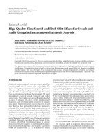
The performance of the NCLE depends on the selection
of three parameters: the averaging length L
avg
, the step size
10 EURASIP Journal on Wireless Communications and Networking
3
4
5
6
7
8
9
10
Estimated channel length

log
10
(ρ
N
P
1
) = 2.67
5 4.5 4 3.5 3 2.5 2 1.5 1
log
10
(Δσ
2
)
(a)
50
40
30
20
10
E
σ
(dB)
5 4.5 4 3.5 3 2.5 2 1.5 1
log
10
(Δσ
2
)
(b)
Figure 11: (a) Estimated CIR length


N
P
versus step size, (b) E
σ
ver-
sus step size.
Δσ
2
, and the number of experiments N
E
. These dependences
are considered as follows. First, the step size of the noise vari-
ance is varied, while the number of experiments and the aver-
aging length are kept constant, N
E
= 10, L
avg
= 1000 OFDM
symbols. The corresponding time duration of an estimation
is T
E
= N
E
· L
avg
· T
S
= 32 milliseconds. The initial value
of the presumed noise variance is determined according to

(18). It can be seen in Figure 11(a) that if the step size Δσ
2
is small enough (less than 10
−3
), then the CIR length is ex-
actly estimated, that is,

N
P
= N
P
. To detect the last element
of the CIR, according to (10), the selection of the step size
must fulfill the following condition: Δσ
2
< 2.134 · 10
−3
(or
log
10
(Δσ
2
) < −2.67), where 2.134 · 10
−3
is the last channel
tap power of the simulated CIR (see Table 1). In the simula-
tions, the step size should be chosen to be less than 10
−3
to
obtain the estimated CIR length which is equal to the true

CIR length. In the range 10
−3
≤ Δσ
2
< 2.134 · 10
−3
, the CIR
length is sometimes underestimated. This is due to the fact
that the last tap of the CIR has relatively small variance, and
therefore it might be neglected in some simulations. When
the step size of the noise variance increases, s ome later are
neglected and the estimated CIR length tends to be shorter.
In order to evaluate the accuracy of the estimated vari-
ance of the noise components, the difference between the
true noise variance and its estimated value E
σ
=|σ
2
n
− σ
2
|
versus the step size is plotted in Figure 11(b).Itcanbecon-
firmed that the smaller the step size is selected, the more ac-
curate the noise var iance can be estimated.
Now, the number of experiments and the step size are
kept constant, for example N
E
= 10, and Δσ
2

= 10
−4
, while
the averaging length is varied. It can be seen in Figure 12(a)
that if the averaging length is larger than 500 OFDM symbols,
6
7
8
9
10
Estimated CIR length
200 400 600 800 1000 1200 1400 1600 1800 2000
L
avg
in OFDM symbols
(a)
18
17.8
17.6
17.4
17.2
17
16.8
Estimated noice variance (dB)
200 400 600 800 1000 1200 1400 1600 1800 2000
L
avg
in OFDM symbols
True noise variance
Estimated noise variance

(b)
Figure 12: (a) Estimated CIR length

N
P
versus averaging length, (b)
estimated noise variance error versus averaging length.
then the exact estimated CIR length can be obtained. The
corresponding time duration of the estimation is T
E
= N
E
·
L
avg
· T
S
= 16 milliseconds.
The estimated noise variance versus the averaging length
is shown in Figure 12(b), where the true noise variance of
σ
2
n
=−17.04 dB is provided for reference. It can be observed
that if the averaging length is large enough, then the esti-
mated value converges to the true noise variance.
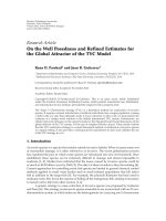
Finally, the step size and the averaging length are kept
constant (Δσ
2
= 10

−4
,andL
avg
= 1000), while the num-
ber of experiments N
E
is varied. The influence of the number
of experiments N
E
on the estimated CIR length

N
P
is illus-
trated in Figure 13(a). The simulation results show that the
CIR length is exactly estimated after three experiments.
It is important to know up to which SNR level the NCLE
algorithm still provides reliable results. This is the aim of
the simulation shown in Figure 13(b). The parameters of the
NCLE are chosen as follows: Δσ
2
= 10
−4
, N
E
= 10. The aver-
aging length L
avg
is varied. In the case of low SNRs, the chan-
nel is strongly impaired. The NCLE algorithm needs there-

fore a long averaging length to detect the true CIR length.
As shown in the simulation results, even though the trans-
mitted signal suffers from 0.0dBofSNR,theCIRlengthcan
be exactly estimated with an averaging length L
avg
over 2000
OFDM symbols. This is because the charac teristics of the
auxiliary function f (L) are not dependent on the noise level.
The corresponding time delay of the algorithm is T
E
= 64
milliseconds.
Van Du c Ng uyen et al. 11
8
9
10
11
12
13
Estimated CIR length
5 1015202530
Number of experiments N
E
(a)
7
7.5
8
8.5
9
9.5

10
Estimated CIR length
012345678910
SNR (dB)
L
avg
= 1000 OFDM symbols
L
avg
= 1500 OFDM symbols
L
avg
= 2000 OFDM symbols
(b)
Figure 13:(a)EstimatedCIRlength

N
P
versus number of experi-
ments N
E
, N
P
= 9, SNR = 5 dB (b) Estimated CIR length

N
P
versus
SNR, N
P

= 9.
The NCLE is also tested in more critical cases. Here, the
channel is time-variant, and the system suffers from strong
additive noise (SNR
= 5 dB). The parameters of the NCLE
are set as follows: L
avg
= 1000, Δσ
2
= 10
−4
, N
E
= 10. The
simulated channel consists of 9 taps as described above, but
now the amplitude of each tap is Rayleigh distributed with
Doppler spread f
D,max
= 50 Hz on each tap. The variance of
each tap is therefore time-variant. In this case, the estimated
CIR length depends heavily on the variation of the variance
of the last tap. If the variance of the last tap is larger than the
step size, then this tap can be detected. Otherwise, it might
be neglected. As shown in Figure 14, the probability for a
correct estimated CIR length is 0.73. Assuming that the av-
eraging length is long enough to obtain an accurate auxiliary
function, and the number of experiments is large enough,
this probability is also the probability that the variance of the
last tap is larger than the step size. The probability that the
last two taps are not detected is the probability that the sum

of the variances of the last two taps is less than the step size,
and so on.
6.4. SystemperformancegainintermsofSERby
applying the NLCE
The perpormance of a conventional channel estimation (CE)
method proposed in [8] can be improved by applying the
NLCE technique. If the CIR length is precisely estimated,
the areas outside the true CIR length are regarded as ad-
ditive noise and can be removed to enhance the CE per-
formance. The improvement of the system performance is
demonstrated in Figure 15, whereas the channel estimator
with the CIR length information obtained by the NLCE out-
performs the conventional one. Moreover, its performance
approaches the case of perfect CE.
7. CONCLUSIONS
In this paper, a novel algorithm for CIR length and noise
variance estimation has been proposed. The proposed algo-
rithm uses an auxiliary funct ion to distinguish the true CIR
length from the estimated CIR. It has been shown by simu-
lation results that this method provides reliable estimation
results in terms of the CIR length and the noise variance,
even though the OFDM systems suffer from the presence
of strong additive noise on a time-variant channel. In ad-
dition, the proposed algorithm has low complexity, since its
implementation requires no matrix operation. The time de-
lay required for an estimate is significantly less than a sec-
ond. It cal l s for a new class of OFDM systems with adaptive
GI length, which optimizes the GI length according to the
transmission environment. Our future research focuses on
the quantitative increase of the data rate which can be gained

by the proposed system in comparison with the conventional
OFDM systems.
APPENDICES
A. CONDITION OF STEP SIZE TO OBTAIN A PRECISE
ESTIMATED CIR LENGTH
As mentioned in Section 3, the step size Δσ
2
should be cho-
sen to be as small as possible to achieve an accurate esti-
mate of the noise variance. But it raises the question of how
small the step size must be, to obtain a precise CIR length.
This question is solved in the following: observing the case
(a) in Figure 5, and taking two special points of f (L)with
L
= [L
f ,min
, N
P
] into account, the associated values of the
auxiliary function are given by
f

L
f ,min

=
N
P
−1


k=L
f ,min
−1
ρ
k
+

N
K
− L
f ,min

σ
2
n
+ L
f ,min
· σ
2
pre
,
f

N
P

=
N
K
−1


k=N
P
−1
ρ
k
+

N
K
− N
P

σ
2
n
+ N
P
· σ
2
pre
,
(A.1)
respectively. From (A.1), the condition f (L
f ,min
) <f(N
P
)is
equivalent to
N

P
−1

k=L
f ,min
−1
ρ
k
<

N
P
− L
f ,min

ΔE, (A.2)
where ΔE
= σ
2
pre
− σ
2
n
. In this case, the last tap numbers
L
f ,min
+1, , N
P
− 1 of the CIR are not detected. In order
12 EURASIP Journal on Wireless Communications and Networking

0
0.1
0.2
0.3
0.4
0.5
0.6
0.7
0.8
0.9
Probability
0246810121416
Estimated CIR length
Figure 14: Estimated CIR length for a time-variant channel.
to detect the position of the last tap of the CIR,
2
that is

N
P
= L
f ,min
= N
P
, the following condition must be fulfilled:
f (N
P
− 1) >f(N
P
). The condition

ρ
N
P
−1
> ΔE(A.3)
follow where ρ
N
P
−1
is the last sample of the delay channel
profile. In the NCLE algorithm, if the case (c) of the auxil-
iary function appears for the first time, the difference of the
presumed noise variance and the true noise variance must be
smaller than the step size, that is, ΔE < Δσ
2
. If the following
condition fulfills
ρ
N
P
−1
> Δσ
2
,(A.4)
then the condition in (A.3) is also met. Equation (10) shows
the condition of the step size to obtain a precise estimation
of the CIR length.
B. PROBABILITY FOR AN EXACT ESTIMATED
CIR LENGTH
The total number of the event


N
(s)
P
= N
P
,(B.1)
which happens r times in any order of N
E
independent ex-
periments, is the total number of the event that the vector

L contains r elements having the value of N
P
. According to
Bernoulli trials [12], this total number is

N
E
r

=
N
E
!
r!

N
E
− r


!
. (B.2)
2
The last tap of the CIR corresponds to the tap which has maximum prop-
agation delay.
10
5
10
4
10
3
10
2
10
1
10
0
SER
0 5 10 15 20 25 30 35 40
SNR (dB)
Conventional CE without CIR length information
CE with estimated CIR length information
Perfect CE
Figure 15: System performance gain in terms of SER by using the
NLCE.
Assuming that the noise variance is perfectly estimated,

N
(s)

P
takes a random value in the range of [N
P
→ N
K
− 1].
Therefore, the probability for the occurrence of the event

N
(s)
P
= N
P
is p = 1/(N
K
− N
P
− 1). It follows that the proba-
bility for r times of the occurrence of the event

N
(s)
P
= N
P
in
any order is calculated by
P

the event L

I
f ,min
= N
P
occurs r times in any order

=

N
E
r

p
r
q
N
E
−r
,
(B.3)
where q
= 1 − p. Since

N
P
= min [

N
(1)
P

,

N
(2)
P
, ,

N
(N
E
)
P
], the
event that

N
P
= N
P
occurs if there is at least one element of
L which is equal to N
P
. The corresponding probability for
the occurrence of the event

N
P
= N
P
is given by

P


N
P
= N
P

=
N
E

r=1

N
E
r

p
r
q
N
E
−r
. (B.4)
Considering the case where the number of experiments N
E
is
large enough, that is N
E

· p · q  1, the right-hand side of
(B.4) can be approximated by [12]
N
E

r=1

N
E
r

p
r
q
N
E
−r
≈
1
σ
√
2π

N
E
1
e
−(x−N
E
p)

2
/2σ
2
dx,(B.5)
where σ
2
= n·p·q. By a suitable substitution, the right-hand
side of (B.5)canbewrittenas[12]
1
σ
√
2π

N
E
1
e
−(x−N
E
p)
2
/2σ
2
dx =
1
σ
√
2π

N

E
−N
E
·p
1
−N
E
·p
e
−(t)
2
/2σ
2
dt.
(B.6)
Van Du c Ng uyen et al. 13
If N
E
· p tends to ∞, that is, N
E
→∞, then the r ight-hand
side of (B.6) is close to one. It can be concluded that
lim
N
E
·p→∞
P


N

P
= N
P

−→
1. (B.7)
The result in (B.7) states that if the number of experi-
ments is sufficiently large, then the probability of an exact
estimation of the CIR length approaches one.
Example for our simulated channel
The CIR length of our channel is N
P
= 9. The length of
estimated CIR is N
K
= 16. The number of experiments is
N
E
= 20. It follows that p = 1/6andq = 5/6. According to
(B.4), the probability of an exact estimated CIR length is
P


N
P
= N
P

=
20


r=1

20
r


1
6

r

5
6

20−r
= 0.9739. (B.8)
REFERENCES
[1] G. E. Bottomley, J C. Chen, and D. Koilpillai, “System and
methods for selecting an appropriate detection technique in a
radiocommunication system,” US patent 6333953B1, Decem-
ber 2001.
[2] J. E. Hudson, “Communication system and methods of
estimating channel impulse responses therein,” US patent
0043887 A1, March 2003.
[3] E. G. Larsson, G. Liu, J. Li, and G. B. Giannakis, “Joint sym-
bol timing and channel estimation for OFDM based WLANs,”
IEEE Communications Letters, vol. 5, no. 8, pp. 325–327, 2001.
[4] J H. Chen and Y. Lee, “Joint synchronization, channel length
estimation, and channel estimation for the maximum likeli-

hood sequence estimator for high speed wireless communi-
cations,” in Proceedings of the 56th IEEE Vehicular Technology
Conference (VTC ’02), vol. 3, pp. 1535–1539, Vancouver, BC,
Canada, September 2002.
[5] P. P. Moghaddam, H. Amindavar, and R. L. Kirlin, “A new
time-delay estimation in multipath,” IEEE Transactions on Sig-
nal Processing, vol. 51, no. 5, pp. 1129–1142, 2003.
[6] Y. Zhao and A. Huang, “A novel channel estimation method
for OFDM mobile communication systems based on pilot sig-
nals and transform-domain processing,” in Proceedings of the
47th IEEE Vehicular Technology Conference (VTC ’97), vol. 3,
pp. 2089–2093, Phoenix, Ariz, USA, May 1997.
[7] H. Akaike, “A new look at the statistical model identification,”
IEEE Transactions on Automatic Control,vol.19,no.6,pp.
716–723, 1974.
[8] P. H
¨
oher, “TCM on frequency-selective land-mobile fading
channels,” in Proceedings of the 5th Tirrenia International
Workshop on Digital Communications, pp. 317–328, Tirrenia,
Italy, September 1991.
[9] C S. Yeh and Y. Lin, “Channel estimation using pilot tones in
OFDM systems,” IEEE Transactions on Broadcasting, vol. 45,
no. 4, pp. 400–409, 1999.
[10] J. Medbo and P. Schramm, “Channel Model for HiperLAN/2
in Different Indoor Scenarios,” ETSIEPBRAN3ERI085B, March
1998.
[11] ETSI Technical Specification TS 101 475 V1.1.1 (2000-04)
HIPERLAN Type 2; Physical (PHY) layer. 2000.
[12] A. Papoulis, Probability, McGraw-Hill, New York, NY, USA,

3rd edition, 1991.