Báo cáo hóa học: " Research Article Polarization Behavior of Discrete Multipath and Diffuse Scattering in Urban Environments " pot

Hindawi Publishing Corporation
EURASIP Journal on Wireless Communications and Networking
Volume 2007, Article ID 57980, 16 pages
doi:10.1155/2007/57980
Research Article
Polarization Behavior of Discrete Multipath and Diffuse
Scattering in Urban Environments at 4.5 GHz
Markus Landmann,
1
Kriangsak Sivasondhivat,
2
Jun-Ichi Takada,
2
Ichirou Ida,
3
and Reiner Thom
¨
a
1
1
Electronic Measurment Research Lab, Institute of Information Technology, Ilmenau University of Technology,
P.O. Box 100 565, 98684 Ilmenau, Germany
2
Department of International Development Engineering, Takada Laboratory, Graduate School of Eng ineering,
Tokyo Institute of Technology, Tokyo 152-8552, Japan
3
Fujitsu Limited, Tokyo 105-7123, Japan
Received 13 April 2006; Revised 7 November 2006; Accepted 15 November 2006
Recommended by Rodney A. Kennedy
The polarization behavior of the mobile MIMO radio channel is analyzed from polarimetric double-directional channel mea-
surements, which were performed in a macrocell rural environment in Tokyo. The recorded data comprise non-line-of-sight,

obstructed line-of-sight, and line-of-sight conditions. The gradient-based maximum-likelihood estimation framework RIMAX
was used to estimate both specular and dense multipath components. Joint angular-delay results are gained only for the specular
components. The dense multipath components, which may be attributed to diffuse scattering, can be characterized only in delay
domain. Different characteristics describing the polarization behavior and power-weighted cross- and copolarization ratios for
both types of components are introduced. Statistical analysis of long measurement track segments indicates global trends, whereas
local analysis emphasizes specific behavior such as polarization dependency on angle of incidence in streets and under shadowing
conditions. The results also underline the importance of modeling changing and transient propagation scenarios which are cur-
rently not common in available MIMO channel models.
Copyright © 2007 Markus Landmann et al. This is an open access article distributed under the Creative Commons Attribution
License, which permits unrestricted use, distribution, and reproduction in any medium, provided the original work is properly
cited.
1. INTRODUCTION
Efficient design of MIMO transmission systems requires a
thorough understanding of the multidimensional structure
of the mobile radio channel. Initially, research was aimed
at the spatiotemporal channel structure at base-station side
only. The appearance of MIMO systems forced a more
detailed description of the mobile radio channel at both
transmitter a nd receiver sides including directions of ar-
rival and departure. Recent simulations [1, 2]andmea-
surements [3–6] showed that the capacity of MIMO sys-
tems can be further enhanced if the polarimetric dimen-
sion is exploited. Moreover, dual polarimetric antennas can
be colocated (e.g., patch antennas), which is a space- and
cost-effective alternative to two spatially separated anten-
nas with the same polarization. The draw back of the ex-
isting results (as mentioned above) is to consider the an-
tennas as a part of the radio channel. There was no at-
tempt to separate the channel characteristics from anten-
nas influence in both the measurement and simulation

cases.
The aim of our work is measurement-based paramet-
ric channel modeling (MBPCM) [7]. The idea behind this
method is to deduce a parametric model of the MIMO chan-
nel that is (within well-defined limits) independent from the
antennas used during the measurement. This offers the pos-
sibility to emulate the MIMO transfer properties of arbi-
trary antenna arrays (again within well-defined limits) by
reconstructing the hypothetical antenna response from the
estimated channel parameters. The key technologies to es-
timate the individual path parameters, removed from the
antenna influence, are high-resolution parameter estimation
[8–10] and precise antenna calibration [11]. There are only a
few dual polarized and double-directional channel measure-
ments described in the literature where these algorithms are
applied and the estimated parameters are analyzed (see [12]
MIMO), (see [13, 14] SIMO). We are using the gradient-
based maximum-likelihood estimation framework RIMAX
2 EURASIP Journal on Wireless Communications and Networking
[10] that estimates both specular and dense multipath com-
ponents. However, joint angular-delay results are gained only
for the specular components. The dense multipath compo-
nents, which may be attributed to diffuse scattering, can
be characterized only in delay domain. We present statisti-
cal analysis of sets of segments that indicate global trends,
whereas local analysis emphasizes specific behavior such as
polarization on angle of incidence in streets and under shad-
owing conditions. The results underline the importance of
modeling of evolving and transient propagation scenarios,
which is currently not common in available MIMO channel

models. This supports the current discussions in propaga-
tion modeling community [15, 16], which indicates also a
deficiency in modelling of polarization.
The paper is organized as follows: Section 2 gives a brief
review of the RIMAX parameter estimation framework. In
Section 3, we present the sounder and data processing system
that were used throughout the measurement campaign. An
overview on the propagation environment and a first general
classification of the estimated results are given in Section 4.
Section 5 discusses the different parameters and their defi-
nitions describing the polarization behavior of the channel.
In Section 6, the statistical analysis along sets of segments of
the measurement run and local analysis results are discussed.
Finally, local results with specific behavior are pinpointed.
2. CHANNEL CHARACTERIZATION
In case of the experimental channel characterization, anten-
nas or antenna arrays at the BS and MS are part of the mea-
sured links. Since we want to char acterize the channel inde-
pendent from the used antenna arrays, high-resolution pa-
rameter estimation algorithms are applied to the measure-
ment data. In our contribution, we use the gradient-based
maximum-likelihood parameter estimation algorithm RI-
MAX [10, 17]. The appropriate data model comprises two
components which can be handled separately throughout the
estimation procedure. The first part is deterministic and re-
sults from specular-like reflection. Each specular component
(SC) k is characterized by its parameters direction of de-
parture (DoD) ϕ
Tk
, ϑ

Tk
(azimuth and elevation), time de-
lay of arrival (TDoA) τ
k
, Doppler shift α
k
, direction of ar-
rival (DoA) ϕ
Rk
, ϑ
Rk
, and the four complex polarimetric path
weights γ
hh,k
, γ
hv,k
, γ
vv,k
, γ
vh,k
, where the first subscript indi-
cates the polarization at the BS side and the second at the MS
side (Figure 1(b)). The vector of the vertical (v) polarization
is parallel to the vector

e
θ
and the vector of the horizontal (h)
polarization is parallel to the vector


e
φ
of the spherical coor-
dinate system. Furthermore, the RIMAX calculates the vari-
ances σ
ϕ
Tk
, σ
ϑ
Tk
, σ
τ
k
, σ
α
k
, σ
ϕ
Rk
, σ
ϑ
Rk
, σ
{γ
hh,k
}
, σ
{γ
hh,k
}

, σ
{γ
vv,k
}
,
σ
{γ
vv,k
}
, σ
{γ
hv,k
}
, σ
{γ
hv,k
}
, σ
{γ
vh,k
}
,andσ
{γ
vh,k
}
of each path
based on the Fischer information matrix [10]. Hereby, the
estimated variances are used to verify the estimation results
of the kth path. The relative variances of the path weights are
calculated, w here a path with a relative variance better than

−3 dB is considered as reliable and paths with a worse rela-
tive variance are dropped. This threshold is reasonable since
a relative variance of
−3 dB stands for equal signal power
00.20.40.60.81
125
120
115
110
105
100
Normalized τ
pdp (dB)
10 log 10(α
0
)
10
log 10(α
1
)
β
d
τ
n
(a)
hh
vv
BS
MS
γ

hh,k
, θ
dsshh
γ
hv,k
, θ
dsshv
γ
vh,k
, θ
dssvh
γ
vv,k
, θ
dssvv
(b)
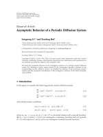
Figure 1:ModeloftheDMC(a),SCpolarizationandDMCpolar-
ization schematic (b).
and noise power. In case of the SCs, the complex polarimet-
ric pathweights are independent from the used measurement
antennas, that is, since we estimate the DoD and DoA, we are
able to exclude the effect of the polarimetric antenna beam
patterns.
The second part of the data model represents the dense
multipath components (DMC) that mainly result from dis-
tributed diffuse scattering. The DMCs are considered as the
remaining complex impulse responses after removing the
contribution of the reliable estimated SCs and measurement
noise. As an extension to the estimation process in [17], the
distribution of the DMC,

α(τ)
=
⎧
⎪
⎪
⎪
⎪
⎪
⎨
⎪
⎪
⎪
⎪
⎪
⎩
α
0
, τ<τ
n
,
1
2
α
1
, τ = τ
n
,
α
0
+ α

1
· e
−β
d
·(τ−τ
n
)
, τ>τ
n
,
(1)
shown in Figure 1(a) is estimated independently for all four
polarization combinations from the corresponding mean
power delay profile (PDP). In the following, we describe the
calculation of these four PDPs. The subtraction of the spec-
ular components from the vector-valued measured impulse
responses h
i,xy
leads to the remaining complex impulse re-
sponses h

i,xy
of all i, xy channels, where x specifies the port
polarization at BS side, y specifies the port polarization at the
Markus Landmann et al. 3
Table 1: Measurement system.
MIMO channel sounder RUSK Fujitsu [18]
Tx power at the antenna ca 2.8 W
Carrier frequency/wavelength 4.5 GHz/λ
= 6.67 cm

Measurement bandwidth 120 MHz
Maximum multipath delay 3.2 μs chosen according to the environment
Number of multiplexed Tx/Rx ports 16 Tx/96 Rx
Total number of MIMO channels 1536
Measurement time of one snapshot 10 milliseconds
Time between 2 snapshots 1.5 seconds
Tx/Rx synchronization Rubidium reference
Base station (Tx side)
4-by-2 element
polarimetric uniform rectangular patch array (PURPA)
Mobile station (Rx side)
24-by-2 element
stacked polarimetric uniform circular patch array (SPUCPA)
XPD [19, equation (13)] Tx/Rx array 13 dB, , 15 dB/10 dB, ,14dB
MS, side and i indicates one channel of all available channels
I with the polarization combination xy. Each port of the an-
tenna ar ray has been designated either as horizontal or verti-
cal. Consequently, x and y are either h or v. To compensate
the effect of the antenna beam patterns at least partly (as no
directional information is considered) for the DMC, h

i,xy
is
divided by the mean ga ins g
i,x
and g
i,y
(3) of the correspond-
ing Tx and Rx port,
h


i,xy
=
h

i,xy
√
g
i,x
· g
i,y
. (2)
The mean gain
g
i,q
=
1
S
·
n
2

n=n
1
m
2

m=m
1



b
i,q
(n · Δϕ, m · Δϑ)


2
· sin (m · Δϑ)
(3)
is calculated from the measured beam pattern b
i,q
(ϕ, ϑ)for
polarization q,whereq is chosen equal to the port polariza-
tion x or y. This means that the cross-polarization term of
the port is neglected. The indices n
1
, n
2
and m
1
, m
2
specify
the azimuth and coelevation ranges, and S
= N · M the to-
tal number of samples that are used for the calculation of the
mean ga in with N
= n
2
− n

1
+1andM = m
2
− m
1
+1.
Using this approach, the assumption has been made that the
DMCs are uniformly distributed in the chosen azimuth and
coelevation ranges. In our analysis, we observed that after re-
moving the contribution of the specular propagation paths
from the measured complex impulse responses the, power
delay-azimuth profile of the remaining complex impulse re-
sponses has only a few directional information in the MS az-
imuth (similar observations were found in [20]). Therefore,
the ranges at the MS side are chosen between 45
◦
to 135
◦
in coelevation with respect to the surrounding area and be-
tween
−180
◦
to 180
◦
in azimuth. At the BS side, it was found
that it is reasonable to limit the range to the broadside di-
rection, where the azimuth range is chosen between
−70
◦
to

70
◦
and the coelevation range between 80
◦
to 140
◦
. The val-
ues Δϕ, Δϑ are the corresponding step sizes in azimuth and
coelevation that are chosen to (1
◦
).
The four parameter vectors of the DMCs θ
dsshh
, θ
dsshv
,
θ
dssvh
,andθ
dssvv
(Figure 1(b)), composed of the parame-
ters θ
dssxy
= [α
0,xy
, α
1,xy
, β
d,xy
, τ

n,xy
], are estimated from the
mean PDP ρ
xy
,
ρ
xy
=
1
I
I

i=1


h

i,xy


2
(4)
of the corresponding polarization combination xy.
3. MEASUREMENT TECHNIQUE
AND DATA PROCESSING
The configuration of the measurement system is summarized
in Table 1. We u sed well-calibrated antenna arrays (manufac-
tured by IRK Dresden [21]) at both link ends, which al low us
to estimate the cross-polarization ratio (XPR) of the SCs up
to

±40 dB. This limitation is c aused by the usage of a refer-
ence horn antenna with a cross-polarization discrimination
(XPD) of 40 dB during the calibration of the Rx and Tx an-
tenna arrays. For the DMCs, the maximum resolvable XPR
of the channel is limited by the XPD of the antenna array el-
ements, given in Tabl e 1. Note that the XPD is a property of
the antenna element, whereas the XPR describes the polar-
ization behavior of the channel.
4 EURASIP Journal on Wireless Communications and Networking
Table 2: Measurement environment.
Environment macrocell
BS (Tx) height 35 m
MS (Rx) height
1.6 m
Building heights around Rx
2-3 floors, mostly residential area
Total measurement route
490 m (ca 2000 snapshots)
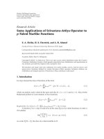
Number of measured segments
45 (see Figure 2)
For the purpose of the offline measurement data process-
ing, by using the RIMAX algorithm, c a 10 PCs are organized
in a batch processing system. To process the total amount of
measurement data, the system was continuously running for
3weeks.
4. MEASUREMENT DESCRIPTION AND
ENVIRONMENT CHARACTERIZATION
In Section 4.1, we give a description of how and where the
measurements were performed. Additionally, background
information is presented on the total power of the estimated

SCs and their path length spread at each measurement posi-
tion (Section 4.2).
4.1. General description
The measurements were performed in a macrocell environ-
ment. Tabl e 2 summarizes the basic information of the sce-
nario. The same system setup and measurement procedure
are applied during the entire campaign, where we used only
one BS (Tx) position while moving to different MS (Rx) po-
sitions. The measurement route is divided in segments of
10 meters. In Figure 2, the significant positions like corners
are labeled with crosses. Each segment is measured in the
same way: 10 static snapshots at the start position, ca 40
snapshots while moving to the next position (i.e., an approx-
imate speed of 25 cm/snapshot), 10 static snapshots at the
end. The measurements are carried out in the neighborhood
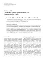
of Minami-Senzoku, Ota-Ku, Tokyo (Figure 3), where the
transmit antenna array (BS) is placed over roof top at a 10-
floor high building in the nearby campus of the Tokyo Insti-
tute of Technology. The receive antenna array (MS) is placed
at a cart around 1.6 m above the street, where the buildings
in the surrounding residential area are between two and three
flours high.
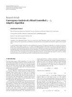
4.2. Environment characterization
The data model used comprises the two components SC and
DMC. For an analysis of the results related to these two com-
ponents, we will indicate the percentage of total power that is
estimated as SC. Figure 4 shows the total specular power as a
percentage at each point.
(i) In the line-of-sigh t (LOS) case, moving from position
Rx1 to Rx6 (see Figure 2), the total specular power rep-

resents around 95% of the signal power.
200 150 100 50 0 50
50
100
150
200
250
Rx x (m)
Rx y (m)
Rx19
Rx27
Rx1 Rx6
Rx38
Tx
Figure 2: Map of macrocell measurement site.
Rx19
Rx27
Rx1
Rx6
Rx38
Figure 3: Picture taken from Tx in the direction of Rx6 macrocell.
(ii) The measurements between position Rx6 and Rx19
are mostly non-line-of-sight (NLOS) with a total SC
power of around 55% to 65%. However, at some po-
sitions, the specular power increases to up to 80%,
which is mainly caused by strong single bounce scat-
tering and obstr ucted line of sight (OLOS). In the par-
allel street between positions Rx27 and Rx38, we ob-
serve similar behavior.
(iii) In the street between position Rx19 and Rx27, the

portion of SCs is almost constant (around 55%). All
measurements here were taken under NLOS condi-
tions. Furthermore, strong single bounce reflections
and OLOS are rare.
(iv)ThemeasurementsbetweenRx38andRx6aredom-
inated by strong single-bounce scattering and OLOS
around the corner of Rx6. The total SC power is be-
tween 65% to 85%.
Plotting the CDF of the specular power for all measurements
(Figure 5), it is apparent that a strong relation exists between
the conditions LOS, OLOS, NLOS, and this parameter.
Markus Landmann et al. 5
50 0 50
80
100
120
140
160
180
200
Rx x (m)
Rx y (m)
55
60
65
70
75
80
85
90

95
Figure 4: Specular power macrocell color-coded in %.
50 60 70 80 90 100
0
20
40
60
80
100
Specular power (%)
CDF (%)
NLOS
LOS
OLOS
LOS
and
strong single-
bounce reflections
Figure 5: CDF of the specular power of the entire route.
To distinguish between local scattering around Rx and far
scattering, the path length spread of the SCs and DMCs is
discussed, which is equivalent to the estimated delay spread
multiplied by the speed of light. Figure 6 shows the path
length spread at each position. It is noted that these values in-
crease drastically around corner Rx19. The causes for that be-
havior are some far clusters, of which 2 clusters are indicated
by arrows in Figure 6. All other regions are dominated by lo-
cal scattering.
The far clusters were localized on basis of estimated an-
gles of the SCs at the BS and MS sides (see Figure 7). Each

path is plotted with half of the path length from Tx and Rx in
the scenario. The colors indicate the total power of a path
in dB. In Figure 8, the CDFs of the path length spread of
the SCs and DMCs are compared. The path length spread of
the DMCs is calculated from the parameter β
d
,whichcorre-
sponds to the coherency bandwidth and which is inversely
proportional to the delay spread. For the DMC, a smaller
variation is observed compared to the SCs. We conclude that
the DMC process is mainly influenced by local scattering.
The authors abstain from a detailed discussion of the es-
100 50 0 50
0
50
100
150
200
Rx x (m)
Rx y (m)
50
100
150
200
2
1
Figure 6: Path length variation in m, where the arrows indicate the
position of far clusters (no. 2 not on the map).
140
135

130
125
120
115
110
105
Tx
Rx
Figure 7: DoA, DoD, and TDoA (as length) for all paths at Rx19.
timated angular parameters and far clusters (can be found
in [22]). The angular parameters are used in Section 6.3 to
identify the cause of specific channel characteristics.
5. HOW TO DEFINE THE POLARIZ ATION BEHAVIOR
OF THE CHANNEL
A lot of publications on XPR exist, but different defini-
tions were found. With the following discussion, the authors
6 EURASIP Journal on Wireless Communications and Networking
0 50 100 150 200 250
0
20
40
60
80
100
Path length variation (m)
CDF (%)
Far scattering
Local scattering
SC
DMC

Figure 8: CDF of the path length variation.
would like to point out the difficulties of a comparison of
various published results. The XPR is basically defined as
the power ratio between the copolarization and the cross-
polarization. In [23], the power ratio between P
qq
and P
qp
at the MS side, respectively, P
pq
at the BS side,
XPR
MS
q
= 10 · log
10

P
qq
P
qp

(dB),
XPR
BS
q
= 10 · log
10

P

qq
P
pq

(dB),
(5)
is used, where q and p can be either horizontal or vertical. To
calculate the powers P
qq
, P
qp
,orP
pq
, the powers of all qq, qp
or pq channels are added up, for example,
P
qq
=
I

i=1


h
H
i,qq
· h
i,qq



,(6)
whereas the column vector h
i,qq
is the ith complex impulse
response w ith the polarization qq. Using this definition, a
reliable estimated XPR is limited to the XPD of the single-
antenna elements.
Another approach uses beam forming or high-resolution
parameter estimation to detect individual r ays/paths. Here,
two definitions can be found, the XPR of a single path k [13]:
XPR
MS
q,k
(s) = 10 · log
10





γ
qq,k
(s)
γ
qp,k
(s)





2

(dB),
XPR
BS
q,k
(s) = 10 · log
10





γ
qq,k
(s)
γ
pq,k
(s)




2

(dB),
(7)
where s is the snapshot index, and the narrowband XPR of
the L
c

paths of a cluster c [24]:
XPR
MS
q,c
(s) = 10 · log
10






L
c
n=1
γ
qq,n,c
(s)

L
c
n=1
γ
qp,n,c
(s)




2


(dB). (8)
Using these definitions, a reliable estimation of the XPR
of a cluster or the SCs is limited to the XPD of the ref-
erence horn antenna during the antenna array calibration
(see Section 3) in the case of double-directional measure-
ments. This is in contrast to, for instance, sing le-directional
measurements. Due to the fact that a single Tx antenna is
used, the angle-of departure cannot be resolved, so com-
pensation for angle dependent XPD is not possible. As a
result, a reliable estimation of the XPR is limited to the
XPD of the transmit antenna, which normally varies be-
tween 8 dB and 20 dB depending on the direction of depar-
ture.
In the following, we define the parameters which are
used during the analysis (Section 6) illustrated with exam-
ples from the measurement segments Rx19 to Rx27. The ba-
sic par ameters are defined for both, the BS and MS sides,
whereas the distributions are only shown for the MS parame-
ters. In Section 5.1, the XPR distribution based on (7)forSCs
and DMCs are discussed, whereas in Section 5.2 the power-
weighted XPR is defined.
5.1. XPR distribution
Definition (7) describes how a single propagation path has to
be modeled in terms of the XPR regardless of the importance
of the path in terms of its total received power.
Figures 11 and 12 show the PDFs of the XPR
MS
h
and

XPR
MS
v
of the SCs for the chosen measurement segment Rx19
to Rx27. The best fit to the normal distribution is plotted
in the PDF of the measurement. The expectation and stan-
dard deviation of the measurement agree with those of the
fitted distribution. This agreement can be observed also for
the other segments (not shown).
For a better understanding of the polarization behavior,
we analyze the copolarization ratio or the ratio of the total re-
ceived or transmitted vertical power to the horizontal power
P
MS
v/h
or P
BS
v/h
(9)(Figure 13)aswell:
P
MS
v/h,k
(s) = 10 · log
10



γ
vv,k
(s)



2
+


γ
hv,k
(s)


2


γ
hh,k
(s)


2
+


γ
vh,k
(s)


2


(dB),
P
BS
v/h,k
(s) = 10 · log
10



γ
vv,k
(s)


2
+


γ
vh,k
(s)


2


γ
hh,k
(s)



2
+


γ
hv,k
(s)


2

(dB).
(9)
To describe the polarization behavior of the DMCs, we apply
definition (7) like in the case of the SCs. Therefore, we calcu-
late a sampled version of the DMC distribution (cf. (1)) for
all four polarization combinations. We use the distance
Δτ
=
1
B
(10)
between two samples, where B is the measurement band-
width. To calculate the XPR of the DMC, the samples k
DMC
=
1, , K
DMC
(K

DMC
∈ N) are used. These samples are in the
Markus Landmann et al. 7
range of the largest delay spread of the four DMC processes:

min

θ
β
d

−1
Δτ
<K
DMC
≤
Δτ +

min

θ
β
d

−1
Δτ
, (11)
where θ
τ
n

and θ
β
d
are vectors that include the estimates of τ
n
and β
d
of all four polarization combinations. The first sample
in the delay τ is defined by the minimum base delay τ
n min
=
min(θ
τ
n
). To use (7) for the DMC,
γ
k
DMC
,xy
=

α
xy

τ
nmin
+

k
DMC

− 1

·
Δτ

(12)
is defined. The calculated XPR of the DMC, using this def-
inition, is only valid for values smaller than the XPD of the
antenna. Consequently, this definition is similar to (5). For
the chosen measurement segments, Figures 14 and 15 show
the PDFs of the XPR
MS
h
and XPR
MS
v
of the DMCs, where
Figure 16 shows the ratio of the total received vertical power
to the horizontal of the DMCs.
5.2. Power-weighted XPR distribution
Calculating the expectation of the XPRs (7), each path is
assumed to have the same importance. Since every wireless
system benefits from the received power, it is necessary to
make a difference between paths based on their total received
power. Therefore, an effective XPR is defined in w hich the
relation between the received path power and the path XPR
is considered. For this purpose, we define an XPR centroid
XPRC (first-order moment) (15)andXPRspreadXPRS(16).
We also define a centroid PC (17) and spread PS (18) of the
vertical to horizontal power ratio (9) for a snapshot interval

Δs,wheres
1
is the first snapshot of the considered interval. In
order to combine several snapshots, the power of each path
has to be normalized to exclude the effect of the free-space
attenuation for different distances between Tx and Rx. Here,
we normalize with the mean total power
P
m
(s) =
1
K(s)
K(s)

k=1


γ
hh,k
(s)


2
+


γ
hv,k
(s)



2
+


γ
vh,k
(s)


2
+


γ
vv,k
(s)


2
(13)
of all paths in one snapshot s,whereK(s) is the total number
of estimated paths of the snapshot s. Furthermore, we relate
XPR
MS
q,k
(s)andXPR
BS
q,k
(s) to the normalized powers

P
MS
q,k
(s) =



γ
qq,k
(s)


2
+


γ
qp,k
(s)


2

P
m
(s)
,
P
BS
q,k

(s) =



γ
qq,k
(s)


2
+


γ
pq,k
(s)


2

P
m
(s)
,
(14)
and P
MS
v/h,k
and P
BS

v/h,k
to the total normalized power of all 4
polarimetric path weights P
k
(s)(19),
XPRC
MS
q

s
1
, Δs

=

s
1
+Δs
s
=s
1

K(s)
k
=1
XPR
MS
q,k
· P
MS

q,k
(s)

s
1
+Δs
s=s
1

K(s)
k
=1
P
MS
q,k
(s)
, (15)
XPRS
MS
q

s
1
, Δs

=







s
1
+Δs
s=s
1

K(s)
k
=1

XPR
MS
q,k
(s) − XPRC
MS
q

s
1
, Δs

2
· P
MS
q,k
(s)

s

1
+Δs
s
=s
1

K(s)
k
=1
·P
MS
q,k
(s)
,
(16)
PC
MS
v/h

s
1
, Δs

=

s
1
+Δs
s
=s

1

K(s)
k
=1
P
MS
v/h,k
· P
MS
k
(s)

s
1
+Δs
s=s
1
K(s)
, (17)
PS
MS
v/h

s
1
, Δs

=







s
1
+Δs
s=s
1

K(s)
k
=1

P
MS
v/h,k
− PC
MS
v/h

2
· P
MS
k
(s)

s
1

+Δs
s
=s
1
K(s)
,
(18)
P
MS
k
(s)
=



γ
qq,k
(s)


2
+


γ
qp,k
(s)


2

+


γ
pq,k
(s)


2
+


γ
pp,k
(s)


2

P
m
(s)
.
(19)
Figures 17 and 18 show the distribution of the total normal-
ized powers P
MS
th
and P
MS

tv
with
P
tq
=
s
1
+Δs

s=s
1
K(s)

k=1
P
q,k
(s) (20)
of all paths and snapshots for the chosen measurements de-
pendent on XPR
MS
h
and XPR
MS
v
of the SCs. These distribu-
tions do not follow a normal distribution. This is caused by
the dependence of the effective or power-weighted XPR on
the measurement position. Comparing the distribution of
the copolarization ratio in Figure 13 and the power distri-
bution of the copolarization ratio in Figure 19,weobserve

similar expectation values and standard deviations. However,
the power distribution of the co-polarization does not fol-
low a nor m al distribution basically due to the local differ -
ences in the chosen measurement segment. For this reason,
in Section 6, the XPRC and XPRS values will be presented
bothforsetsofsegmentsoftherouteandformuchsmaller
run lengths Δs.
6. RESULTS
In this section, we will present the results from a stochastical
channel model point of view in Section 6.1 and from that of
a site-specific model (Sections 6.2 and 6.3).
6.1. Statistical analysis
The parameters XPRC and XPRS of the SCs in Table 3 and
the DMCs in Ta ble 4 will be discussed in this section. There-
fore, these parameters are calculated for specified subsets of
8 EURASIP Journal on Wireless Communications and Networking
60 65 70 75 80 85 90
0
2
4
6
8
10
12
14
16
18
ϕ
street,TxRx
(deg)

XPRC (dB)
SC
DMC
XPRC
MS
v
XPRC
MS
h
XPRC
BS
v
XPRC
BS
h
Segment Rx6 to Rx19
Figure 9: Change of the XPRCs dependent on the angle ϕ
street,TxRx
.
30 32 34 36 38
0
5
10
15
ϕ
street,TxRx
(deg)
XPRC (dB)
SC
DMC

XPRC
MS
v
XPRC
MS
h
XPRC
BS
v
XPRC
BS
h
Segment street Rx19 to Rx27
Figure 10: Change of the XPRCs dependent on the angle ϕ
street,TxRx
,
Rx19 to Rx27.
the whole measurement route. The subsets are classified into
two groups: corners and streets. The conditions at each cor-
ner are quite different. The street subsets Rx1 to Rx6 (LOS),
Rx19 to Rx27 (NLOS), and Rx38 to Rx6 (OLOS) are unique,
whereas the streets Rx6 to Rx19 and Rx27 to Rx38 are com-
parable and consist of a mix of NLOS and OLOS measure-
ments.
(i) All subsets under LOS condition have in common that
the XPRC of the SCs for horizontal and vertical po-
larization are quite high. For the segments Rx1 to Rx6,
the XPRC
MS
h

and XPRC
BS
v
are higher than XPRC
MS
v
and
XPRC
BS
h
, that is, the XPRCs of the channel are not
equal at the BS and MS considering the same polar-
ization. In the following, we will call a channel with
this polarization behavior not symmetric, the symme-
try being related mainly to the difference between the
pathweights γ
hv
and γ
vh
. Exceptions in terms of the
symmetry are the LOS measurements around corner
Rx6. In this area, the channel seems to be symmetric
with respect to the polarization.
The XPRC parameters of the DMC are in general 5
to 6 dB lower than the parameters of the SCs. At the
MS side, the XPRC
MS
h
is around 3 dB lower than the
XPRC

MS
v
, and at the BS the XPRCs are almost equal
for h and v.
(ii) The maximum XPRC values of the SCs in OLOS cases
are 1 to 2 dB lower than in the LOS case. The gap be-
tween the DMC and the SC parameters is almost equal
to the LOS cases. However, there is one significant dif-
ference: the SC and DMC parameters of the channel
have almost the same properties at the BS and MS, that
is, the two-by-two polarization matrix of the SC and
DMC is symmetric. The four XPRCs of the SCs are al-
most equal, whereas in both cases (MS/BS) the XPRC
v
values of the DMCs are around 3 to 5 dB higher than
the XPRC
h
s.
(iii) The measurement situations that are dominated by
NLOS conditions are not symmetric in terms of the
XPRC of the SCs. At the MS side, the vertical XPRC
MS
v
is higher, whereas, at the BS, the horizontal XPRC
BS
h
is
higher, with XPRC
MS
h

,respectively,XPRC
BS
v
being ca
5 dB lower. The cause of this can be found by ana-
lyzing the distribution of the four polarimetric path-
weights. The cross-polarization values γ
hv
have much
higher values than the values of γ
vh
and the copolar
values γ
hh
and γ
vv
are almost e qual.
For the DMCs, the vertical XPRCs are around 5 dB
higher than the horizontal at the BS and MS sides.
In most cases, the PC
MS
v/h
of the SCs show that the re-
ceived power having vertical polarization is higher (around
1, , 2 dB). The LOS cases are the only exceptions (up to
−4 dB). In the NLOS corners (around Rx19, Rx27), a slightly
higher vertical power is received (2, , 3 dB). At the BS side,
the variation of the PC
BS
v/h

is smaller (−2, , 1 dB) d ependent
on the subset.
Except for the corner Rx19 and the LOS street Rx1 to Rx6,
the power ratio PC
v/h
of the DMCs is around 2 to 3 dB at the
BS and MS.
From this statistical analysis, we can conclude that the
polarization behavior of the SCs varies more with the local
scattering situation (XPRC values between 3 dB and 15 dB)
than that of the DMCs (XPRC values between 0 dB and
6 dB). The symmetry of the polarization matrix seems to
have a strong relation to the measurement condition (LOS,
OLOS, NLOS), which is summarized in Ta ble 5. At the
Markus Landmann et al. 9
40 30 20 10 0 10 20 30 40
0
0.1
0.2
0.3
0.4
0.5
0.6
0.7
0.8
XPR
MS
h
(dB)
Probability (%)

E XPR
MS
h
= 5.8dB;σ
XPR
MS
h
= 8.8dB
Figure 11: PDF of the XPR
MS
h
of the SCs, macrocell Rx19 to Rx27.
40 30 20 10 0 10 20 30 40
0
0.1
0.2
0.3
0.4
0.5
0.6
0.7
0.8
XPR
MS
v
(dB)
Probability (%)
E XPR
MS
v

= 8.6dB;σ
XPR
MS
v
= 8.8dB
Figure 12: PDF of the XPR
MS
v
of the SCs, macrocell Rx19 to Rx27.
30 20 10 0 10 20 30
0
0.1
0.2
0.3
0.4
0.5
0.6
0.7
0.8
P
MS
v/h
(dB)
Probability (%)
E P
MS
v/h
= 1.9dB;σ
P
MS

v/h
= 6.5dB
Figure 13: PDF of the P
MS
v/h
of the SCs, macrocell Rx19 to Rx27.
20 2 4 6
0
1
2
3
4
XPR
MS
hDMC
(dB)
Probability (%)
E XPR
MS
hDMC
= 0.05 dB; σ
XPR
MS
hDMC
= 0.7dB
Figure 14: PDF of the XPR
MS
h
of the DMCs, macrocell Rx19 to
Rx27.

20 2 4 6
0
1
2
3
4
XPR
MS
vDMC
(dB)
Probability (%)
E XPR
MS
vDMC
= 4.63 dB; σ
XPR
MS
vDMC
= 0.86 dB
Figure 15: PDF of the XPR
MS
v
of the DMCs, macrocell Rx19 to
Rx27.
10123456
0
1
2
3
4

5
P
MS
v/h,DMC
(dB)
Probability (%)
E P
MS
v/h,DMC
= 2.7dB;σ
P
MS
v/h,DMC
= 0.5dB
Figure 16: PDF of the P
MS
v/h
of the DMCs, macrocell Rx19 to Rx27.
10 EURASIP Journal on Wireless Communications and Networking
40 20 0 20 40
0
0.2
0.4
0.6
0.8
XPR
MS
h
(dB)
P

MS
th
(%)
XPRC
MS
h
= 4.1dB;XPRS
MS
h
= 9.2dB
Figure 17: Normalized power distribution of P
MS
th
dependent on the
XPR
MS
h
of the SCs, macrocell Rx19 to Rx27.
40 20 0 20 40
0
0.2
0.4
0.6
0.8
XPR
MS
v
(dB)
P
MS

tv
(%)
XPRC
MS
v
= 10.3dB;XPRS
MS
v
= 8.9dB
Figure 18: Normalized power distribution of P
MS
tv
dependent on the
XPR
MS
v
of the SCs, macrocell Rx19 to Rx27.
30 20 10 0 10 20 30
0
0.2
0.4
0.6
0.8
P
MS
v/h
(dB)
P
t
(%)

PC
MS
v/h
= 1.9dB;PS
MS
v/h
= 6dB
Figure 19: Normalized power distribution of P
MS
t
dependent on
P
MS
v/h
of the SCs, macrocell Rx19 to Rx27.
40 50 60 70
155
160
165
170
175
Rx x (m)
Rx y (m)
15
20
25
30
35
40
Rx

LOS to Tx
Garage door
Figure 20: XPR
MS
h
indicated by color, power P
MS
h,k
by linewidth.
150 100 50 0 50 100 150
30
20
10
0
10
20
30
40
Azimuth Rx (deg)
XPR
MS
h
(dB)
70
60
50
40
30
20
10

0
Figure 21: Power spectrum of P
MS
th
dependent on Rx azimuth and
XPR
MS
h
of the SCs.
LOS to Tx
Rx
Garage door
Figure 22: Environment around Rx.
MS side, the SCs are dominated by the vertical polariza-
tion, whereas at the BS, side the channel is dominated by
horizontal polarization in terms of power (PC
v/h
) and di-
versity (XPRC). This “general” behaviour is related to the
higher number of NLOS measurement points. The DMCs
are mainly dominated by the vertical polarization in terms
of power (PC
v/h
) and diversity ( XPRC).
Markus Landmann et al. 11
6.2. Local analysis
One could ask whether it is always sufficient to describe the
measured scenario by statistical parameters that are derived
from the analysis results of sets of measurement segments.
The parameters XPRC of the SCs can strongly vary with the

Rx position. Therefore, we calculated a ll parameters of XPRC
and PC
v/h
of the SCs (Figures 23 to 28) and the DMCs (Fig-
ures 29 to 34) at each position within a snapshot interval
Δs
= 20,whichcoversarunlengthofca3m.
Characteristics of the SCs
With respect to the XPRCs, the following were found.
(i) In the LOS region between Rx1 and Rx6, the XPRC
values considering the whole segment are quite high
(around 14 dB, see Table 3). From the local analy-
sis, it is obvious that the XPRC
MS
v
and XPRC
BS
h
var y
more (
−3 dB to 20 dB) than the XPRC
BS
v
and XPRC
MS
h
,
which is mainly caused by the stronger change of the
pathweights γ
vh

than the change of the pathweights
γ
hv
. The behavior of the whole segment cannot be de-
scribed by a known distribution.
(ii) Analyzing the position-dependent values of the seg-
ment Rx6 to Rx19, we can observe that all four XPRCs
increase, while changing the Rx position from y
=
50 m to y = 200 m. This behavior is related to the
diffraction over rooftop and the strong single-bounce
reflections on the opposite (in terms of Tx) side of the
street, whereas the polarization vector is rotated de-
pendent on the angle ϕ
street,TxRx
between the vector in
the street direction and the vector between Tx and Rx.
In the area Rx y
= 150 m to y = 200 m, the incoming
wave is almost perpendicular to the street Rx6 to Rx19.
Due to this condition, the change of the polarization
vector is smaller and the XPRC values are higher. Fur-
thermore, the probability of OLOS condition is higher
due to the layout of the residential area. In the area
Rx y
= 50 m to y = 150 m, the XPRC is lower since
the street and the incoming wave are not per pendic-
ular anymore, the polarization vector is changed. The
change of the XPRC
BS

v
and XPRC
MS
h
moving from Rx
y
= 50 m to y = 200 m is bigger than the change of
XPRC
MS
v
and XPRC
BS
h
. The cause is probably the larger
change in the horizontal polarization compared to the
vertical, the pathweights γ
hv
change more with angle
ϕ
street,TxRx
than the pathweights γ
vh
.Forabetterunder-
standing of this phenomenon, we plotted the line fit of
all XPRCs in Figure 9 and summarized the ΔXPRC and
the standard deviation around the line fit in Tabl e 6.
The upper four curves in the figure are the values of
the XPRCs of the SCs, whereas the lower four describe
the DMCs.
(iii) For the segment between Rx27 and Rx38, we expect

almost the same behavior like for the segments Rx6 to
Rx19. The trend of the XPRCs seems to be the same
but due to some positions with a quite irregular char-
acteristics, it is impossible to approximate this segment
with a line. One of these positions with an abnormal
behavior will be discussed in Section 6.3.
(iv) The measurements in the segments Rx19 to Rx27 are
mainly under NLOS condition. But, still, we can ob-
serve that the XPRCs dependent on the pathweights
γ
hv
vary quite strongly close to the corner Rx19. Ana-
lyzing each path dependent on the DoA and the XPR
around the corner, it was observed that the paths com-
ing from the far cluster 2 (next corner and some bigger
buildings), which we mentioned in Section 4.1,have
quite high XPR
BS
v
sandXPR
MS
h
s. Due to the cancela-
tion of these paths while moving away from Rx19 in
the direction of Rx27, the XPRC
BS
v
decreases around
10 dB. Besides, we note that the XPRCs dependent
on γ

vh
increase continuously while moving in the di-
rection of Rx27. This behavior is shown in Figure 10
using the line fit dependent on the angle ϕ
street,TxRx
,
where the smaller angle is close to the corner Rx27
and the biggest is located around 10 m after the cor-
ner Rx19. In order to identify the SC and DMC cor-
rectly the respective curves are grouped (indicated by
cycles in Figure 10). The 10 m interval after the cor-
ner is not used for the line fit due to the larger varia-
tion. After that distance, the XPRCs dependent on the
γ
hv
decrease in average while moving in the direction
of Rx27, which is conform to an increase with a ngle
ϕ
street,TxRx
. This behavior is quite similar to that at the
measurement positions of the segments Rx6 to Rx19 in
the purely NLOS region. The ΔXPRCs are similar for
these values (see Tab le 7).
(v) For the segments Rx38 to Rx6, almost all measurement
points are under OLOS condition. The beginning and
the end of this segment seem to follow a trend. But,
on an interval in the middle of this segment, strong
single-bounce scattering occurs at a building with a
very smooth surface, as becomes apparent by analyz-
ing the spatial-temporal parameters of the SCs. As the

XPRCs change drastically, a line fit would be meaning-
less, at least for the parameters of the SCs.
With the contrast to the analysis of the XPRCs above, few
clear relations can be found for the power ratio PC
v/h
be-
tween horizontal and vertical received (MS) or transmitted
(BS). No strong relation to the angle ϕ
street,TxRx
was found.
The ratios vary mainly with the local conditions around the
Rx position.
Characteristics of the DMCs
With respect to the XPRCs, the following were found.
(i) For the XPRC of the DMCs (Figures 29 to 33), we can
summarize that the development of these four values
is quite similar. The XPRC
v
s at the BS and at the MS
are between 2 dB to 6 dB and around 2, ,3dBhigher
than XPRC
MS
h
,XPRC
BS
h
. Except for the LOS case the BS
and MS parameters are similar, that is, the channel is
symmetric in terms of polarization and the DMC.
12 EURASIP Journal on Wireless Communications and Networking

Table 3: XPRC and XPRS of the SCs in dB.
MS side BS side
Segment
XPRC
MS
h
XPRC
MS
v
PC
MS
v/h
XPRC
BS
h
XPRC
BS
v
PC
BS
v/h
[XPRS
MS
h
] [XPRS
MS
v
][PS
MS
v/h

] [XPRS
BS
h
] [XPRS
BS
v
][PS
BS
v/h
]
Corner Rx6 14.9 [9.9] 12.6 [11.1] −1.6[5.6] 14.2 [10.6] 13 [9.6] −1.1[5.4]
Corner Rx19
3.5 [13.5] 11.2 [8.6] 3.1 [7.4] 9.2 [9.4] 5.7 [15.1] −0.7[9]
Corner Rx27
2.1 [7.8] 9.9 [8.9] 2.2 [5.6] 8.7 [8] 3.4 [10] −1.5[6.5]
Corner Rx38
10.1 [8.4] 12.6 [9.2] 1.2 [6.6] 11.7 [9.1] 11.3 [8.5] 0.7 [5.9]
Rx6 to Rx19
11.2 [9.4] 15.4 [8] 1.7 [5.2] 13.9 [8] 13.5 [11.5] 0.5 [6.8]
Rx19 to Rx27
4.1 [9.2] 10.4 [8.9] 1.9 [6] 9.1 [7.9] 6.1 [11.8] −0.8[6.6]
Rx27 to Rx38
11.9 [10.6] 14.7 [ 9.2] 1 [6] 14.3 [9.7] 13.1 [11.3] 0 [7.1]
Rx38 to Rx6
11.8 [8] 10.8 [9.5] −0.3[5.9] 10.1 [9.1] 12.6 [8.7] 0.3 [5.8]
Rx1 to Rx6
14.1 [8.5] 7.5 [13] −4.1[6.5] 10.5 [9.8] 11.3 [9.8] −2[5]
Table 4: XPRC and XPRS of the DMCs in dB.
MS side BS side
Segment

XPRC
MS
h
XPRC
MS
v
PC
MS
v/h
XPRC
BS
h
XPRC
BS
v
PC
BS
v/h
[XPRS
MS
h
] [XPRS
MS
v
][PS
MS
v/h
] [XPRS
BS
h

] [XPRS
BS
v
][PS
BS
v/h
]
Corner Rx6 2.5 [1.7] 6.9 [1.9] 1.6 [0.7] 5.5 [1.5] 4.1 [2.2] 0.2 [1.1]
Corner Rx19
−0.2 [1] 6.3 [1] 4.1 [0.6] 0.5 [1.7] 5.6 [0.9] 3.6 [0.8]
Corner Rx27
−0.6[0.6] 4.6 [0.6] 2.8 [0.4] 0.9 [0.6] 3.3 [0.9] 1.8 [0.6]
Corner Rx38
0.4 [0.9] 5.5 [0.5] 2.9 [0.4] 1.9 [0.6] 4.2 [0.8] 2 [0.5]
Rx6 to Rx19
1.7 [1.7] 6.9 [1.6] 3.3 [1] 2.9 [1.5] 6.2 [2.6] 2.8 [1.4]
Rx19 to Rx27
0[0.7] 4.7 [0.7] 2.6 [0.4] 1[0.7] 3.8 [0.9] 2 [0.6]
Rx27 to Rx38
2.3 [2] 7.5 [2.1] 3 [0.8] 4[2.5] 6 [1.7] 2.4 [0.9]
Rx38 to Rx6
0.9 [1.3] 5.9 [1.7] 2.8 [0.9] 2 [1] 4.9 [1.8] 2.2 [1]
Rx1 to Rx6
2.9 [1.2] 6.6 [1.2] 1.8 [0.5] 4.9 [1.3] 4.7 [1.3] 0.8 [0.6]
Table 5: Symmetry of the channel in terms of the polarization.
Condition SC DMC
LOS Not symmetric Not symmetric
NLOS
Not symmetric Symmetric
OLOS

Symmetric Symmetric
(ii) Furthermore, the values of the DMC are not varying so
much compared to the SCs. The gradient, which ex-
presses the dependence on the angle ϕ
street,TxRx
,ofall
four XPRCs of the DMC in the pure NLOS regions is
smaller than in the case of the SCs (Figures 9, 10,Ta-
bles 6, 7).
(iii) If the incoming wave is perpendicular to the street, the
XPRC increases dr astically (ca 3 dB), which is also re-
lated to the higher probability of OLOS due to the lay-
out of the residential area (gaps parallel to the broad-
side direction of the Tx).
The PC
v/h
is between 2 and 4 dB, that is, the DMC power is
mainly vertical. Furthermore, we can observe the same be-
havior at the BS side and the MS side, which again shows
that the channel is symmetric for the DMCs in terms of the
polarization.
Finally we would like to comment on the accuracy of the
calculated values (15), since these results are based on mea-
surements with a finite signal-to-noise ratio and limited res-
olution of the measurement system. Here, we br i efly discuss
the error of the XPRC
MS
h
and XPRC
MS

v
as an example. To use
the equations of the error propagation, we need the deriva-
tives of (15) with respect to real and imaginary parts of the
two corresponding pathweights of all paths in the considered
range Δs. Using the estimated variances of the corresponding
pathweights (See Section 2), we have calculated the errors of
the discussed parameters. As both derivations and resulting
expressions are complex, we do not present them in this con-
tribution.
Calculating these errors, we observed that the absolute
error increases in areas with a high XPRC, where one of the
pathweights is small. This means that the SNR is worse for
Markus Landmann et al. 13
100
150
200
50
0
50
10
0
10
20
Rx y (m)
XPRC
MS
h
(dB)
Rx x (m)

5
0
5
10
15
20
25
Rx1
Rx6
Rx38
Rx19
Rx27
Figure 23: XPRC
MS
h
of the SCs Δs = 20 (ca 3 m).
100
150
200
50
0
50
10
0
10
20
Rx y (m)
XPRC
MS
v

(dB)
Rx x (m)
5
0
5
10
15
20
25
Rx1
Rx6
Rx38
Rx19
Rx27
Figure 24: XPRC
MS
v
of the SCs Δs = 20 (ca 3 m).
100
150
200
50
0
50
10
5
0
Rx y (m)
PC
MS

v/h
Rx x (m)
8
6
4
2
0
2
4
6
Rx1
Rx6
Rx38
Rx19
Rx27
Figure 25: PC
MS
v/h
of the SCs Δs = 20 (ca 3 m).
these pathweights, resulting in higher variances. Therefore,
we used the relative error, which is the ratio between the
XPRC and the corresponding error. Around 75% of all po-
sitions have an XPRC
MS
v
(61% for XPRC
MS
h
)witharelative
error better than

−10 dB. The difference between h and v can
be explained by the lower total power in the h polarization
100
150
200
50
0
50
10
0
10
20
Rx y (m)
XPRC
BS
h
(dB)
Rx x (m)
5
0
5
10
15
20
25
Rx1
Rx6
Rx38
Rx19
Rx27

Figure 26: XPRC
BS
h
of the SCs Δs = 20 (ca 3 m).
100
150
200
50
0
50
10
0
10
20
Rx y (m)
XPRC
BS
v
(dB)
Rx x (m)
5
0
5
10
15
20
25
Rx1
Rx6
Rx38

Rx19
Rx27
Figure 27: XPRC
BS
v
of the SCs Δs = 20 (ca 3 m).
100
150
200
50
0
50
10
5
0
Rx y (m)
PC
BS
v/h
Rx x (m)
8
6
4
2
0
2
4
6
Rx1
Rx6

Rx38
Rx19
Rx27
Figure 28: PC
BS
v/h
of the SCs Δs = 20 (ca 3 m).
especially in the NLOS cases, which causes higher variances
of the estimated pathweigths. The remaining 25% (39% for
XPRC
MS
h
) of the values have an error worse than −10 dB. In
these cases with larger errors, closely spaced paths could be
observed. As the resolution and the SNR are limited, the vari-
ance of the parameters increases.
14 EURASIP Journal on Wireless Communications and Networking
100
150
200
50
0
50
2
0
2
4
6
8
Rx y (m)

XPRC
MS
h
(dB)
Rx x (m)
2
0
2
4
6
8
Rx1
Rx6
Rx38
Rx19
Rx27
Figure 29: XPRC
MS
h
of the DMCs Δs = 20 (ca 3 m).
100
150
200
50
0
50
2
0
2
4

6
8
Rx y (m)
XPRC
MS
v
(dB)
Rx x (m)
2
0
2
4
6
8
Rx1
Rx6
Rx38
Rx19
Rx27
Figure 30: XPRC
MS
v
of the DMCs Δs = 20 (ca 3 m).
100
150
200
50
0
50
0

2
4
Rx y (m)
PC
MS
v/h
Rx x (m)
1
0
1
2
3
4
5
Rx1
Rx6
Rx38
Rx19
Rx27
Figure 31: PC
MS
v/h
of the DMCs Δs = 20 (ca 3 m).
6.3. Measurement positions with a specific behavior
In the previous section, we discussed general trends in
the analyzed measurement data in terms of the polariza-
tion. Nevertheless, in certain measurement intervals no such
trends were observed. Yet, we noted an increased total
specular power at positions with a specific behavior. In the
100

150
200
50
0
50
2
0
2
4
6
8
Rx y (m)
XPRC
BS
h
(dB)
Rx x (m)
2
0
2
4
6
8
Rx1
Rx6
Rx38
Rx19
Rx27
Figure 32: XPRC
BS

h
of the DMCs Δs = 20 (ca 3 m).
100
150
200
50
0
50
2
0
2
4
6
8
Rx y (m)
XPRC
BS
v
(dB)
Rx x (m)
2
0
2
4
6
8
Rx1
Rx6
Rx38
Rx19

Rx27
Figure 33: XPRC
BS
v
of the DMCs Δs = 20 (ca 3 m).
100
150
200
50
0
50
0
2
4
Rx y (m)
PC
BS
v/h
Rx x (m)
1
0
1
2
3
4
5
Rx1
Rx6
Rx38
Rx19

Rx27
Figure 34: PC
BS
v/h
of the DMCs Δs = 20 (ca 3 m).
following, we will discuss one of these positions where we ob-
serveaquitedifferent behavior compared to the surrounding
area.
Around the Rx position x
= 60 m, y = 165 m on the
street Rx27 to Rx38, the values of the XPRC
MS
h
,XPRC
BS
h
,
and XPRC
BS
v
of the SCs increase drastically (see Figures 23,
26, 27). The values vary between 20 dB and 22 dB, which
Markus Landmann et al. 15
Table 6: ΔXPRC segments Rx6 to Rx19.
Parameter
Standard deviation from
the polynom fit (dB)
ΔXPRC (dB/deg)
SC
XPRC

MS
v
1.2 0.2
XPRC
MS
h
2.2 0.4
XPRC
BS
v
1.8 0.5
XPRC
BS
h
1.8 0.1
DMC
XPRC
MS
v
0.6 0.03
XPRC
MS
h
0.7 0.07
XPRC
BS
v
0.7 0.06
XPRC
BS

h
0.8 0.03
Table 7: ΔXPRC segments Rx19 to Rx27.
Parameter
Standard deviation from
the polynom fit (dB)
ΔXPRC (dB/deg)
SC
XPRC
MS
v
1 −0.3
XPRC
MS
h
1.2 0.7
XPRC
BS
v
3.2 0.4
XPRC
BS
h
1.2 −0.1
DMC
XPRC
MS
v
0.3 0.2
XPRC

MS
h
0.3 0.1
XPRC
BS
v
0.2 0.2
XPRC
BS
h
0.4 0.1
is relatively high for the measurement scenario except for
LOS positions. To identify the source of these high XPRC
values, the estimated DoAs are used. In Figure 20, the esti-
mated paths are plotted in the environment around the men-
tioned position. The color of the rays indicate the XPR
MS
h
and
the line width indicates the strength in terms of P
MS
h,k
.The
characteristics of the values XPR
BS
h
and XPR
BS
v
are similar to

XPR
MS
h
. The zero direction in azimuth of the Rx antenna ar-
ray is pointing to the north of the map, where we count the
azimuth angle counterclockwise.
In the area between
−70
◦
and −90
◦
azimuth, the XPR
MS
h
is around 40 dB (see Figure 21). The cause of this behavior
is the metallic garage door (Figure 22). The measurements
are stil l taken under NLOS conditions but we receive a very
strong single bounce from that door. Furthermore, we can
observe a quite high XPR
MS
h
(ca 30 dB) around the corner
of the building at the right side of the street in the direc-
tion of 70
◦
azimuth. The reason here is the diffraction of
LOS around the edge of the building. All other scatterers in
the direction of the street or the street corners have a much
lower XPR
MS

h
(around 10 dB). These values are comparable
to XPR
MS
h
values of the adjacent measurement p ositions that
do not show this specific behavior. The parameters of the
DMC are almost constant in this and the adjacent area.
The described position is not the only position with a un-
usual behavior. Along the entire measurement route, several
positions could be found. The cause of the specific behavior,
for example large smooth building sur f aces, metallic objects,
and far clusters, could be mostly identified by using the es-
timated directional parameters. Currently, we are analyzing
other scenarios where we observe similar effects.
7. CONCLUSIONS
We have introduced different parameters characterizing the
polarization behavior of the channel. From macrocell mea-
surements, we have shown that the XPRs are lognormal
distributed. We have highlighted the importance of power-
weighted XPR.
Two d ifferent approaches to analyze the measurement
data were taken. On one hand, we analyzed statistical param-
eters over sets of segments of the measurement. On the other
hand, we made a local analysis. We demonstrated that in both
cases, the symmetry of the polarization matrix is strongly de-
pendent on measurement conditions like LOS, OLOS, a nd
NLOS. Certain trends can be deduced from analyzes of sets of
segments. From local analyzes, two effects became apparent.
The change of the polarization vector of the specular compo-

nents and the diffusescatteringcanberelatedtotheanglebe-
tween the street and the direct connection between the trans-
mitter and receiver. It was shown that the polarization pa-
rameters of the specular components show more variations
than those of the diffuse scattering. Some measurement po-
sitions with a specific behavior, that is, with strongly varying
polarization parameters, are discussed. Plausible causes for
these variations could be identified: metallic objects, large
smooth building surfaces, and far clusters. In this macro-
cell environment, we observed that such objects can signif-
icantly change the polarization behavior in an area. Neither
with global nor with local analyzes, the power-weighted XPR
resembles a known distribution.
ACKNOWLEDGMENTS
This research is partly supported by the National Institute
of Information and Communications Technology of Japan.
Furthermore, we would like to thank the members of Takada
Laboratory for the support during measurements.
REFERENCES
[1] C. Oestges, V. Erceg, and A. J. Paulraj, “Propagation modeling
of MIMO multipolar ized fixed wireless channels,” IEEE Trans-
actions on Vehicular Technology, vol. 53, no. 3, pp. 644–654,
2004.
[2] L. Dong, H. Choo, R. W. Heath Jr., and H. Ling, “Simulation of
MIMO channel capacity with antenna polarization diversity,”
IEEE Transactions on Wireless Communications, vol. 4, no. 4,
pp. 1869–1872, 2005.
[3] J. H
¨
am

¨
al
¨
ainen, R. Wichman, J P. Nuutinen, J. Ylitalo, and T.
J
¨
ams
¨
a, “Analysis and measurements for indoor polarization
MIMO in 5.25 GHz band,” in Proceedings of 61st IEEE Ve-
hicular Technology Conference (VTC ’05), vol. 1, pp. 252–256,
Stockholm, Sweden, May-June 2005.
[4] C. Waldschmidt, C. Kuhnert, T. F
¨
ugen, and W. Wiesbeck,
“Measurements and simulations of compact MIMO-systems
based on polarization diversity,” in Proceedings of IEEE Topical
Conference on Wireless Communication Technology, pp. 284–
285, Honolulu, Hawaii, USA, October 2003.
16 EURASIP Journal on Wireless Communications and Networking
[5] P. Goud Jr., C. Schlegel, W. A. Krzymie
´
n, et al., “Indoor MIMO
channel measurements using dual polarized patch antennas,”
in Proceedings of IEEE Pacific RIM Conference on Communica-
tions, Computers, and Signal Processing (PACRIM ’03), vol. 2,
pp. 752–755, Victoria, BC, Canada, August 2003.
[6] P.Kyritsi,D.C.Cox,R.A.Valenzuela,andP.W.Wolniansky,
“Effect of antenna polarization on the capacity of a multiple
element system in an indoor environment,” IEEE Journal on

Selected Areas in Communications, vol. 20, no. 6, pp. 1227–
1239, 2002.
[7] R. Thom
¨
a, D. Hampicke, M. Landmann, A. Richter, and G.
Sommerkorn, “Measurement-based parametric channel mod-
elling (MBPCM),” in Proceedings of International Conference
on Electromagnetics in Advanced Applications (ICEAA ’03),
Torino, Italy, September 2003.
[8] M. Haardt, R. Thom
¨
a, and A . Richter, “Multidimensional
high-resolution parameter estimation with applications to
channel sounding,” in High-Resolution and Robust Signal Pro-
cessing, Y. Hua, A. B. Gershman, and Q. Cheng, Eds., pp. 253–
337, Marcel Dekker, New York, NY, USA, 2003.
[9] B. H. Fleury, M. Tschudin, R. Heddergott, D. Dahlhaus, and
K. I. Pedersen, “Channel parameter estimation in mobile ra-
dio environments using the S AGE algorithm,” IEEE Journal on
Selected Areas in Communications, vol. 17, no. 3, pp. 434–450,
1999.
[10] A. Richter, On the estimation of radio channel parameters: mod-
els and algorithms (RIMAX), Ph.D. thesis, Technische Univer-
sit
¨
at Ilmenau, Ilmenau, Germany, 2005.
[11] M. Landmann and R. Thom
¨
a, “Estimation of phase drift dur-
ing calibration measurements for efficient beam pattern mod-

elling,” in Proceedings of NEWCOM-ACoRN Workshop,Vi-
enna, Austria, September 2006.
[12] J. Medbo, M. Riback, H. Asplund, and J. Berg, “MIMO chan-
nel characteristics in a small macrocell measured at 5.25 GHz
and 200 MHz bandw idth,” in Proceedings of the 62nd IEEE Ve-
hicular Technology Conference (VTC ’05), vol. 1, pp. 372–376,
Dallas, Tex, USA, September 2005.
[13] X. Yin, B. H. Fleury, P. Jourdan, and A. Stucki, “Polarization
estimation of individual propagation paths using the SAGE
algorithm,” in Proceedings of 14th IEEE International Sympo-
sium on Personal, Indoor and Mobile Radio Communications
(PIMRC ’03), vol. 2, pp. 1795–1799, Beijing, China, Septem-
ber 2003.
[14] G. S. Ching, M. Ghoraishi, N. Lertsirisopon, et al., “Wide-
band directional radio propagation channel analysis inside an
arched tunnel,” in Proceedings of the 17th International Sympo-
sium on Personal, Indoor and Mobile Communications (PIMRC
’06), Helsinki, Finland, September 2006.
[15] L. M. Correia, Mobile Broadband Multimedia Networks: Tech-
niques, Models and Tools for 4G, Elsevier, London, UK, 2006.
[16] IST-4-027756 WINNER II D1.1.1 Interim report, “WINNER
II interim channel models,” .
[17] R. Thom
¨
a, M. Landmann, A. Richter, and U. Trautwein,
“Multidimensional high-resolution channel sounding mea-
surement,” in Smart Antennas—State of the Art,T.Kaiser,A.
Bourdoux,H.Boche,J.R.Fonollosa,J.B.Andersen,andW.
Utschick, Eds., vol. 3 of EURASIP Book Series on Signal Process-
ing and Communications, pp. 241–270, Hindawi, New York,

NY, USA, 2005.
[18]
.
[19] K. Kalliola, K. Sulonen, H. Laitinen, O. Kivek
¨
as, J. Krogerus,
and P. Vainikainen, “Angular power distribution and mean ef-
fective gain of mobile antenna in different propagation envi-
ronments,” IEEE Transactions on Vehicular Technology, vol. 51,
no. 5, pp. 823–838, 2002.
[20] J. B. Andersen, J. Ø. Nielsen, G. B auch, and M. Herdin, “The
large office environment - measurement and modeling of the
wideband radio channel,” in Proceedings of the 17th Annual
IEEE International Symposium on Personal Indoor and Mo-
bile Radio Communications (PIMRC ’06), Helsinki, Finland,
September 2006.
[21] .
[22] K. Sivasondhivat, M. Landmann, J i. Takada, Y. Nakaya, I.
Ida, and Y. Oishi, “Full polarimetric 3-D double directional
channel measurement in a NLOS macrocellular environment,”
Tech. Rep. AP2005-117, IEICE, Tokyo, Japan, 2005.
[23] A. Kainulainen, L. Vuokko, and P. Vainikainen, “Polarization
behaviour in different urban radio environments at 5.3 GHz,”
COST 273 Temporary Document TD(05)018, Bologna, Italy,
2005.
[24] L. Vuokko, P. Vainikainen, and J i. Takada, “Clusters extracted
from measured propagation channels in macrocellular envi-
ronments,” IEEE Transactions on Antennas and Propagation,
vol. 53, no. 12, pp. 4089–4098, 2005.