Báo cáo hóa học: " Research Article Quantification of the Impact of Feature Selection on the Variance of Cross-Validation Error Estimation" doc

Hindawi Publishing Corporation
EURASIP Journal on Bioinformatics and Systems Biology
Volume 2007, Article ID 16354, 11 pages
doi:10.1155/2007/16354
Research Article
Quantification of the Impact of Feature Selection on
the Variance of Cross-Validation Error Estimation
Yufei Xiao,
1
Jianping Hua,
2
and Edward R. Dougherty
1, 2
1
Department of Electrical and Computer Engineering, Texas A&M University, College Station, TX 77843, USA
2
Computational Biology Division, Translational Genomics Research Institute, Phoenix, AZ 85004, USA
Received 7 August 2006; Revised 21 December 2006; Accepted 26 December 2006
Recommended by Paola Sebastiani
Given the relatively small number of microarrays typically used in gene-expression-based classification, all of the data must be
used to train a classifier and therefore the same training data is used for error estimation. The key issue regarding the quality of an
error estimator in the context of small samples is its accuracy, and this is most directly analyzed via the deviation distribution of
the estimator, this being the distribution of the difference between the estimated and true errors. Past studies indicate that given a
prior set of features, cross-validation does not perform as well in this regard as some other training-data-based error estimators.
The purpose of this study is to quantify the degree to which feature selection increases the variation of the deviation distribution in
addition to the variation in the absence of feature selection. To this end, we propose the coefficient of relative increase in deviation
dispersion (CRIDD), which gives the relative increase in the deviation-distribution variance using feature selection as opposed to
using an optimal feature set without feature selection. The contribution of feature selection to the variance of the deviation distri-
bution can be significant, contributing to over half of the variance in many of the cases studied. We consider linear-discriminant
analysis, 3-nearest-neighbor, and linear support vector machines for classification; sequential forward selection, sequential for-
ward floating selection, and the t-test for feature selection; and k-fold and leave-one-out cross-validation for error estimation.

We apply these to three feature-label models and patient data from a breast cancer study. In sum, the cross-validation de viation
distribution is significantly flatter when there is feature selection, compared with the case when cross-validation is performed on
a given feature set. This is reflected by the observed positive values of the CRIDD, which is defined to quantify the contribution of
feature selection towards the deviation variance.
Copyright © 2007 Yufei Xiao et al. This is an open access article distributed under the Creative Commons Attribution License,
which permits unrestricted use, distribution, and reproduction in any medium, provided the original work is properly cited.
1. INTRODUCTION
R
2
P R
N
Given the relatively small number of microarr ays
typically used in expression-based classification for diagnosis
and prognosis, all the data must be used to train a classifier
and therefore the same training data is used for error estima-
tion. A classifier is designed according to a classification rule,
with the rule being applied to sample data to yield a classifier.
Thus, the classifier and its error are functions of the random
sample. Regarding features, there are two possibilities: either
the features are given prior to the data, in which case the clas-
sification rule yields a classifier with the given features con-
stituting its argument, or both the features and classifier are
determined by the classification rule. In the latter case, the
entire set of possible features constitutes the feature set rel-
ative to the classification rule, whereas only the selected fea-
tures constitute the feature set relative to the designed classi-
fier. Feature selection constrains the space of functions from
which a classifier might be chosen, but it does not reduce
the number of features involved in designing the classifier.
If there are D features from which a classifier based on d fea-

tures is to be determined, then, absent feature selection, the
chosen classifier must come from some function space over
D features, whereas with feature selection, the chosen classi-
fier will be a function of some subset consisting of d features
out of D. In particular, if cross-validation error estimation is
used, then the approximate unbiasedness of cross-validation
applies to the classification rule, and since feature selection
is part of the classification rule, feature selection must be ac-
counted for within the cross-validation procedure to main-
tain the approximate unbiasedness [1]. This paper concerns
the quality of such a cross-validation estimation procedure.
There are various issues to consider with regard to the
quality of an error estimator in the context of small samples.
2 EURASIP Journal on Bioinformatics and Systems Biology
0.40.20−0.2−0.4
0
2
4
6
8
10
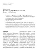
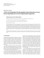
Figure 1: Deviation distributions with feature selection (solid line)
and without feature selection (dashed line). The x-axis denotes the
deviation, namely, the difference of the estimated error and the true
error; the y-axis corresponds to the density.
The most obvious is its accuracy, and this is most directly an-
alyzed via the deviation distribution of the estimator, that is,
the distribution of the difference between the estimated and
true errors. Model-based simulation studies indicate that,
given a prior set of features, cross-validation does not per-

form as well in this regard as bootstr ap or bolstered esti-
mators [2, 3]. Model-based simulation also indicates that,
given a prior set of features, cross-validation does not per-
form well when ranking feature sets of a given size [4]. More-
over, when doing feature selection, similar studies show that
cross-validation does not do well in comparison to bootst rap
and bolstered estimators when used inside forward search al-
gorithms, such as sequential forward selection and sequential
forward floating selection [5].
Here we are concerned with the use of cross-validation to
estimate the error of a classifier designed in conjunction with
feature selection. This issue is problematic because, owing
to the computational burden of bootstrap and the analytic
formulation of bolstering, these are not readily amenable to
situations where there are thousands of features from which
to choose. As in the case of prior-chosen features, the main
concern here is the deviation distribution between the cross-
validation error estimates and the true errors of the de-
signed classifiers. Owing to the added complexity of feature
selection, one might surmise that the situation here would
be worse than that for a given feature set, and it is. Even
with a given feature set, the deviation distribution for cross-
validation tends to have high variance, which is why its per-
formance genera lly is not good, especially for leave-one-out
cross-validation [2]. We observe in the current study that the
cross-validation deviation distribution is significantly flat-
ter when there is feature selection, which means that cross-
validation estimates are even more unreliable than for given
feature sets, and that they are sufficiently unreliable to raise
serious concerns when such estimates are reported. Figure 1

shows the typical deviation distributions of cross-validation
(i) with feature selection (solid line) and (ii) w ithout feature
selection, that is, using the known best features (dashed line).
In the simulations to be performed, we choose the models
such that the optimal feature set is directly obtainable from
the model, and an existing test bed provides the best feature
sets for the patient data.
A study comparing several resampling error-estimation
methods has recently addressed the inaccuracy of cross-
validation in the presence of feature selection [6]. Using
four classification rules (linear discriminant analysis, diago-
nal discriminant analysis, nearest neighbor, and CART), the
study compares bias, standard deviation, and mean-squared
error. Both simulated and patient data are used, and the t-
test is employed for feature selection. Our work differs from
[6] in two substantive ways. The major difference is that we
employ a comparative quantitative methodology by studying
the deviation distributions and defining a measure that iso-
lates as well as assesses the effects of feature selection on the
deviation analysis of cross-validation. This is necessary in or-
der to quantify the contribution of feature selection in its role
as part of the classification rule. This quantitative approach
shows that the negative effects of feature selection depend
very much on the underlying classification rule. A second
difference is that our study uses three different algorithms,
namely, t-test, sequential forward selection (SFS), and the se-
quential forward floating selection (SFFS) algorithm [7]to
select features, whereas [6] relies solely on t-test feature se-
lection. The cost for using SFS and SFFS in a large simulation
study is that they are heavily computational and therefore

we rely on high-performance computing using a Beowulf
cluster.
A preliminar y report on our study was presented at the
IEEE International Workshop on Genomic Signal Processing
and Statistics for 2006 [8].
2. SYSTEMS AND METHODS
Our interest is with the deviation distribution of an error es-
timator, that is being the distribution of difference between
the estimated and true errors of a classifier. Three classifi-
cation rules will be considered: linear discriminant analysis
(LDA), 3-nearest-neighbor (3NN), and linear support vec-
tor machine (SVM). Our method is to compare the cross-
validation (k-fold and leave-one-out) deviation distributions
for classification rules used with and without feature selec-
tion. For feature selection, we will consider three algorithms:
t-test, SFS, and SFFS (see Appendix A). Doing so will allow us
to evaluate the degree of deterioration in deviation variance
resulting from feature selection. In the case without feature
selection, the known best d features among the full feature
set will be applied for classification. It is expected that fea-
ture selection will result in a larger deviation variance than
without feature selection, which is confirmed in this study.
2.1. Coefficient of relative increase
in deviation dispersion
Given a sample set S, we use the following notations for clas-
sification errors. For the exact mathematical formulae of the
cross-validation errors, please refer to Appendix B.
Yufei Xiao et al. 3
(E) The true error of a classifier in the presence of fea-
ture selection, obtained by performing feature selec-

tion and designing a classifier on S, and then find-
ing the classification error on a large independent test
sample S

.
(E
b
) The true error of a classifier using the known best fea-
tures, obtained by designing a classifier on S with the
known best feature set, and then finding the classifica-
tion error on a large independent test sample S

.
(

E) The (k-fold or leave-one-out) cross-validation error
in the presence of feature selection. To obtain the k-
fold cross-validation error: divide the sample data into
k portions as evenly as possible. During each fold of
cross-validation, use one portion as the test sample
and the rest as the training sample; perform feature se-
lection and design a classifier on the training sample,
and estimate its error on the test sample. Find the av-
erage error of k-folds, which is

E. Leave-one-out error
is a special case when k equals the sample size.
(

E

b
) The (k-fold or leave-one-out) cross-validation error
with the best features, obtained by performing cross-
validation using the known best features.
Based on these errors, we are interested in the following
deviations, referring to the difference of the estimated error
and the true error:
(ΔE)definedas

E − E;
(ΔE
b
)definedas

E
b
− E
b
.
To quantify the effect of feature selection on cross-vali-
dation variance, using the deviation variances we define the
coefficient of relative increase in deviation dispersion (CRIDD)
by
κ
=
Var(ΔE) − Var

ΔE
b


Var(ΔE)
. (1)
Notice that κ is a relative measure, which is normalized
by Var(ΔE), because we are concerned with the relative
change of deviation variance in the presence of feature selec-
tion. In our experiments, κ is expected to be positive, because
ΔE contains two sources of uncertainty: cross-validation and
feature selection, while ΔE
b
contains none of the latter. When
positive, κ will be in the range of (0, 1], which indicates a de-
terioration in the deviation variance, due to the difference of
with and without feature selection, and the larger κ is, the
more severe the impact of feature selection.
2.2. Data
The models for simulated data take into account two require-
ments. First, in genomic applications, classification usually
involves a large number of correlated features and the sam-
ple size is out-numbered by the features; and second, we
need to know from the model the best feature set. We con-
sider the following three models under the assumption of
two equiprobable classes (classes 0 and 1).
(a) Equal covariance model: the classes 0 and 1 are drawn
from multivariate Gaussian distributions (µ
a
, Σ)and
200180160140120100806040200
0
0.05
0.1

0.15
0.2
0.25
0.3
0.35
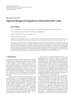
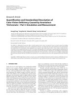
Figure 2: Vector µ = (μ
1
, μ
2
, , μ
200
). The x-axis denotes μ
1
,
μ
2
, , μ
200
, and the y-axisdenotestheirvalues.
(−µ
a
, Σ), respectively, the optimal classifier on the full
feature-label distribution being given by LDA.
(b) Unequal covariance model: the classes 0 and 1
are drawn from multivariate Gaussian distributions
(µ
b
, Σ)and(−µ
b
,2Σ), respectively, the optimal classi-

fier on the full feature-label distribution being given by
quadratic discriminant analysis (QDA).
(c) Bimodal model: class 0 is generated from a multivari-
ate Gaussian distribution (0, Σ) and class 1 is gener-
ated from a mixture of two equiprobable multivariate
Gaussian distributions (µ
c
, Σ)and(−µ
c
, Σ).
For the above models, we have chosen µ
a
=µ
b
=1.75µ and
µ
c
= 4.0µ,whereµ = (μ
1
, , μ
200
) is plotted in Figure 2 (for
details of generating µ, please go to the companion website
/>fscv/generate mu.pdf).
Notice that the scaling factors (1.75 and 4.0) control how far
apart the class 0 and class 1 data are, such that classification is
possible but not too easy. It can be seen from the figure that
μ
1
, μ

21
, μ
41
, , μ
181
are much larger in magnitude than the
others. The covariance matrix Σ has a block-diagonal struc-
ture, with block size 20. In each of the 10 diagonal blocks,
the elements on the main diagonal are 1.0, while all others
are equal to ρ. In all of the simulated data experiments, we
choose ρ
= 0.1. Therefore, among the 200 features, the best
10 features are the 1st, 21st, , 181st features, which are
mutually independent. Each of the best 10 features is weakly
correlated with 19 other nonbest features (ρ
= 0.1).
The experiments on simulated data are designed for two
different sizes of sample S, N
= 50 and N = 100. The size
of the independent test data set S

for getting true error is
5000. Each data point is a random vector with dimensionality
200, and 10 features will be selected by the feature selection
algorithm. In all the three models, the numbers of sample
points from class 0 and class 1 are equal (N/2).
The patient data come from 295 breast tumor microar-
rays, each obtained from one patient [9, 10] and together
yielding 295 log-expression profiles. Based on patient sur-
vival data and other clinical measures, 180 data points fall

into the “good prognosis” class and 115 fall into the “bad
4 EURASIP Journal on Bioinformatics and Systems Biology
prognosis” class, the two classes to be labeled 0 and 1, respec-
tively. Each data point is a 70-gene expression vector. The 295
70-expression vectors constitute the empirical sample space,
with prior probabilities about 0.6 and 0.4, respectively. For
error e stimation, we will randomly draw a stratified sample
of size 35 (i.e., S) from the 295 data points, without replace-
ment. In the sample, 21 data points belong to class 0, and 14
belong to class 1. From the full set of 70 genes, 7 w ill be se-
lected for classification, where both k-fold (k
= 7) and leave-
one-out cross-validation will be used for error estimation.
The key reason for using this data set is that it is incorporated
into a feature-set test bed and the 7 best genes are known for
3NN and LDA, these having been derived from a full search
among all possible 7-gene feature sets from the full 70 genes
[11]. Since the SVM optimal genes are not derived in the test
bed, we will use the LDA best genes to obtain the distribution
of ΔE
b
. To obtain the true classification error, the remaining
260
= 295 − 35 data points will constitute S

and be tested
on. Since the size of S is small, compared to the full dataset
of 295, the dependence between t wo random samples will be
negligible (see [2] for an analysis of the dependency issue in
the context of this data set).

3. IMPLEMENTATION
We consider three commonly employed classification rules:
LDA, 3NN, and SVM. All three are used on all data mod-
els, with the exception that only 3NN is applicable to the bi-
modal model. As stated previously, our method is to com-
pare the cross-validation (k-fold and leave-one-out) devia-
tion distributions for classification rules used with and with-
out feature selection. For feature selection, we use t-test, SFS,
and SFFS to select d features from the full feature set. To im-
prove feature selection accuracy, within SFS and SFFS, the
feature selection criterion is semibolstered resubstitution er-
ror with 3NN classifier, or bolstered resubstitution error with
LDA and SVM classifiers [5].
To accomplish our goal, we propose the following experi-
ments on simulated and patient data. Draw a random sample
S of size N from the sample space, select d features on S,and
denote the feature set by F. Design a classifier C
F
on S,and
test it on a large independent sample S

to get the true error
E. Design a classifier C
b
on S with the known best feature
set F
b
, and find the true error E
b
by testing it on S


.Obtain
the (k-fold or leave-one-out) cross-validation errors

E and

E
b
.ComputeΔE =

E − E and ΔE
b
=

E
b
− E
b
. Finally, repeat
the previous sampling and error estimation procedure 10000
times, and plot the empirical distributions of ΔE and ΔE
b
.
A step-by-step description that provides the implemen-
tation of proposed experiments is shown in Algorithm 1.
We use abbreviations CV and LOO for cross-validation and
leave-one-out, respectively.
4. RESULTS AND DISCUSSION
Let us first consider the simulated data. Three classifiers,
LDA, 3NN, and SVM, are applied to the simulated data with

sample sizes N
= 50 and N = 100, and all three model
distributions, with the exception that only 3NN is appli-
cable to the bimodal model. Three feature selection algo-
rithms, t-test, SFS, and SFFS, are employed, with the ex-
ception that only SFS and SFFS are applicable to the bi-
modal model. In each case, two kinds of cross-validation er-
ror estimation methods, 10-fold cross-validation (CV10) and
leave-one-out (LOO), are used. The complete plots of devi-
ation distributions are provided on the companion website
( />fscv/). Here, Figure 3
shows the deviation distributions for the unequal covariance
model using CV10. The plots in Figure 3 are fairly typical.
Table s 1, 2,and3 list the deviation variances and κ for ev-
ery model, classifier, and feature selection algorithm. From
the tables, we observe that κ is always positive, confirm-
ing that feature selection worsens error estimation precision.
Please note that since no feature selection is involved in ob-
taining E
b
and

E
b
, ΔE
b
is independent of feature selection
methods. Therefore, in each row of the tables (with fi xed clas-
sifier and cross-validation method), we combine the ΔE
b

’s of
the three experiments (t-test, SFS, and SFFS) and compute
the overall variance Var(ΔE
b
)(pooledvariance).
When interpreting the results, two related issues need to
be kept in mind. First, we are interested in measuring the
degree to which feature selection degrades cross-validation
performance for different feature selection methods, not the
performance of the feature selection methods themselves. In
particular, two studies have demonstrated the performance
of SFFS [12, 13], and for the linear model with weak cor-
relation we can expect good results from the t-test. Second,
since the performance of an error estimator depends on its
bias and variance, when choosing between feature selection
algorithms we prefer a smaller deviation variance Var(ΔE).
The results show that a smaller variance of ΔE usually corre-
sponds to a smaller κ, but not strictly so, because κ depends
on the variance of ΔE
b
too. For instance, with the equal co-
variance model and t-test, when the sample size is 50 and
10-fold CV is used, the 3NN classifier gives a smaller vari-
ance of ΔE than the SVM classifier, whereas its κ is larger
than SVM. Be that as it may, the sole point of this study is to
quantify the increase in variance owing to feature selection,
thereby characterizing the manner in which feature selection
impacts upon cross-validation error estimation for combina-
tions of feature selection algorithms and classification rules.
Looking at the results, we see that the degradation in de-

viation variance owing to feature selection can be striking,
especially in the bimodal model, where κ exceeds 0.81 for all
cases in Table 3. In the unequal covariance model, for sample
size 50, κ generally exceeds 0.45. One can observe differences
in the effects of feature selection relative to the classification
rule and feature selection algorithm by perusing the tables.
An interesting phenomenon to observe is the effect of in-
creasing the sample size from 50 to 100. In all cases, this sig-
nificantly reduces the variances, as expected; however, while
increased sample size reduces κ for the t-test, there is no sim-
ilar reduction observed for SFS and SFFS with the unequal
covariance model. Perhaps here it would be beneficial to em-
phasize that the performance of the t-test on the simulated
data may be due to the nature of the equal covariance and
Yufei Xiao et al. 5
(1) Specify the following parameters:
N
MC
= 10000; /∗ number of Monte Carlo experiments∗/
d;/
∗number of features to be selected∗/
N
sample
;/∗sample size∗/
N
fold
;/∗=k if k-fold CV; = N
sample
if LOO∗/
best feature set F

b
;/∗containing d best features; ∗/
(2) n
MC
= 0; /∗loop count∗/
(3) while ( n
MC
<N
MC
) {
(a) Generate a random sample S of size N
sample
from the sample space, with N
sample
∗p
0
data points f rom class 0, and N
sample
∗p
1
data points from class 1, where p
0
and p
1
are the prior probabilities.
(b) Use the best feature set F
b
to design a classifier C
b
on S. Perform feature selection on S to obtain a feature set F of d

features. Use F to design a classifier C
F
on S.
(c) To obtain the true classification errors, generate a large sample S

independent of S to test C
F
and C
b
, then denote their
true errors by E and E
b
,respectively.
(d) To do N
fold
-fold cross-validation, divide the data evenly into N
fold
portions T
0
, , T
N
fold
−1
, and in each portion, the num-
bers of class 0 data and class 1 data are roughly proportional to p
0
and p
1
, if possible.
(e) For (i

= 0; i<N
fold
; i ++){
(i) Hold out T
i
as the test sample and use S \ T
i
as the t raining sample.
(ii) Perform feature selection on the training sample, and the resultant feature set is F
i
of size d.
(iii) Apply feature set F
i
, and use the training sample to desig n a surrogate classifier C
i
,andtestC
i
on T
i
to obtain the
estimated error

E
i
.
(iv) Repeat step (iii), but use feature set F
b
instead, to obtain the surrogate classifier C
b,i
and error


E
b,i
.
}
(f) Find the average errors

E and

E
b
over the N
fold
folds.
(g) Compute the differences between the estimated and the true errors,
ΔE
=

E − E,
ΔE
b
=

E
b
− E
b
.
(h) n
MC

++.
}
(4) From the N
MC
Monte Carlo experiments, plot the empirical distributions of ΔE and ΔE
b
,respectively.
Algorithm 1: Simulation scheme
Table 1: Results for simulated data: equal covariance model. For easy reading, the variances are in 10
−4
unit.
N Classifier
t-test SFS SFFS
Var(ΔE)Var(ΔE
b
) κ Var(ΔE)Var(ΔE
b
) κ Var(ΔE)Var(ΔE
b
) κ
50
3NN,CV10 25.76 16.48 0.3605 62.79 16.48 0.7376 62.26 16.48 0.7354
3NN,LOO 26.11 17.05 0.3469 65.05 17.05 0.7378 63.05 17.05 0.7295
LDA,CV10 32.21 17.48 0.4572 50.84 17.48 0.6561 51.76 17.48 0.6622
LDA,LOO 30.00 16.35 0.4552 52.59 16.35 0.6892 56.79 16.35 0.7121
SVM,CV10 35.89 25.21 0.2976 54.76 25.21 0.5397 52.47 25.21 0.5195
SVM,LOO 38.35 26.38 0.3121 51.81 26.38 0.4908 53.71 26.38 0.5088
100
3NN,CV10 7.96 7.42 0.0677 25.53 7.42 0.7094 25.12 7.42 0.7046
3NN,LOO 7.53 7.38 0.0197 24.55 7.38 0.6993 24.24 7.38 0.6954

LDA,CV10 6.55 6.00 0.0841 13.18 6.00 0.5448 13.04 6.00 0.5400
LDA,LOO 6.18 5.74 0.0716 12.90 5.74 0.5555 13.79 5.74 0.5840
SVM,CV10 10.29 9.74 0.0538 17.16 9.74 0.4326 16.79 9.74 0.4201
SVM,LOO 11.20 10.52 0.0611 16.20 10.52 0.3508 15.79 10.52 0.3338
6 EURASIP Journal on Bioinformatics and Systems Biology
0.50−0.5
0
2
4
6
8
(a) 3NN + t-test
0.50−0.5
0
2
4
6
8
(b) 3NN + SFS
0.50−0.5
0
2
4
6
8
(c) 3NN + SFFS
0.50−0.5
0
2
4

6
8
(d) LDA + t-test
0.50−0.5
0
2
4
6
8
(e) LDA + SFS
0.50−0.5
0
2
4
6
8
(f) LDA + SFFS
0.50−0.5
0
2
4
6
8
(g) SVM + t-test
0.50−0.5
0
2
4
6
8

(h) SVM + SFS
0.50−0.5
0
2
4
6
8
(i) SVM + SFFS
Figure 3: Deviation distributions with feature selection (solid line) and without feature selection (dashed line), unequal covariance model,
10-fold CV with sample size N
= 50. The x-axis denotes the deviation, and the y-axis corresponds to the density.
Table 2: Results for simulated data: unequal covariance model. For easy reading, the variances are in 10
−4
unit.
N Classifier
t-test SFS SFFS
Var(ΔE)Var(ΔE
b
) κ Var(ΔE)Var(ΔE
b
) κ Var(ΔE)Var(ΔE
b
) κ
50
3NN,CV10 41.91 25.61 0.3890 50.24 25.61 0.4904 52.25 25.61 0.5100
3NN,LOO 46.17 25.69 0.4436 51.93 25.69 0.5054 53.10 25.69 0.5163
LDA,CV10 57.85 27.16 0.5304 66.44 27.16 0.5912 68.21 27.16 0.6018
LDA,LOO 61.85 25.33 0.5905 74.46 25.33 0.6598 82.06 25.33 0.6913
SVM,CV10 60.05 34.85 0.4197 68.71 34.85 0.4929 68.27 34.85 0.4896
SVM,LOO 70.06 37.23 0.4685 68.67 37.23 0.4578 69.81 37.23 0.4666

100
3NN,CV10 13.75 11.60 0.1562 29.17 11.60 0.6022 28.98 11.60 0.5996
3NN,LOO 13.97 11.79 0.1560 27.42 11.79 0.5699 28.37 11.79 0.5843
LDA,CV10 12.67 9.92 0.2170 22.42 9.92 0.5576 22.39 9.92 0.5570
LDA,LOO 12.77 9.51 0.2556 23.99 9.51 0.6038 25.42 9.51 0.6260
SVM,CV10 16.88 13.81 0.1816 25.85 13.81 0.4657 25.14 13.81 0.4506
SVM,LOO 18.74 15.19 0.1895 24.44 15.19 0.3786 23.09 15.19 0.3422
Yufei Xiao et al. 7
Table 3: Results for simulated data: bimodal model. For easy reading, the variances are in 10
−4
unit.
Sample
size N
Classifier
SFS SFFS
Var(ΔE)Var(ΔE
b
) κ Var(ΔE)Var(ΔE
b
) κ
50
3NN,CV10 134.80 15.91 0.8820 141.94 15.91 0.8879
3NN,LOO 116.54 15.72 0.8651 126.08 15.72 0.8754
100
3NN,CV10 47.07 6.77 0.8562 40.94 6.77 0.8346
3NN,LOO 39.21 6.74 0.8280 36.55 6.74 0.8155
0.50−0.5
0
1
2

3
4
5
6
(a) 3NN + t-test
0.50−0.5
0
1
2
3
4
5
6
(b) 3NN + SFS
0.50−0.5
0
1
2
3
4
5
6
(c) 3NN + SFFS
0.50−0.5
0
1
2
3
4
5

6
(d) LDA + t-test
0.50−0.5
0
1
2
3
4
5
6
(e) LDA + SFS
0.50−0.5
0
1
2
3
4
5
6
(f) LDA + SFFS
0.50−0.5
0
1
2
3
4
5
6
(g) SVM + t-test
0.50−0.5

0
1
2
3
4
5
6
(h) SVM + SFS
0.50−0.5
0
1
2
3
4
5
6
(i) SVM + SFFS
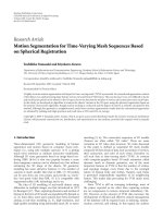
Figure 4: Deviation distributions with feature selection (solid line) and without feature selection (dashed line) for patient data, 7-fold CV.
The x-axis denotes the deviation, and the y-axis corresponds to the density.
unequal covariance models: specifically, to obtain the devia-
tion distribution without feature selection, we have to know
the optimal feature set from the model, and thus we have
chosen the features to be either uncorrelated or weakly cor-
related, a setting, that is, advantageous for the t-test.
When turning to the patient data (see Table 4, and the
pooled variances are used, like in the previous three tables),
one is at once struck by the fact that κ is quite consistent
across the three-feature selection methods. It differs accord-
ing to the classification rule and cross-validation procedure,
being over 0.4 for all feature selection methods with LDA and

LOO, and being below 0.13 for all methods with SVM and
LOO; however, the changes b etween feature selec tion meth-
ods for a given classification rule and cross-validation proce-
dureareverysmall,asshownclearlyinFigure 4. This con-
sistency results in part from the fact that, with the patient
8 EURASIP Journal on Bioinformatics and Systems Biology
Table 4: Results for patient data. For easy reading, the variances are in 10
−4
unit.
Classifier
t-test SFS SFFS
Var(ΔE)Var(ΔE
b
) κ Var(ΔE)Var(ΔE
b
) κ Var(ΔE)Var(ΔE
b
) κ
3NN,CV7 77.10 54.74 0.2900 83.88 54.74 0.3474 83.62 54.74 0.3454
3NN,LOO
90.24 56.27 0.3764 93.05 56.27 0.3953 93.39 56.27 0.3975
LDA,CV7 84.85 60.89 0.2824 85.72 60.89 0.2896 86.05 60.89 0.2923
LDA,LOO
99.49 56.98 0.4273 96.89 56.98 0.4120 95.82 56.98 0.4054
SVM,CV7 74.75 57.92 0.2252 78.47 57.92 0.2620 78.12 57.92 0.2586
SVM,LOO
96.10 84.45 0.1212 94.92 84.45 0.1103 95.04 84.45 0.1114
Table 5: Squared biases for simulated data: equal covariance model. The squared biases are in 10
−4
unit, the same as deviation variances.

N Classifier
t-test SFS SFFS
Mean
2
(ΔE) Mean
2
(ΔE
b
) Mean
2
(ΔE) Mean
2
(ΔE
b
) Mean
2
(ΔE) Mean
2
(ΔE
b
)
50
3NN,CV10 0.58 0.03 1.72 0.03 1.91 0.03
3NN,LOO 0.33 0.14 0.73 0.14 0.74 0.14
LDA,CV10 1.24 0.14 2.10 0.14 2.17 0.14
LDA,LOO 0.13 0.01 0.13 0.01 0.21 0.01
SVM,CV10 1.02 0.10 2.19 0.10 1.78 0.10
SVM,LOO 0.22 0.06 0.47 0.06 0.52 0.06
100
3NN,CV10 0.03 0.01 0.82 0.01 0.69 0.01

3NN,LOO 0.01 0.01 0.12 0.01 0.12 0.01
LDA,CV10 0.07 0.02 0.47 0.02 0.42 0.02
LDA,LOO 0.00 0.00 0.00 0.00 0.01 0.00
SVM,CV10 0.11 0.04 0.47 0.04 0.51 0.04
SVM,LOO 0.00 0.00 0.08 0.00 0.06 0.00
data, we are concerned with a single feature-label distribu-
tion. On the other hand, the consistency is also due to the
similar effects on error estimation of the different feature se-
lection methods with this feature-label distribution, a distri-
bution in which there are strong correlations among some of
the features (gene expressions).
Our interest is in quantifying the increase in variance re-
sulting from feature selection; nevertheless, since the mean-
squared error of an error estimator equals the sum of the
variance and the squared bias, one might ask whether fea-
ture selection has a significant impact on the bias. Given
that the approximate unbiasedness of cross-validation ap-
plies to the classification rule a nd that feature selection is
part of the classification rule, we would not expect a sig-
nificant effect on the bias. This expectation is supported by
the curves in the figures, since the means of the with- and
without-feature-selection deviation curves tend to be close.
We should, however, not expect these means to be identical,
because the exact manner in w hich the expectation of the er-
ror estimate approximates the true error depends upon the
classification rule and sample size. To be precise, for k-fold
cross-validation with feature selection, the bias is given by
Bias
FS(D,d)
N,k

= E

ε
FS(D,d)
N
−N/k

−
E

ε
FS(D,d)
N

,(2)
where ε
FS(D,d)
N,k
denotes the error for the classification rule
when incorporating feature selection to choose d from
among D features based on a sample size of N. Without fea-
ture selection, the bias is given by
Bias
(d)
N,k
= E

ε
(d)
N

−N/k

−
E

ε
(d)
N

,(3)
where ε
(d)
N,k
denotes the error for the classification r ule with-
out feature selection using d features based on a sample size
of N. The bias (difference in expectation) depends upon the
classification rule, including whether or not feature selection
is employed.
To quantify the effect of feature selection on bias, we
have computed the squared biases of the estimated errors,
both with and without feature selection (namely, the squared
means of ΔE and ΔE
b
), for the cases considered. Squared bi-
ases are computed because the y appear in the mean-squared
errors. These are given in Tables 5, 6, 7,and8, corresponding
to Tables 1, 2, 3,and4, respectively. For the model-based data
from the equal and unequal covariance models, we see in Ta-
bles 5 and 6 that the bias tends to be a bit larger w ith feature
selection, but the squared bias is still negligible in compar-

ison to the variance, the squared biases tending to be very
small when N
= 100. A partial exception occurs for the bi-
modal model when there is feature selection. In Table 7,we
see that, for SFS and SFFS, mean
2
(ΔE) > 7 × 10
−4
for 3NN,
CV10, and N
= 50. Even here, the squared biases are small
Yufei Xiao et al. 9
Table 6: Squared biases for simulated data: unequal covariance model. The squared biases are in 10
−4
unit, the same as dev i ation variances.
N Classifier
t-test SFS SFFS
Mean
2
(ΔE) Mean
2
(ΔE
b
) Mean
2
(ΔE) Mean
2
(ΔE
b
) Mean

2
(ΔE) Mean
2
(ΔE
b
)
50
3NN,CV10 1.58 0.19 0.99 0.19 1.02 0.19
3NN,LOO 0.81 0.33 0.69 0.33 0.83 0.33
LDA,CV10 2.81 0.21 2.29 0.21 2.96 0.21
LDA,LOO 0.19 0.02 0.22 0.02 0.35 0.02
SVM,CV10 2.29 0.20 2.77 0.20 1.96 0.20
SVM,LOO 0.56 0.07 0.87 0.07 0.99 0.07
100
3NN,CV10 0.35 0.05 0.88 0.05 1.02 0.05
3NN,LOO 0.07 0.04 0.08 0.04 0.21 0.04
LDA,CV10 0.31 0.04 0.91 0.04 0.82 0.04
LDA,LOO 0.00 0.00 0.04 0.00 0.02 0.00
SVM,CV10 0.48 0.07 0.91 0.07 0.85 0.07
SVM,LOO 0.02 0.02 0.07 0.02 0.05 0.02
Table 7: Squared biases for simulated data: bimodal model. The squared biases are in 10
−4
unit, the same as deviation variances.
Sample
size N
Classifier
SFS SFFS
Mean
2
(ΔE) Mean

2
(ΔE
b
) Mean
2
(ΔE) Mean
2
(ΔE
b
)
50
3NN,CV10 7.27 0.10 8.31 0.10
3NN,LOO 1.68 0.12 2.36 0.12
100
3NN,CV10 3.24 0.02 2.26 0.02
3NN,LOO 0.32 0.02 0.06 0.02
in comparison to the corresponding variances, where we see
in Table 3 that Var(ΔE) > 134
× 10
−4
for both SFS and SFFS.
Finally, we note that for the patient data in Table 8 we ha v e
omittedSVMbecausewehaveusedtheLDAoptimalfeatures
from the test bed and therefore the relationship between the
bias with and without feature selection is not directly inter-
pretable.
5. CONCLUSION
We have introduced the coefficient of relative increase in de-
viation dispersion to quantify the effect of feature selection
on cross-validation error estimation. The coefficient mea-

sures the relative increase in the variance of the deviation
distribution due to feature selection. We have computed the
coefficient for the LDA, 3NN, and linear SVM classifica-
tion rules, using three feature selection algorithms, t-test,
SFS, and SFFS, and two cross-validation methods, k-fold
and leave-one-out. We have applied the coefficient to several
feature-label models and patient data from a breast cancer
study. The models have been chosen so that the optimal fea-
ture set is directly obtainable from the model and the feature-
selection test bed provides the best feature sets for the patient
data.
Any factor that can influence error estimation and fea-
ture selection can influence the CRIDD, and these are nu-
merous: the classification rule, the feature-selection algo-
rithm, the cross-validation procedure, the feature-label dis-
tribution, the total number of potential features, the number
of useful features among the total number available, the prior
class probabilities, and the sample size. Moreover, as is typi-
cal in classification, there is interaction among these factors.
Our purpose in this paper has been to introduce the CRIDD
and, to this end, we have examined a number of combina-
tions of these factors using both model and patient data in
order to illustrate how the CRIDD can be utilized in partic-
ular situations. Assuming one could overcome the computa-
tional impediment, an objective of future work would be to
carry out a rigorous study of the factors affecting the man-
ner in which feature-selection impacts cross-validation error
estimation, perhaps via an analysis-of-variance approach ap-
plied to the factors affecting the CRIDD.
This having been said, we would like to specifically com-

ment on two issues for future study. The first concerns the
modest feature-set sizes considered in this study relative to
the number of potential features often encountered in prac-
tice, such as the thousands of genes on an expression mi-
croarray. The reason for choosing the feature-set sizes used
in the present paper is because of the extremely long compu-
tation times involved in a general study. Even using our Be-
owulf cluster, computation time is prohibitive when so many
cases are being studied. It is reasonable to conjecture that
the increased cross-validation variance owing to feature se-
lection that we have observed will hold, or increase, when
larger numbers of potential features are observed; however,
the exact manner in which this occurs will depend on the
10 EURASIP Journal on Bioinformatics and Systems Biology
Table 8: Squared biases for patient data. The squared biases are in 10
−4
unit, the same as deviation variances.
Classifier
t-test SFS SFFS
Mean
2
(ΔE) Mean
2
(ΔE
b
) Mean
2
(ΔE) Mean
2
(ΔE

b
) Mean
2
(ΔE) Mean
2
(ΔE
b
)
3NN,CV7 0.08 0.19 0.39 0.19 0.34 0.19
3NN,LOO
1.78 0.81 1.10 0.81 1.28 0.81
LDA,CV7 0.47 0.53 0.52 0.53 0.77 0.53
LDA,LOO
0.17 0.04 0.34 0.04 0.08 0.04
proportion of useful features among the potential features
and the nature of the feature-label distributions involved.
Owing to computational issues, one might have to be con-
tented with considering special cases of interest, rather than
looking across a wide spectrum of conditions. As a counter-
point to this cautionary note, one needs only to recognize the
recent extraordinary expansion of computational capability
in bioinformatics.
A second issue concerns the prior probabilities of the
classes. In this study (and common among many classifica-
tion studies), for both synthetic and patient data, the classes
are either equiprobable or close to equiprobable. In the case
of small samples, when the prior probabilities are substan-
tially unbalanced, feature selection b ecomes much harder,
and we expect that variation in error estimation will grow
and this will be reflected in a larger CRIDD. There are two

codicils to this point: (1) the exact nature of the unbalanced
effect will depend on the feature-label distributions, feature-
selection algorithm, and the other remaining factors, and (2)
when there is severe lack of balance between the classes, the
overall classification error rate may not be a good way to
measure prac tical classification performance—for instance,
with extreme unbalance, good classification results from sim-
ply choosing the value of the dominant class no matter the
observation—and hence the whole approach discussed in
this study may not be appropriate.
APPENDICES
A. FEATURE SELECTION METHODS: SFS AND SFFS
A common approach to suboptimal feature selection is se-
quential selection, either forward or backward, and their
variants. Sequential forward select ion (SFS) begins with a
small set of features, perhaps one, and iteratively builds
the feature set. When there are k features, x
1
, x
2
, , x
k
,
in the growing feature set, all feature sets of the form
{x
1
, x
2
, , x
k

, w} are compared and the best one is chosen to
form the feature set of size k + 1. A problem with SFS is that
there is no way to delete a feature adjoined early in the iter-
ation that may not perform as well in combination as other
features. The SFS look-back algorithm aims to mitigate this
problem by allowing deletion. For it, when there are k fea-
tures, x
1
, x
2
, , x
k
,inthegrowingfeatureset,allfeaturesets
of the form
{x
1
, x
2
, , x
k
, w, z} are compared and the best
one is chosen. Then all (k + 1)-element subsets are checked
to allow the possibility of one of the earlier chosen features
to be deleted, the result being the k + 1 features that will
form the basis for the next stage of the algorithm. Flexibility
is added with the sequential forward floating selection (SFFS)
algorithm, where the number of features to be adjoined and
deleted is not fixed [7]. Simulation studies support the effec-
tiveness of SFFS [12, 13]; however, with small samples SFFS
performance is significantly affected by the choice of error

estimator used in the selection process, with bolstered error
estimators giving comparatively good results [5].
B. CROSS-VALIDATION ERROR
In two-group statistical pattern recognition, there is a fea-
ture vector X
∈ R
p
and a label Y ∈{0, 1}. The joint
probability distribution F of (X, Y ) is unknown in prac-
tice. Hence, one has to design classifiers from training data,
which consists of a set of n independent observations, S
n
=
{
(X
1
, Y
1
), ,(X
n
, Y
n
)},drawnfromF.Aclassification rule is
a mapping g :
{R
p
×{0, 1}}
n
× R
p

→{0, 1}. A classifica-
tion rule maps the training data S
n
into the designed classifier
g(S
n
, ·):R
p
→{0, 1}.Thetrue error of a designed classifier
is its error rate given the training data set

n

g | S
n

= P

g

S
n
, X

/= Y

= E
F




Y − g

S
n
, X




,
(B.1)
where the notation E
F
indicates that the expectation is taken
with respect to F; in fact, one can think of (X, Y) in the above
equation as a random test point (this interpretation being
useful in understanding error estimation). The expected er-
ror rate over the data is given by

n
[g] = E
F
n


n

g | S
n


= E
F
n
E
F



Y − g

S
n
, X




,
(B.2)
where F
n
is the joint distribution of the training data S
n
. This
is sometimes called the unconditional error of the classifica-
tion rule, for sample size n.
In k-fold cross-validation, the data set S
n
is partitioned

into k folds S
(i)
,fori = 1, , k (for simplicity, we assume
that k divides n). Each fold is left out of the design process
and used as a test set, and the estimate is the overall propor-
tion of error committed on all folds:


cvk
=
1
n
k

i=1
n/k

j=1


y
(i)
j
− g

S
n
\ S
(i)
, x

(i)
j



,(B.3)
where (x
(i)
j
, y
(i)
j
) is a sample in the ith fold. The process
may be repeated: several cross-validation estimates are com-
puted using different partitions of the data into folds, and
Yufei Xiao et al. 11
the results are averaged. A k-fold cross-validation estima-
tor is unbiased as an estimator of

n−n/k
[g]. The most well-
known cross-validation method is the leave-one-out estima-
tor, whereby a s ingle observation is left out each time:


loo
=
1
n
n


i=1


y
i
− g

S
i
n
−1
, x
i



,(B.4)
where S
i
n
−1
is the data set resulting from deleting data point
i from the original data set S
n
. This corresponds to n-fold
cross-validation.
ACKNOWLEDGMENT
This research has been supported in part by the National Sci-
ence Foundation, Grants CCF-0514644 and BES-0536679.

REFERENCES
[1] L.Devroye,L.Gyorfi,andG.Lugosi,A Probabilistic Theor y of
Pattern Recognition, Springer, New York, NY, USA, 1996.
[2] U. Braga-Neto and E. R. Dougherty, “Is cross-validation valid
for small-sample microarray classification?” Bioinformatics,
vol. 20, no. 3, pp. 374–380, 2004.
[3] U. Braga-Neto and E. R. Dougherty, “Bolstered error estima-
tion,” Pattern Recognition, vol. 37, no. 6, pp. 1267–1281, 2004.
[4] C. Sima, U. Braga-Neto, and E. R. Dougherty, “Superior
feature-set ranking for s mall samples using bolstered error es-
timation,” Bioinformatics, vol. 21, no. 7, pp. 1046–1054, 2005.
[5] C.Sima,S.Attoor,U.Brag-Neto,J.Lowey,E.Suh,andE.R.
Dougherty, “Impact of error estimation on feature selection,”
Pattern Recognition, vol. 38, no. 12, pp. 2472–2482, 2005.
[6] A. M. Molinaro, R. Simon, and R. M. Pfeiffer, “Prediction er-
ror estimation: a comparison of resampling methods,” Bioin-
formatics, vol. 21, no. 15, pp. 3301–3307, 2005.
[7] P. Pudil, J. Novovicova, and J. Kittler, “Floating search methods
in feature selection,” Pattern Recognition Letters, vol. 15, no. 11,
pp. 1119–1125, 1994.
[8] Y. Xiao, J. Hua, and E. R. Dougherty, “Feature selection in-
creases cross-validation imprecision,” in Proceedings of the 4th
IEEE International Workshop on Genomic Signal Processing and
Statistics (GENSIPS ’06), College Station, Tex, USA, May 2006.
[9]L.J.van’tVeer,H.Dai,M.J.vandeVijver,etal.,“Geneex-
pression profiling predicts clinical outcome of breast cancer,”
Nature, vol. 415, no. 6871, pp. 530–536, 2002.
[10] M.J.vandeVijver,Y.D.He,L.J.van’tVeer,etal.,“Agene-
expression signature as a predictor of survival in breast can-
cer ,” New England Journal of Medicine, vol. 347, no. 25, pp.

1999–2009, 2002.
[11] A. Choudhary, M. Brun, J. Hua, J. Lowey, E. Suh, and E. R.
Dougher ty, “Genetic test bed for feature selection,” Bioinfor-
matics, vol. 22, no. 7, pp. 837–842, 2006.
[12] A. Jain and D. Zongker, “Feature selection: evaluation, appli-
cation, and small sample performance,” IEEE Transactions on
Pattern Analysis and Machine Intelligence, vol. 19, no. 2, pp.
153–158, 1997.
[13] M. Kudo and J. Sklansky, “Comparison of algorithms that se-
lect features for pattern classifiers,” Pattern Recognition, vol. 33,
no. 1, pp. 25–41, 2000.