Báo cáo hóa học: " Research Article Step Size Bound of the Sequential Partial Update LMS Algorithm with Periodic Input Signals" potx

Hindawi Publishing Corporation
EURASIP Journal on Audio, Speech, and Music Processing
Volume 2007, Article ID 10231, 15 pages
doi:10.1155/2007/10231
Research Article
Step Size Bound of the Sequential Partial Update LMS
Algorithm with Periodic Input Signals
Pedro Ramos,
1
Roberto Torrubia,
2
Ana L
´
opez,
1
Ana Salinas,
1
and Enrique Masgrau
2
1
Communication Technologies Group, Arag
´
on Institute for Engineering Research (I3A), EUPT, University of Zaragoza,
Ciudad Escolar s/n, 44003 Teruel, Spain
2
Communication Technologies Group, Arag
´
on Institute for Engineering Research (I3A), CPS Ada Byron, University of Zaragoza,
Maria de Luna 1, 50018 Zaragoza, Spain
Received 9 June 2006; Revised 2 October 2006; Accepted 5 October 2006
Recommended by Kutluyil Dogancay

This paper derives an upper bound for the step size of the sequential partial update (PU) LMS adaptive algorithm when the input
signal is a periodic reference consisting of several harmonics. The maximum step size is expressed in terms of the gain in step size of
the PU algorithm, defined as the ratio between the upper bounds that ensure convergence in the following two cases: firstly, when
only a subset of the weights of the filter is updated during every iteration; and secondly, when the whole filter is updated at every
cycle. Thus, this gain in step-size determines the factor by which the step size parameter can be increased in order to compensate
the inherently slower convergence rate of the sequential PU adaptive algorithm. The theoretical analysis of the strategy developed
in this paper excludes the use of certain frequencies corresponding to notches that appear in the gain in step size. This strategy
has been successfully applied in the active control of periodic disturbances consisting of several harmonics, so as to reduce the
computational complexity of the control system without either slowing down the convergence rate or increasing the residual error.
Simulated and experimental results confirm the expected behavior.
Copyright © 2007 Pedro Ramos et al. This is an open access article distributed under the Creative Commons Attribution License,
which permits unrestricted use, distribution, and reproduction in any medium, provided the original work is properly cited.
1. INTRODUCTION
1.1. Context of application: active noise
control systems
Acoustic noise reduction can be achieved by two different
methods. Passive techniques are based on the absorption and
reflection properties of materials, showing excellent noise at-
tenuation for frequencies above 1 kHz. Nevertheless, passive
sound absorbers do not work well at low frequencies be-
cause the acoustic wavelength becomes large compared to
the thickness of a typical noise barrier. On the other hand,
active noise control (ANC) techniques are based on the prin-
ciple of destructive wave interference, whereby an antinoise
is generated with the same amplitude as the undesired distur-
bance but with an appropriate phase shift in order to cancel
the pr imary noise at a given location, generating a zone of
silence around an acoustical sensor.
The basic idea behind active control was patented by
Lueg [1]. However, it was with the relatively recent advent

of powerful and inexpensive digital signal processors (DSPs)
that ANC techniques became pra ctical because of their ca-
pacity to perform the computational tasks involved in real
time.
The most popular adaptive algorithm used in DSP-based
implementations of ANC systems is the filtered-x least mean-
square (FxLMS) algorithm, originally proposed by Morgan
[2] and independently derived by Widrow et al. [3] in the
context of adaptive feedforward control and by Burgess [4]
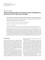
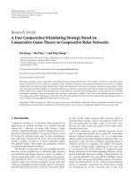
for the active control of sound in ducts. Figure 1 shows the
arrangement of electroacoustic elements and the block di-
agram of this well known solution, aimed at attenuating
acoustic noise by means of secondary sources. Due to the
presence of a secondary path transfer function following
the adaptive filter, the conventional LMS algorithm must
be modified to ensure convergence. The mentioned sec-
ondary path includes the D/A converter, power amplifier,
loudspeaker, acoustic path, error microphone, and A/D con-
verter. The solution proposed by the FxLMS is based on
the placement of an accurate estimate of the secondary path
transfer function in the weight update path as originally sug-
gested in [2]. Thus, the regressor sig nal of the adaptive filter
2 EURASIP Journal on Audio, Speech, and Music Processing
Source
of noise
Undesired noise
Error
microphone
Secondary
source

Reference
microphone
Antinoise
ANC
output
Reference
ANC
Error
y(n)
x(n) e(n)
(a)
x(n)
Reference
P(z)
Primary path
d(n)
Undesired noise
y
(n)
Antinoise
S(z)
Secondary path
y(n)
W(z)
Adaptive filter

S(z)
Estimate
Adaptive
algorithm

x
(n)
Filtered reference
e(n)
Error
+

(b)
Figure 1: Single-channel active noise control system using the
filtered-x adaptive algorithm. (a) Physical arrangement of the elec-
troacoustic elements. (b) Equivalent block diagram.
is obtained by filtering the reference signal through the esti-
mate of the secondary path.
1.2. Partial update LMS algorithm
The LMS algorithm and its filtered-x version have been
widely used in control applications because of their sim-
ple implementation and good performance. However, the
adaptive FIR filter may e ventually require a large number
of coefficients to meet the requirements imposed by the ad-
dressed problem. For instance, in the ANC system described
in Figure 1(b), the task associated with the adaptive filter—
in order to minimize the error signal—is to accurately model
the primary path and inversely model the secondary path.
Previous research in the field has shown that if the active
canceller has to deal w ith an acoustic disturbance consist-
ing of closely spaced frequency harmonics, a long adaptive
filter is necessary [5]. Thus, an improvement in performance
is achieved at the expense of increasing the computational
load of the control strategy. Because of limitations in com-
putational efficiency and memory capacity of low-cost DSP

boards, a large number of coefficients may even impair the
practical implementation of the LMS or more complex adap-
tive algorithms.
As an alternative to the reduction of the number of coef-
ficients, one may choose to update only a portion of the filter
Table 1: Computational complexity of the filtered-x LMS algo-
rithm.
Task Multiplies no. Adds no.
Computing output of
LL
adaptive filter
Filtering of reference signal L
s
L
s
1
Coefficients’ update L +1 L
Total 2L +1+L
s
2L + L
s
1
Table 2: Computational complexity of the filtered-x sequential
LMS algorithm.
Task Multiplies no. Adds no.
Computing output of
LL
adaptive filter
Filtering of reference
L

s
N
L
s
1
N
signal
Partial update of
1+
L
N
L
N
coefficients
Total

1+
1
N

L +1+
L
s
N

1+
1
N

L +

L
s
1
N
coefficient vector at each sample time. Partial update (PU)
adaptive algorithms have been proposed to reduce the large
computational complexity associated with long adaptive fil-
ters. As far as the drawbacks of PU algorithms are concerned,
it should be noted that their convergence speed is reduced
approximately in proportion to the filter length divided by
the number of coefficients updated per iteration, that is, the
decimation factor N. Therefore, the tradeoff between con-
vergence performance and complexity is clearly established:
the larger the saving in computational costs, the slower the
convergence rate.
Two well-known adaptive algorithms carry out the par-
tial updating process of the filter vector employing decimated
versions of the error or the regressor signals [6]. These algo-
rithms are, respectively, the periodic LMS and the sequential
LMS. This work focuses the attention on the later.
The sequential LMS algorithm with decimation factor N
updates a subset of size L/N, out of a total of L,coefficients
per iteration according to (1),
w
l
(n +1)
=
⎧
⎪
⎨

⎪
⎩
w
l
(n)+μx(n l +1)e(n)if(n l +1)modN = 0,
w
l
(n) otherwise
(1)
for 1
l L,wherew
l
(n) represents the lth weight of the
filter, μ is the step size of the adaptive algorithm, x(n) is the
regressor s ignal, and e(n) is the error signal.
The reduction in computational costs of the sequential
PU strategy depends directly on the decimation factor N.
Pedro Ramos et al. 3
Tabl es 1 and 2 show, respectively, the computational com-
plexity of the LMS and the sequential LMS algorithms in
termsoftheaveragenumberofoperationsrequiredpercy-
cle, wh en used in the context of a filtered-x implementation
of a single-channel ANC system. The length of the adaptive
filter is L, the length of the offline estimate of the secondary
path is L
s
, and the decimation factor is N.
The criterion for the selection of coefficients to be up-
dated can be modified and, as a result of that, different P U
adaptive algorithms have been proposed [7–10]. The varia-

tions of the cited PU LMS algorithms speed up their conver-
gence rate at the expense of increasing the number of oper-
ations per cycle. These extra operations include the “intelli-
gence” required to optimize the election of the coefficients to
be updated at every instant.
In this paper, we try to go a step further, showing that
in applications based on the sequential LMS algorithm,
where the regressor signal is periodic, the inclusion of a new
parameter—called gain in step size—in the traditional trade-
off proves that one can achieve a significant reduction in
the computational costs without degrading the performance
of the algorithm. The proposed strategy—filtered-x sequen-
tial least mean-square algorithm with gain in step size (G
μ
-
FxSLMS)—has been successfully applied in our laboratory
in the context of active control of periodic noise [5].
1.3. Assumptions in the convergence analysis
Before focusing on the sequential PU LMS strategy and the
derivation of the gain in step size, it is necessary to remark
on two assumptions about the upcoming analysis: the inde-
pendence theory and the slow convergence condition.
The traditional approach to convergence analyses of
LMS—and FxLMS—algorithms is based on stochastic in-
puts instead of deterministic signals such as a combination
of multiple sinusoids. Those stochastic analyses assume inde-
pendence between the reference—or regressor—signal and
the coefficients of the filter vector. In spite of the fact that this
independence assumption is not satisfied or, at least, ques-
tionable when the reference signal is deterministic, some re-

searchers have previously used the independence assumption
with a deterministic reference. For instance, Kuo et al. [11]
assumed the independence theory, the slow convergence con-
dition, and the exact offline estimate of the secondary path
to state that the maximum step size of the FxLMS algorithm
is inversely bounded by the maximum eigenvalue of the au-
tocorrelation matrix of the filtered reference, when the ref-
erence was considered to be the sum of multiple sinusoids.
Bjarnason [12] used as well the independence theory to carry
out a FxLMS analysis extended to a sinusoidal input. Accord-
ing to Bjarnason, this approach is justified by the fact that ex-
perience with the LMS algorithm shows that results obtained
by the application of the independence theory retain suffi-
cient information about the str ucture of the adaptive process
to serve as reliable design guidelines, even for highly depen-
dent data samples.
As far as the second assumption is concerned, in the con-
text of the traditional convergence analysis of the FxLMS
adaptive algorithm [13, Chapter 3], it is necessary to as-
sume slow convergence—i.e., that the control filter is chang-
ing slowly—and to count on an exact estimate of the sec-
ondary path in order to commute the order of the adaptive
filter and the secondary path [2]. In so doing, the output of
the adaptive filter carries through directly to the error signal,
and the traditional LMS algorithm analysis can be applied by
using as regressor signal the result of the filtering of the ref-
erence signal through the secondary path transfer function.
It could be argued that this condition compromises the de-
termination of an upper bound on the step size of the adap-
tive algorithm, but actually, slow convergence is guaranteed

because the convergence factor is affected by a much more
restrictive condition with a periodic reference than with a
white noise reference. It has been proved that with a sinu-
soidal reference, the upper bound of the step size is inversely
proportional to the product of the length of the filter and the
delay in the secondary path; whereas with a white reference
signal, the bound depends inversely on the sum of these pa-
rameters, instead of their product [12, 14]. Simulations with
a white noise reference signal suggest that a realistic upper
bound in the step size is given by [15,Chapter3]
μ
max
=
2
P
x
(L + Δ)
,(2)
where P
x
is the power of the filtered reference, L is the length
of the adaptive filter, and Δ is the delay introduced by the
secondary path.
Bjarnason [12] analyzed FxLMS convergence with a si-
nusoidal reference, but employed the habitual assumptions
made with stochastic signals, that is, the independence the-
ory. The stability condition derived by Bjarnason yields
μ
max
=

2
P
x
L
sin

π
2(2Δ +1)

. (3)
In case of large delay Δ,(3) simplifies to
μ
max
=
π
P
x
L(2Δ +1)
, Δ
π
4
. (4)
Vicente and Masgrau [14]obtainedanupperboundfor
the FxLMS step size that ensures convergence when the ref-
erence signal is deterministic (extended to any combination
of multiple sinusoids). In the derivation of that result, there
is no need of any of the usual approximations, such as in-
dependence between reference and weights or slow conver-
gence. The maximum step size for a sinusoidal reference is
given by

μ
max
=
2
P
x
L(2Δ +1)
. (5)
The similarity between both convergence conditions—(4)
and (5)—is evident in spite of the fact that the former anal-
ysis is based on the independence assumption, whereas the
later analysis is exact. This similarity achieved in the results
justifies the use of the independence theory when dealing
with sinusoidal references, just to obtain a first-approach
4 EURASIP Journal on Audio, Speech, and Music Processing
Updated d uring t he 1st iteration
with x
(n), during the (N +1)th
iteration with x
(n + N),
Updated d uring t he 1st iteration
with x
(n N), during the (N +1)th
iteration with x
(n),
Updated during the 1st iteration with
x
(n L + N), during the (N +1)th
iteration with x
(n L +2N),

Updated d uring t he 2nd iteration
with x
(n), during the (N +2)th
iteration with x
(n + N),
Updatedduringthe2nditeration
with x
(n N), during the (N +2)th
iteration with x
(n),
Updated d uring t he 2nd iteration with
x
(n L + N), during the (N +2)thiteration
with x
(n L +2N),
Updated during the Nth iteration with
x
(n), during the 2Nth iteration with
x
(n + N),
Updated during the Nth iteration with
x
(n N), during the 2Nth iteration with
x
(n),
Updated during the Nth iteration with
x
(n L + N), during the 2Nth iteration
with x
(n L +2N),

w
1
w
2
w
N
w
N+1
w
N+2
w
2N
w
L N
w
L N+1
w
L N+2
w
L 1
w
L
Figure 2: Summary of the sequential PU algorithm, showing the coefficients to be updated at each iteration and related samples of the
regressor signal used in each update, x
(n) being the value of the regressor signal at the current instant.
limit. In other words, we look for a useful guide on deter-
mining the maximum step size but, as we will see in this pa-
per, derived bounds and theoretically predicted behavior are
found to correspond not only to simulation but also to ex-
perimental results carried out in the laboratory in practical

implementations of ANC systems based on DSP boards.
To sum up, independence theory and slow convergence
are assumed in order to derive a bound for a filtered-x se-
quential PU LMS algorithm with deterministic periodic in-
puts. Despite the fact that such assumptions might be ini-
tially questionable, previous research and achieved results
confirm the possibility of application of these strategies in the
attenuation of periodic disturbances in the context of ANC,
achieving the same performance as that of the full update
FxLMS in terms of convergence rate and misadjustment, but
with lower computational complexity.
As far as the applicability of the proposed idea is con-
cerned, the contribution of this paper to the design of the
step size parameter is applicable not only to the filtered-x
sequential LMS algorithm but also to basic sequential LMS
strategies. In other words, the derivation and analysis of the
gain in step size could have been done without consideration
of a secondary path. The reason for the study of the specific
case that includes the filtered-x stage is the unquestionable
existence of an extended problem: the need of attenuation
of periodic disturbances by means of ANC systems imple-
menting filtered-x algorithms on low-cost DSP-based boards
where the reduction of the number of operations required
per cycle is a factor of great importance.
2. EIGENVALUE ANALYSIS OF PERIODIC NOISE:
THEGAININSTEPSIZE
2.1. Overview
Many convergence analyses of the LMS algorithm try to de-
rive exact bounds on the step size to guarantee mean and
mean-square convergence b ased on the independence as-

sumption [16, Chapter 6]. Analyses based on such assump-
tion have been extended to sequential PU algorithms [6]to
yield the following result: the bounds on the step size for the
sequential LMS algorithm are the same as those for the LMS
algorithm and, as a result of that, a larger step size cannot
be used in order to compensate its inherently slower conver-
gence rate. However, this result is only valid for independent
identically distributed (i.i.d.) zero-mean Gaussian input sig-
nals.
To obtain a valid analysis in the case of periodic signals as
input of the adaptive filter, we will focus on the updating pro-
cess of the coefficients when the L-length filter is a dapted by
the sequential LMS algorithm with decimation factor N. This
algorithm updates just L/N coefficients per iteration accord-
ing to (1). For ease in analyzing the PU strategy, it is assumed
throughout the paper that L/N is an integer.
Figure 1(b) shows the block diagram of a filtered-x ANC
system, where the secondary path S(z) is placed following
the digital filter W(z) controlled by an adaptive algorithm.
As has been previously stated, under the assumption of slow
convergence and considering an accurate offline estimate of
the secondary path, the order of W(z)andS(z)canbecom-
muted and the resulting equivalent diagram simplified. Thus,
standard LMS algorithm techniques can be applied to the
filtered-x version of the sequential LMS algorithm in order
to determine the convergence of the mean weights and the
maximum value of the step size [13, Chapter 3]. The simpli-
fied analysis is based on the consideration of the filtered ref-
erence as the regressor signal of the adaptive filter. This sig nal
is denoted as x

(n)inFigure 1(b).
Figure 2 summarizes the sequential PU algorithm given
by (1), indicating the coefficients to b e updated a t each iter-
ation and the related samples of the regressor signal. In the
scheme of Figure 2, the following update is considered to be
carried out during the first iteration. The current value of
the regressor signal is x
(n). According to (1)andFigure 2,
this value is used to update the first N coefficients of the filter
during the following N iterations. Generally, at each iteration
of a full update adaptive algorithm, a new sample of the re-
gressor signal has to be taken as the latest and newest value of
Pedro Ramos et al. 5
the filtered reference signal. However, according to Figure 2,
the sequential LMS algorithm uses only every Nth element of
the regressor signal. Thus, it is not worth computing a new
sample of the filtered reference at every algorithm iteration.
It is enough to obtain the value of a new sample at just one
out of N iterations.
The L-length filter can be considered as formed by N sub-
filters of L/N coefficients each. These subfilters are obtained
by uniformly sampling by N the weights of the original vec-
tor. Coefficients of the first subfilter are encircled in Figure 2.
Hence, the whole updating process can be understood as the
N-cyclical updating schedule of N subfilters of length L/N.
Coefficients occupying the same relative position in every
subfilter are updated with the same sample of the regressor
signal. This regressor signal is only renewed at one in every
N iterations. That is, after N iterations, the less recent value
is shifted out of the valid range and a new value is acquired

and subsequently used to update the first coefficient of each
subfilter.
To sum up, during N consecutive instants, N subfilters of
length L/N are updated with the same regressor signal. This
regressor signal is a N-decimated version of the filtered ref-
erence signal. Therefore, the overall convergence can be ana-
lyzed on the basis of the joint convergence of N subfilters:
(i) each of length L/N,
(ii) updated by an N-decimated regressor signal.
2.2. Spectral norm of autocorrelation matrices:
the triangle inequality
The autocorrelation matrix R of a periodic signal consisting
of several harmonics is Hermitian and Toeplitz.
ThespectralnormofamatrixA is defined as the square
root of the largest eigenvalue of the matrix product A
H
A,
where A
H
is the Hermitian transpose of A, that is, [17,Ap-
pendix E]
A
s
=

λ
max

A
H

A

1/2
. (6)
The spectral norm of a matrix satisfies, among other norm
conditions, the triangle inequality given by
A + B
s
A
s
+ B
s
. (7)
The application of the definition of the spectral norm to
the Hermitian correlation matrix R leads us to conclude that
R
s
=

λ
max

R
H
R

1/2
=

λ

max
(RR)

1/2
= λ
max
(R). (8)
Therefore, since A and B are correlation matrices, we have
the following result:
λ
max
(A + B)= A + B
s
A
s
+ B
s
= λ
max
(A)+ λ
max
(B).
(9)
2.3. Gain in step size for periodic input signals
At this point, a convergence analysis is carried out in order to
derive a bound on the step size of the filtered-x sequential PU
LMS algorithm when the regressor vector is a periodic signal
consisting of multiple sinusoids.
It is known that the LMS adaptive algorithm converges in
mean to the solution if the step size satisfies [16,Chapter6]

0 <μ<
2
λ
max
, (10)
where λ
max
is the largest eigenvalue of the input autocorrela-
tion matrix
R
= E

x (n)x
T
(n)

, (11)
x
(n) being the regressor signal of the adaptive algorithm.
As has been previously stated, under the assumptions
considered in Section 1.3, in the case of an ANC system based
on the FxLMS, traditional LMS algorithm analysis can be
used considering that the regressor vector corresponds to
the reference signal filtered by an estimate of the secondary
path. The proposed analysis is based on the ratio between the
largest eigenvalue of the autocorrelation matrix of the regres-
sor signal for two different situations. Firstly, when the adap-
tive algorithm is the full update LMS and, secondly, when the
updating strategy is based on the sequential LMS algorithm
with a decimation factor N>1. The sequential LMS with

N
= 1 corresponds to the LMS algorithm.
Let the regressor vector x
(n) be formed by a periodic sig-
nal consisting of K harmonics of the fundamental frequency
f
0
,
x
(n) =
K

k=1
C
k
cos

2πk f
0
n + φ
k

. (12)
The autocorrelation matrix of the whole signal can be ex-
pressed as the sum of K simpler matrices with each being the
autocorrelation matrix of a single tone [11]
R
=
K


k=1
C
2
k
R
k
, (13)
where
R
k
=
1
2
⎧
⎪
⎪
⎪
⎪
⎪
⎪
⎨
⎪
⎪
⎪
⎪
⎪
⎪
⎩
1cos


2πk f
0

cos

2πk(L 1) f
0

cos

2πk f
0

1 cos

2πk(L 2) f
0

.
.
.
.
.
.
cos

2πk(L 1) f
0

1

⎫
⎪
⎪
⎪
⎪
⎪
⎪
⎬
⎪
⎪
⎪
⎪
⎪
⎪
⎭
.
(14)
If the simple LMS algorithm is employed, the largest
eigenvalue of each simple matrix R
k
is given by [11]
λ
N=1
k,max

kf
0

= max


1
4

L
sin

L2πk f
0

sin

2πk f
0


. (15)
According to (9) the largest eigenvalue of a sum of matrices
is bounded by the sum of the largest eigenvalues of each of
6 EURASIP Journal on Audio, Speech, and Music Processing
its components. Therefore, the largest eigenvalue of R can be
expressed as
λ
N=1
tot,max
K

k=1
C
2
k

λ
N=1
k,max

kf
0

=
K

k=1
C
2
k
max

1
4

L
sin

L2πk f
0

sin

2πk f
0



.
(16)
At the end of Section 2.1,twokeydifferences were de-
rived in the case of the sequential LMS algorithm: the conver-
gence condition of the whole filter might be translated to the
parallel convergence of N subfilters of length L/N adapted by
an N-decimated regressor signal. Considering both changes,
the largest eigenvalue of each simple matrix R
k
can be ex-
pressed as
λ
N>1
k,max

kf
0

=
max

1
4

L
N
sin

(L/N)2πkN f

0

sin

2πkN f
0



(17)
and considering the triangle inequality (9), we have
λ
N>1
tot,max
K

k=1
C
2
k
λ
N>1
k,max

kf
0

=
K


k=1
C
2
k
max

1
4

L
N
sin

(L/N)2πkN f
0

sin

2πkN f
0


.
(18)
Defining the gain in step size G
μ
as the ratio between the
bounds on the step sizes in both cases, we obtain the factor
by which the step size parameter can be multiplied when the
adaptive algorithm uses PU,

G
μ

K, f
0
, L, N

=
μ
N>1
max
μ
N=1
max
=
2/ max

λ
N>1
tot,max

2/ max

λ
N=1
tot,max

=

K

k=1
C
2
k
λ
N=1
k,max

kf
0


K
k
=1
C
2
k
λ
N>1
k,max

kf
0

=

K
k
=1

C
2
k
max

(1/4)

L sin

L2πk f
0

sin

2πk f
0


K
k
=1
C
2
k
max

(1/4)

L/N sin(L/N )2πkN f
0


sin

2πkN f
0

.
(19)
In order to more easily visualize the dependence of the
gain in step size on the length of the filter L and on the deci-
mation factor N, let a single tone of normalized frequency f
0
be the regressor signal
x
(n) = cos

2πf
0
n + φ

. (20)
Now, the gain in step size, that is, the ratio between the
bounds on the step size when N>1andN
= 1, is given by
G
μ

1, f
0
, L, N


=
μ
N>1
max
μ
N=1
max
=
max

(1/4)

L sin

L2πf
0

sin

2πf
0

max

(1/4)

L/N sin

(L/N)2πN f

0

sin

2πN f
0

.
(21)
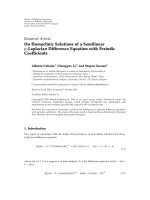
Figures 3 and 4 show the gain in step size expressed
by (21)fordifferent decimation factors (N) and different
lengths of the adaptive filter (L).
Basically, the analytical expressions and figures show that
the step size can be multiplied by N as long as certain fre-
quencies, at which a notch in the gain in step size appears,
are avoided. The location of these critical frequencies, as well
as the number and width of the notches, will be analyzed as
a function of the sampling frequency F
s
, the length of the
adaptive filter L, and the decimation factor N. According to
(19)and(21), with increasing decimation factor N, the step
size can be multiplied by N and,asaresultofthataffordable
compensation, the PU sequential algorithm convergence is as
fast as the full update FxLMS algorithm as long as the unde-
sired disturbance is free of components located at the notches
of the g ain in step size.
Figure 3 shows that the total number of equidistant
notches appearing in the gain in step size is (N
1). In fact,

the notches appear at the frequencies given by
f
k notch
= k
F
s
2N
, k
= 1, , N 1. (22)
It is important to avoid the undesired sinusoidal noise be-
ing at the mentioned notches because the gain in step size is
smaller there, with the subsequent reduction in convergence
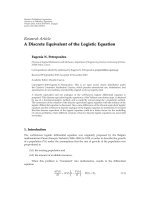
rate. As far as the width of the notches is concerned, Figure 4
(where the decimation factor N
= 2) shows that the smaller
the length of the filter, the wider the main notch of the gain
in step size. In fact, if L/N is an integer, the width between
first zeros of the main notch can be expressed as
width
=
F
s
L
. (23)
Simulations and practical experiments confirm that at these
problematic frequencies, the gain in step size cannot be ap-
plied at its maximum value N.
If it were not possible to avoid the presence of some har-
monic at a frequency where there were a notch in the gain,
the proposed strategy could be combined with the filtered-

error least mean-square (FeLMS) algorithm [13, Chapter 3].
The FeLMS algorithm is based on a shaping filter C(z) placed
in the error path and in the filtered reference path. The trans-
fer function C(z) is the inverse of the desired shape of the
residual noise. Therefore, C(z) must be designed as a comb
filter with notches at the problematic frequencies. As a re-
sult of that, the harmonics at those frequencies would not be
canceled. Nevertheless, if a noise component were to fall in a
notch, using a smaller step size could be preferable to using
the FeLMS, considering that typically it is more important to
cancel all noise disturbance frequencies rather than obtain-
ing the fastest possible convergence rate.
3. NOISE ON THE WEIGHT VECTOR SOLUTION
AND EXCESS MEAN-SQUARE ERROR
The aim of this section is to prove that the full-strength gain
in step size G
μ
= N can be applied in the context of ANC
Pedro Ramos et al. 7
0.40.30.20.10
Normalized frequency
0
0.5
1
1.5
2
Gain in step size
(a) L = 256, N = 1
0.40.30.20.10
Normalized frequency

0
0.5
1
1.5
2
2.5
3
Gain in step size
(b) L = 256, N = 2
0.40.30.20.10
Normalized frequency
0
1
2
3
4
5
Gain in step size
(c) L = 256, N = 4
0.40.30.20.10
Normalized frequency
0
2
4
6
8
Gain in step size
(d) L = 256, N = 8
Figure 3: Gain in step size for a single tone and different decimation factors N = 1, 2, 4, 8.
0.50.40.30.20.10

Normalized frequency
1
1.2
1.4
1.6
1.8
2
2.2
Gain in step size
Gain in step size for different
lengths of the adaptive filter, N
= 2
L
= 128
L
= 32
L
= 8
Figure 4: Gain in step size for a single tone and different filter
lengths L
= 8, 32, 128 with decimation factor N = 2.
systems controlled by the filtered-x sequential LMS algo-
rithm without an additional increase in mean-square error
caused by the noise on the weight vector solution. We begin
with an analysis of the trace of the autocorrelation matrix
of an N-decimated signal x
N
(n), which is included to pro-
vide mathematical support for subsequent parts. The second
part of the section revises the analysis performed by Widrow

and Stearns of the effect of the g radient noise on the LMS
algorithm [16, Chapter 6]. The section ends with the exten-
sion to the G
μ
-FxSLMS algorithm of the previously outlined
analysis.
3.1. Properties of the trace of an N-decimated
autocorrelation matrix
Let the L
1vectorx(n) represent the elements of a signal.
To show the composition of the vector x(n), we write
x(n)
=

x( n), x(n 1), , x(n L +1)

T
. (24)
The expectation of the outer product of the vector x(n)with
itself determines the L
L autocorrelation matrix R of the
8 EURASIP Journal on Audio, Speech, and Music Processing
signal
R
= E

x(n)x
T
(n)


=
⎡
⎢
⎢
⎢
⎢
⎢
⎢
⎢
⎢
⎢
⎣
r
xx
(0) r
xx
(1) r
xx
(2) r
xx
(L 1)
r
xx
(1) r
xx
(0) r
xx
(1) r
xx
(L 2)

r
xx
(2) r
xx
(1) r
xx
(0) r
xx
(L 3)
.
.
.
.
.
.
.
.
.
.
.
.
.
.
.
r
xx
(L 1) r
xx
(L 2) r
xx

(L 3) r
xx
(0)
⎤
⎥
⎥
⎥
⎥
⎥
⎥
⎥
⎥
⎥
⎦
.
(25)
The N-decimated signal x
N
(n) is obtained from vector
x(n) by multiplying x(n) by the auxiliary matrix I
(N)
k
,
x
N
(n) = I
(N)
k
x(n), k = 1+n mod N, (26)
where I

(N)
k
is obtained from the identity matrix I of dimen-
sion L
L by zeroing out some elements in I. The first nonnull
element on its main diagonal appears at the kth position and
the superscr ipt (N) is intended to denote the fact that two
consecutive nonzero elements on the main diagonal are sep-
arated by N positions. The auxiliary matrix I
(N)
k
is explicitly
expressed as
I
(N)
k
=
⎛
⎜
⎜
⎜
⎜
⎜
⎜
⎜
⎜
⎜
⎜
⎜
⎜

⎜
⎜
⎜
⎜
⎜
⎜
⎜
⎜
⎜
⎜
⎜
⎜
⎜
⎜
⎜
⎝
0
.
.
.
k
1
0
10
0
N
.
.
.
0

- 1
00
.
.
.
0
⎞
⎟
⎟
⎟
⎟
⎟
⎟
⎟
⎟
⎟
⎟
⎟
⎟
⎟
⎟
⎟
⎟
⎟
⎟
⎟
⎟
⎟
⎟
⎟

⎟
⎟
⎟
⎟
⎠
. (27)
As a result of (26), the autocorrelation matrix R
N
of the
new signal x
N
(n) only presents nonnull elements on its main
diagonal and on any other diagonal parallel to the main di-
agonal that is separated from it by kN positions, k being any
integer. Thus,
R
N
= E

x
N
(n)x
T
N
(n)

=
1
N
⎡

⎢
⎢
⎢
⎢
⎢
⎢
⎢
⎢
⎢
⎢
⎢
⎢
⎢
⎢
⎢
⎢
⎢
⎢
⎢
⎢
⎢
⎣
r
xx
(0) 0 0 r
xx
(N) r
xx
(2N)
.

.
.
0 r
xx
(0) 0
.
.
.
0 r
xx
(N)
.
.
.
.
.
.
.
.
.0r
xx
(0) 0
.
.
.
0
.
.
.
0

.
.
.
0 r
xx
(0) 0
.
.
.
r
xx
(N)
r
xx
(N)0
.
.
.
0 r
xx
(0) 0
.
.
.
0
.
.
. r
xx
(N)0

.
.
.
0 r
xx
(0)
.
.
.
r
xx
(2N)
.
.
.
.
.
.
0
.
.
.
00
.
.
.
r
xx
(N)0 r
xx

(0)
⎤
⎥
⎥
⎥
⎥
⎥
⎥
⎥
⎥
⎥
⎥
⎥
⎥
⎥
⎥
⎥
⎥
⎥
⎥
⎥
⎥
⎥
⎦
.
(28)
The matrix R
N
can be expressed in terms of R as
R

N
=
1
N
N

i=1
I
(N)
i
RI
(N)
i
. (29)
We define the diagonal matrix Λ with main diagonal
comprised of the L eigenvalues of R.IfQ is a matrix whose
columns are the eigenvectors of R,wehave
Λ
= Q
1
RQ =
⎛
⎜
⎜
⎜
⎜
⎜
⎜
⎜
⎜

⎜
⎜
⎝
λ
1
0 0
0
.
.
.
.
.
.
0
.
.
.
.
.
.
.
.
.
λ
i
.
.
.
.
.

.
.
.
.0
.
.
.
.
.
.
0
0
0 λ
L
⎞
⎟
⎟
⎟
⎟
⎟
⎟
⎟
⎟
⎟
⎟
⎠
. (30)
The trace of R is defined as the sum of its diagonal elements.
The trace can also be obtained from the sum of its eigenval-
ues, that is,

trace(R)
=
L

i=1
r
xx
(0) = trace(Λ) =
L

i=1
λ
i
. (31)
The relation between the traces of R and R
N
is given by
trace

R
N

=
L

i=1
r
xx
(0)
N

=
trace(R)
N
. (32)
3.2. Effects of the gradient noise on the LMS algorithm
Let the vector w(n) represent the weights of the adaptive fil-
ter, which are updated according to the LMS algorithm as
follows:
w(n +1)
= w ( n)
μ
2

(n) = w(n)+μe(n)x(n), (33)
where μ is the step size,

(n) is the gradient estimate at the
nth iteration, e(n) is the error at the previous iteration, and
x(n) is the vector of input samples, also called the regressor
signal.
We define v(n) as the deviation of the weight vector from
its optimum value
v(n)
= w ( n) w
opt
(34)
and v
(n) as the rotation of v(n) by means of the eigenvector
matrix Q,
v

(n) = Q
1
v(n) = Q
1

w(n) w
opt

. (35)
In order to give a measure of the difference between
actual and optimal performance of an adaptive algorithm,
two parameters can be taken into account: excess mean-
square error and misadjustment. The excess mean-square er-
ror ξ
excess
is the average mean-square error l ess the minimum
mean-square error, that is,
ξ
excess
= E

ξ(n)

ξ
min
. (36)
Pedro Ramos et al. 9
The misadjustment M is defined as the excess mean-square
error divided by the minimum mean-square error
M

=
ξ
excess
ξ
min
=
E

ξ(n)

ξ
min
ξ
min
. (37)
Random weight variations around the optimum v alue of
the filter cause an increase in mean-square error. The average
of these increases is the excess mean-square error. Widrow
and Stearns [16, Chapters 5 and 6] analyzed the steady-state
effects of gradient noise on the weight vector solution of the
LMS algorithm by means of the definition of a vector of noise
n(n) in the gradient estimate at the nth iteration. It is as-
sumed that the LMS process has converged to a steady-state
weight vector solution near its optimum and that the true
gradient
(n) is close to zero. Thus, we write
n(n)
=

(n) (n) =


(n) = 2e(n)x ( n). (38)
The weight vector covariance in the principal axis coordinate
system, that is, in primed coordinates, is related to the co-
variance of the noise as follows [16, Chapter 6]:
cov

v (n)

=
μ
8

Λ
μ
2
Λ
2

1
cov

n (n)

=
μ
8

Λ
μ

2
Λ
2

1
cov

Q
1
n(n)

=
μ
8

Λ
μ
2
Λ
2

1
Q
1
E

n(n)n
T
(n)


Q.
(39)
In practical situations, (μ/2)Λ tends to be negligible with re-
spect to I, so that (39) simplifies to
cov

v (n)

≈
μ
8
Λ
1
Q
1
E

n(n)n
T
(n)

Q. (40)
From (38), it can be shown that the covariance of the gra-
dient estimation noise of the LMS algorithm at the minimum
point is related to the autocorrelation input matrix according
to (41)
cov

n(n)


=
E

n(n)n
T
(n)

=
4E

e
2
(n)

R. (41)
In (41), the error and the input vector are considered statisti-
cally independent because at the minimum point of the error
surface both signals are orthogonal.
To s um up, ( 40)and(41) indicate that the measurement
of how close the LMS algorithm is to optimality in the mean-
square error sense depends on the product of the step size
and the autocorrelation matrix of the regressor signal x(n).
3.3. Effects of gradient noise on the filtered-x
sequential LMS algorithm
At this point, the goal is to carry out an analysis of the effect
of gradient noise on the weight vector solution for the case
of the G
μ
-FxSLMS algorithm in a similar manner as in the
previous section.

The weights of the adaptive filter when the G
μ
-FxSLMS
algorithm is used are updated according to the recursion
w(n +1)
= w ( n)+G
μ
μe(n)I
(N)
1+n modN
x (n), (42)
where I
(N)
1+n modN
is obtained from the identity matrix as ex-
pressedin(27). The gradient estimation noise of the filtered-
x sequential LMS algorithm at the minimum point, where
the true gradient is zero, is given by
n(n)
=

(n) = 2e(n)I
(N)
1+n modN
x (n). (43)
Considering PU, only L/N terms out of the L-length noise
vector are nonzero at each iteration, giving a smaller noise
contribution in comparison with the LMS algorithm, which
updates the whole filter.
The weight vector covariance in the principal axis coor-

dinate system, that is, in primed coordinates, is related to the
covariance of the noise as follows:
cov

v (n)

=
G
μ
μ
8

Λ
G
μ
μ
2
Λ
2

1
cov

n (n)

=
G
μ
μ
8


Λ
G
μ
μ
2
Λ
2

1
cov

Q
1
n(n)

=
G
μ
μ
8

Λ
G
μ
μ
2
Λ
2


1
Q
1
E

n(n)n
T
(n)

Q.
(44)
Assuming that (G
μ
μ/2)Λ is considerably less than I, then (44)
simplifies to
cov

v (n)

≈
G
μ
μ
8
Λ
1
Q
1
E


n(n)n
T
(n)

Q. (45)
The covariance of the gradient estimation error noise
when the sequential PU is used can be expressed a s
cov

n(n)

=
E

n(n)n
T
(n)

=
4E

e
2
(n)I
(N)
1+n modN
x (n)x
T
(n)I
(N)

1+n modN

=
4E

e
2
(n)

E

I
(N)
1+n modN
x (n)x
T
(n)I
(N)
1+n modN

=
4E

e
2
(n)

1
N
N


i=1
I
(N)
i
RI
(N)
i
= 4E

e
2
(n)

R
N
.
(46)
In (46), statistical independence of the error and the input
vector has been assumed at the minimum point of the error
surface, where both signals are orthogonal.
According to (32), the comparison of (40)and(45)—
carried out in terms of the trace of the autocorrelation
matrices—confirms that the contribution of the gradient es-
timation noise is N times weaker for the sequential LMS al-
gorithm than for the LMS. This reduction compensates the
eventual increase in the covariance of the weight vector in the
principal axis coordinate system expressed in (45) when the
maximum gain in step size G
μ

= N is applied in the context
of the G
μ
-FxSLMS algorithm.
10 EURASIP Journal on Audio, Speech, and Music Processing
40003000200010000
Frequency (Hz)
4
3
2
1
0
1
P( f )
(a)
40003000200010000
Frequency (Hz)
50
40
30
20
10
0
10
S( f )
(b)
40003000200010000
Frequency (Hz)
50
40

30
20
10
0
10
S
e
( f )
(c)
4003002001000
Frequency (Hz)
40
20
0
20
Power spectral density (dB)
(d)
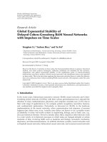
Figure 5: Transfer function magnitude of (a) primary path P(z), (b) secondary path S(z), and (c) offline estimate of the secondary path
used in the simulated model, (d) power spectr al density of periodic disturbance consisting of two tones of 62.5 Hz and 187.5 Hz in additive
white Gaussian noise.
4. EXPERIMENTAL RESULTS
In order to assess the effectiveness of the G
μ
-FxSLMS algo-
rithm, the proposed strategy was not only tested by simula-
tion but was also evaluated in a practical DSP-based imple-
mentation. In both cases, the results confirmed the expected
behavior: the performance of the system in terms of conver-
gence rate and residual error is as good as the performance
achieved by the FxLMS algorithm, even while the number of

operations per iteration is significantly reduced due to PU.
4.1. Computer simulations
This section describes the results achieved by the G
μ
-FxSLMS
algorithm by means of a computer model developed in MAT-
LAB on the theoretical basis of the previous sections. The
model chosen for the computer simulation of the first ex-
ample corresponds to the 1
1 1 (1 reference microphone,
1 secondary source, and 1 error microphone) arrangement
described in Figure 1(a). Transfer functions of the primary
path P(z) and secondary path S(z) are shown in Figures 5(a)
and 5(b), respectively. The filter modeling the primary path
is a 64th-order FIR filter. The secondary path is modeled—
by a 4th-order elliptic IIR filter—as a high pass filter whose
cut-off frequency is imposed by the poor response of the
loudspeakers at low frequencies. The offline estimate of the
secondary path was carried out by an adaptive FIR filter of
200 coefficients updated by the LMS algorithm, as a classi-
cal problem of system identification. Figure 5(c) shows the
transfer function of the estimated secondary path. The sam-
pling frequency (8000 samples/s) as well as other parameters
were chosen in order to obtain an approximate model of the
real implementation. Finally, Figure 5(d) shows the power
spectr al density of x(n), the reference signal for the undesired
disturbance which has to be canceled
x( n)
= cos(2π62.5n) + cos(2π187.5n)+η(n), (47)
where η(n) is an additive white Gaussian noise of zero mean

whose power is
E

η
2
(n)

= σ
2
η
= 0.0001 ( 40 dB). (48)
After convergence has been achieved, the power of the resid-
ual error corresponds to the power of the random compo-
nent of the undesired disturbance.
Thelengthoftheadaptivefilterisof256coefficients. The
simulation was carried out as follows: the step size was set to
zero during the first 0.25 seconds; after that, it is set to 0.0001
Pedro Ramos et al. 11
4002000
Frequency (Hz)
0
0.5
1
1.5
2
Gain in step size
(a) N = 1
4002000
Frequency (Hz)
0

0.5
1
1.5
2
2.5
3
Gain in step size
(b) N = 2
4002000
Frequency (Hz)
0
2
4
6
8
Gain in step size
(c) N = 8
4002000
Frequency (Hz)
0
5
10
15
20
25
30
Gain in step size
(d) N = 32
4002000
Frequency (Hz)

0
10
20
30
40
50
60
Gain in step size
(e) N = 64
4002000
Frequency (Hz)
0
20
40
60
80
Gain in step size
(f) N = 80
Figure 6: Gain in step size over the frequency band of interest—from 0 to 400 Hz—for differentvaluesofthedecimationfactorN (N =
1, 2, 8, 32, 64, 80).
and the adaptive process starts. The value μ = 0.0001 is near
the maximum stable step size when a decimation factor N
=
1 is chosen.
The performance of the G
μ
-FxSLMS algorithm was tested
for different values of the decimation factor N. Figure 6
shows the gain in step size over the frequency band of in-
terest for different values of the parameter N. The gain in

step size at the frequencies 62.5 Hz and 187.5Hzaremarked
with two circles over the curves. The exact location of the
notchesisgivenby(22). On the basis of the position of the
notches in the gain in step size and the spectral distribution
of the undesired noise, the decimation factor N
= 64 is ex-
pected to be critical because, according to Figure 6, the full-
strength gain G
μ
= N = 64 cannot be applied at the fre-
quencies 62.5 Hz and 187.5 Hz; both frequencies correspond
exactly to the sinusoidal components of the periodic distur-
bance. Apart from the case N
= 64 the gain in step size is free
of notches at both of these frequencies.
Convergence curves for different values of the decima-
tion factor N are shown in Figure 7. The numbers that ap-
pear over the figures correspond to the mean-square error
computed over the last 5000 iterations. The residual error is
expressed in logarithmic scale as the r a tio of the mean-square
error and a signal of unitary power. As expected, the conver-
gence rate and residual error are the same in all cases except
when N
= 64. For this value, the active noise control system
diverges. In order to make the system converge when N
= 64,
it is necessar y to decrease the gain in step size to a maximum
value of 32 with a subsequent reduction in convergence rate.
The second example compares the theoretical gain in step
size with the increase obtained by MATLAB simulation. The

model of this example corresponds, as in the previous exam-
ple, to the 1
1 1 arrangement described in Figure 1.In
this example, the reference is a single sinusoidal signal whose
frequency varied in 20 Hz steps from 40 to 1560 Hz. The sam-
pling frequency of the model is 3200 samples/s. Primary and
secondary paths—P(z)andS(z)—are pure delays of 300 and
40 samples, respectively. The output of the primary path is
mixed with additive white Gaussian noise providing a sig nal-
to-noise ratio of 27 dB. It is assumed that the secondary path
has been exactly estimated. In order to provide very accurate
results, the increase in step size between every two consec-
utive simulations looking for the bound is less than 1/5000
the final value of the step size that ensures convergence. The
12 EURASIP Journal on Audio, Speech, and Music Processing
0.350.30.250.2
Time (s)
0
0.5
1
1.5
2
2.5
Instantaneous error power
40.8dB
(a) N = 1
0.350.30.250.2
Time (s)
0
0.5

1
1.5
2
2.5
Instantaneous error power
40.8dB
(b) N = 2
0.350.30.250.2
Time (s)
0
0.5
1
1.5
2
2.5
Instantaneous error power
40.7dB
(c) N = 8
0.350.30.250.2
Time (s)
0
0.5
1
1.5
2
2.5
Instantaneous error power
40.6dB
(d) N = 32
0.350.30.250.2

Time (s)
0
0.5
1
1.5
2
2.5
Instantaneous error power
112 dB
(e) N = 64
0.350.30.250.2
Time (s)
0
0.5
1
1.5
2
2.5
Instantaneous error power
40.6dB
(f) N = 80
Figure 7: Evolution of the instantaneous error power in an ANC system using the G
μ
-FxSLMS algorithm for different values of the decima-
tion factor N (N
= 1, 2, 8, 32, 64, 80). In all cases, the gain in step size was set to the maximum value G
μ
= N.
decimation factor N of this example was set to 4. Figure 8
compares the predicted gain in step size with the achieved

results. As expected, the experimental gain in step size is 4,
apart from the notches that appear at 400, 800, and 1200 Hz.
4.2. Practical implementation
The G
μ
-FxSLMS algorithm was implemented in a 1 2 2ac-
tive noise control system aimed at attenuating engine noise at
the front seats of a Nissan Vanette. Figure 9 shows the phys-
ical arrangement of elec troacoustic elements. The adaptive
algorithm was developed on a hardware platform based on
the DSP TMS320C6701 from Texas Instruments [18].
The length of the adaptive filter (L) for the G
μ
-FxSLMS
algorithm was set to 256 or 512 coefficients (depending on
the spectr al characteristics of the undesired noise and the de-
gree of attenuation desired), the length of the estimate of the
secondary path (L
s
) was set to 200 coefficients, and the dec-
imation factor and the gain in step size were N
= G
μ
= 8.
The sampling frequency was F
s
= 8000 samples/s. From the
parameters selected, one can derive, according to (22), that
the first notch in the gain in step size is located at 500 Hz.
The system effectively cancels the main harmonics of the en-

gine noise. Considering that the loudspeakers have a low cut-
off frequency of 60 Hz, the controller cannot attenuate the
components below this frequency. Besides, the ANC system
finds more difficulty in the attenuation of closely spaced fre-
quency harmonics (see Figure 10(a)). This problem can be
avoided by increasing the number of coefficients of the adap-
tive filter; for instance, from L
= 256 to 512 coefficients (see
Figure 10(b)).
In order to carry out a performance comparison of the
G
μ
-FxSLMS algorithm with increasing value in the decima-
tion term N—and subsequently in gain in step size G
μ
—
it is essential to repeat the experiment with the same un-
desired disturbance. So to avoid inconsistencies in level
and frequency, instead of starting the engine, we have pre-
viously recorded a signal consisting of several harmon-
ics (100, 150, 200, and 250 Hz). An omnidirectional source
(Br
¨
uel & Kjaer Omnipower 4296) placed inside the van is fed
with this signal. Therefore, a comparison could be made un-
der the same conditions. The ratio—in logarithmic scale—
of the mean-square error and a signal of unitary power that
appears over the graphics was calculated averaging the last
Pedro Ramos et al. 13
16001400120010008006004002000

Frequency (Hz)
0
0.5
1
1.5
2
2.5
3
3.5
4
4.5
5
Gain in step size
Simulated versus theoretical gain
in step size, N
= 4, L = 32
Simulation
Theoretical
Figure 8: Theoretically predicted gain in step size versus simulated
results achieved in a modeled ANC system using the G
μ
-FxSLMS
algorithm.
Secondary
source
Error
microphone
Engine
noise
Reference

microphone
Error
microphone
Secondary
source
Figure 9: Arrangement of the electroacoustic elements inside the
van.
iterations shown. In this case, the length of the adaptive filter
was set to 256 coefficients, the length of the estimate of the
secondary path (L
s
) was set to 200 coefficients, and the deci-
mation factor and the gain in step size were set to N
= G
μ
=
1, 2, 4, and 8. The sampling frequency was F
s
= 8000 sam-
ples/s and the first notch in the gain in step size appeared at
500 Hz, well above the spectral location of the undesired dis-
turbance. From the experimental results shown in Figure 11,
the application of the full-st rength gain in step size when
the decimation factor is 2, 4, or 8 reduces the computational
costs without degrading in any sense the performance of the
system with respect to the full update algorithm.
Taking into account that the 2-channel ANC system im-
plementing the G
μ
-FxSLMS algorithm inside the van ignored

400350300250200150100500
Frequency (Hz)
50
40
30
20
10
0
10
Power spectrum magnitude (dB)
ANC off
ANC on
(a) L = 256, N = 8
400350300250200150100500
Frequency (Hz)
50
40
30
20
10
0
10
Power spectrum magnitude (dB)
ANC off
ANC on
(b) L = 512, N = 8
Figure 10: Power spectral density of the undesired noise (dotted)
and of the residual error (solid) for the real cancelation of engine
noise at the driver location. The decimation factor is N
= 8 and the

length of the adaptive filter is (a) L
= 256 and (b) L = 512.
cross terms, the expressions given by Tables 1 and 2 show that
approximately 32%, 48%, and 56% of the high-level multi-
plications can be saved when the decimation factor N is set
to 2, 4, and 8, respectively.
Although reductions in the number of operations are an
indication of the computational efficiency of an algorithm,
such reductions may not directly tr anslate to a more effi-
cient real-time DSP-based implementation on a hardware
platform. To accurately gauge such issues, one must consider
the freedoms and constraints that a platform imposes in the
14 EURASIP Journal on Audio, Speech, and Music Processing
2.521.510.50
Time (s)
0
0.04
Error power
40.16 dB
(a) N = 1
2.521.510.50
Time (s)
0
0.04
Error power
40.18 dB
(b) N = 2
2.521.510.50
Time (s)
0

0.04
Error power
41.7dB
(c) N = 4
2.521.510.50
Time (s)
0
0.04
Error power
40.27 dB
(d) N = 8
Figure 11: Error convergence of the real implementation of the G
μ
-
FxSLMS algorithm with increasing value of the decimation factor
N. The system deals with a previously recorded signal consisting of
harmonics at 100, 150, 200, and 250 Hz.
real implementation, such as parallel operations, addressing
modes, registers available, or number of arithmetic units. In
our case, the control strategy and the assembler code was de-
veloped trying to take full advantage of these aspects [5].
5. CONCLUSIONS
This work presents a contribution to the selection of the step
size used in the sequential partial update LMS and FxLMS
adaptive algorithms. The deterministic periodic input signal
case is studied and it is verified that under certain conditions
the stability range of the step size is increased compared to
the full update LMS and FxLMS.
The algorithm proposed here—filtered-x sequential LMS
with gain in step size (G

μ
-FxSLMS)—is based on sequential
PU of the coefficients of a filter and on a controlled increase
in the step size of the adaptive algorithm. It can be used in ac-
tive noise control systems focused on the attenuation of pe-
riodic disturbances to reduce the computational costs of the
control system. It is theoretically and experimentally proved
that the reduction of the computational complexity is not
achieved at the expense of slowing down the convergence rate
or of increasing the residual error.
The only condition that must be accomplished to take
full advantage of the algorithm is that some frequencies
should be avoided. These problematic frequencies corre-
spond to notches that appear at the gain in step size. Their
width and exact location depend on the system parameters.
Simulations and experimental results confirm the bene-
fits of this strategy when it is applied in an active noise con-
trol system to attenuate periodic noise.
ACKNOWLEDGMENT
This work was partially supported by CICYT of Spanish Gov-
ernment under Grant TIN2005-08660-C04-01.
REFERENCES
[1] P. Lueg, “Process of silencing sound oscillations,” U.S. Patent
no. 2.043.416, 1936.
[2] D. R. Morgan, “Analysis of multiple correlation cancellation
loops with a filter in the auxiliary path,” IEEE Transactions on
Acoustics, Speech, and Signal Processing, vol. 28, no. 4, pp. 454–
467, 1980.
[3] B. Widrow, D. Shur, and S. Shaffer, “On adaptive inverse con-
trol,” in Proceedings of the15th Asilomar Conference on Circuits,

Systems, and Computers, pp. 185–195, Pacific Grove, Calif,
USA, November 1981.
[4] J. C. Burgess, “Active adaptive sound control in a duct: a com-
puter simulation,” JournaloftheAcousticalSocietyofAmerica,
vol. 70, no. 3, pp. 715–726, 1981.
[5] P.Ramos,R.Torrubia,A.L
´
opez, A. Salinas, and E. Masgrau,
“Computationally efficient implementation of an active noise
control system based on partial updates,” in Proceedings of the
International Symposium on Active Control of Sound and Vibra-
tion (ACTIVE ’04), Williamsburg, Va, USA, September 2004,
paper 003.
[6] S. C. Douglas, “Adaptive filters employing par tial updates,”
IEEE Transactions on Circuits and Systems II: Analog and Digi-
tal Signal Processing, vol. 44, no. 3, pp. 209–216, 1997.
[7] T. Aboulnasr and K. Mayyas, “Selective coefficient update of
gradient-based adaptive algorithms,” in Proceedings of IEEE In-
ternational Conference on Acoustics, Speech and Signal Process-
ing (ICASSP ’97), vol. 3, pp. 1929–1932, Munich, Germany,
April 1997.
[8] K. Do
ˇ
ganc¸ay and O. Tanrikulu, “Adaptive filtering algorithms
with selective partial updates,” IEEE Transactions on Circuits
and Systems II: Analog and Digital Signal Processing, vol. 48,
no. 8, pp. 762–769, 2001.
[9] J. Sanubari, “Fast convergence LMS adaptive filters employ-
ing fuzzy partial updates,” in Proceedings of IEEE Conference
on Convergent Technologies for Asia-Pacific Region (TENCON

’03), vol. 4, pp. 1334–1337, Bangalore, India, October 2003.
[10] P. A. Naylor, J. Cui, and M. Brookes, “Adaptive algorithms for
sparse echo cancellation,” Signal Processing,vol.86,no.6,pp.
1182–1192, 2006.
[11] S. M. Kuo, M. Tahernezhadi, and W. Hao, “Convergence anal-
ysis of narrow-band active noise control system,” IEEE Trans-
actions on Circuits and Systems II: Analog and Digital Signal
Processing, vol. 46, no. 2, pp. 220–223, 1999.
Pedro Ramos et al. 15
[12] E. Bjarnason, “Analysis of the filtered-X LMS algorithm,” IEEE
Transactions on Speech and Audio Processing, vol. 3, no. 6, pp.
504–514, 1995.
[13] S. M. Kuo and D. R. Morgan, Active Noise Control Systems: Al-
gorithms and DSP Implementations, John Wiley & Sons, New
York, NY, USA, 1996.
[14] L. Vicente and E. Masgrau, “Novel FxLMS convergence condi-
tion with deterministic reference,” IEEE Transactions on Signal
Processing, vol. 54, no. 10, pp. 3768–3774, 2006.
[15] S. J. Elliott, Sign al Processing for Active Control,Academic
Press, London, UK, 2001.
[16] B. Widrow and S. D. Stearns, Adaptive Signal Processing,Pren-
tice Hall, Englewood Cliffs, NJ, USA, 1985.
[17] S. Haykin, Adaptive Filter Theory, Prentice Hall, Upper Saddle
River, NJ, USA, 2002.
[18] Texas Instruments Digital Signal Processing Products, “TMS-
320C6000 CPU and Instruction Set Reference Guide,” 1999.