Báo cáo hóa học: " Perfect Reconstruction Conditions and Design of Oversampled DFT-Modulated Transmultiplexers" ppt
Bạn đang xem bản rút gọn của tài liệu. Xem và tải ngay bản đầy đủ của tài liệu tại đây (906.07 KB, 14 trang )
Hindawi Publishing Corporation
EURASIP Journal on Applied Signal Processing
Volume 2006, Article ID 15756, Pages 1–14
DOI 10.1155/ASP/2006/15756
Perfect Reconstruction Conditions and Design of Oversampled
DFT-Modulated Transmultiplexers
Cyrille Siclet,
1
Pierre Siohan,
2
and Didier Pinchon
3
1
Laboratoire des Images et des Signaux (LIS), Universit
´
e Joseph Fourier, 38402 Saint Martin d’H
`
eres Cedex, France
2
Laboratoire RESA/BWA, Division Recherche et D
´
eveloppement, France T
´
el
´
ecom, 4 r ue du Clos Courtel,
35512 Cesson S
´
evign
´
eCedex,France
3
Laboratoire Math
´
ematiques pour l’Industrie et la Physique (MIP), Universit
´
e Paul Sabatier, Toulouse 3,
31062 Toulouse Cedex 9, France
Received 1 September 2004; Revised 12 July 2005; Accepted 19 July 2005
This paper presents a theoretical analysis of oversampled complex modulated transmultiplexers. The perfect reconstruction (PR)
conditions are established in the polyphase domain for a pair of biorthogonal prototype filters. A decomposition theorem is pro-
posed that allows it to split the initial system of PR e quations, t hat can be huge, into small independent subsystems of equations.
In the orthogonal case, it is shown that these subsystems can be solved thanks to an appropriate angular parametrization. This
parametrization is efficiently exploited afterwards, using the compact representation we recently introduced for critically dec-
imated modulated filter banks. Two design criteria, the out-of-band energy minimization and the time-frequency localization
maximization, are examined. It is shown, with various design examples, that this approach allows the design of oversampled mod-
ulated transmultiplexers, or filter banks with a thousand carriers, or subbands, for rational oversampling ratios corresponding to
low redundancies. Some simulation results, obtained for a transmission over a flat fading channel, also show that, compared to the
conventional OFDM, these designs may reduce the mean square error.
Copyright © 2006 Cyrille Siclet et al. This is an open access article distributed under the Creative Commons Attribution License,
which permits unrestricted use, distribution, and reproduction in any medium, provided the original work is properly cited.
1. INTRODUCTION
Since the mid-nineties, oversampled filter banks have re-
ceived a considerable amount of attention. Original ly, most
of the studies were devoted to subband encoder structures
corresponding to a serial concatenation of an analysis and
synthesis filter bank having a decimation and expansion fac-
tor inferior to the number of filters [1]. In this paper, as
in [2–6], we are mainly interested in the converse situation,
which corresponds to a transmultiplexer where the transmit-
ter is composed of a synthesis filter bank (SFB) generating
the t ransmitted signal that is afterwards estimated by a re-
ceiver composed of an analysis filter bank (AFB). Oversam-
pling then means that the expansion and decimation r a tios
have to be higher than the number of subbands in order to
get a perfect estimation of the tr ansmitted symbols, that is,
the equivalent of the perfect reconstruction (PR) conditions
used in the filter bank context.
In general, in the oversampled case, a duality relationship
between filter banks and t ransmultiplexers, such as the one
proved in [7] for critically decimated systems, does not exist.
However , if we restrict ourselves to the class of oversampled
filter banks using an exponential modulation based on the
discrete Fourier transform (DFT), under certain conditions,
duality relations can still be established. As in [2, 3], in the or-
thogonal case, they may be proved showing the equivalence
of the PR conditions. They can also appear in a more gen-
eral setting as a consequence of the duality between frames
and biorthogonal families in the Weyl-Heisenberg (Gabor)
systems theory, see [8] and references therein. This duality
naturally gives a more general impact to the family of over-
sampled DFT-modulated filter banks.
In a transmission context, oversampled DFT-modulated
filter banks can be seen as a discrete-time approach to get
efficient multicarri er transmission systems. In this field, for
the time being, the reference is still the orthogonal frequency
division multiplex (OFDM), also known as the discrete mul-
titone (DMT) for wired transmission. Indeed, OFDM/DMT
is now part of various transmission standards related to wire-
less and wired links. Nevertheless, OFDM presents some
weaknesses which explain why several studies are still under-
taken to propose efficient alternatives. OFDM corresponds
to a critically decimated DFT-modulated filter bank, there-
fore it cannot have a good frequency localization [9]. This
2 EURASIP Journal on Applied Signal Processing
directly leads to one of the main drawbacks of the conven-
tional OFDM with DFT filters whose attenuation is approx-
imately limited to the 13 dB provided by a rectangular win-
dow shaping. Higher attenuation levels are desirable as illus-
trated, for example, in [10] in the case of transmission over
very high-bit-rate digital subscriber lines (VDSL). Depend-
ing on the application at hand, they may be required at the
transmitter, to limit the out-of-band energy, and/or at the re-
ceiver for combatting narrowband interference or frequency
shifts between the transmitter and the receiver. On the other
hand, it is now widely recognized that time-frequency lo-
calization is an essential feature for transmission over time-
frequency dispersive channels.
A first alternative to introduce an efficient pulse shap-
ing is based on a variant of OFDM where the modulation
of each carrier is properly modified. Instead of using a clas-
sical quadrature amplitude modulation (QAM), each car-
rier is modulated using a staggered offset QAM (OQAM),
leading to a modulation now known as OFDM/OQAM. In
theory, OFDM/OQAM allows it to get a maximum spec-
tral efficiency. Recently, there were several proposals elabo-
rated either using continuous-time [11–13] or discrete-time
[14, 15] formalisms, some of these orthogonal schemes are
generalized afterwards to get biorthogonal modulation, that
is, BFDM/OQAM [8, 16]. But then, the introduction of an
offset complicates the channel estimation task.
Another alternative in order to introduce pulse shap-
ing, the one developed in the present paper, is to build
oversampled multicarrier systems. Then, channel estimation
becomes easier, but on the other hand, oversampling also
means added redundancy, and consequently loss of spectral
efficiency. For instance, to be competitive with existing sys-
tems, oversampled transmultiplexers must not add more re-
dundancy than that introduced in a conventional OFDM sys-
tem with the cyclic prefix, that is, an extension of the symbol
duration that generally only corresponds to a small fraction
of the overall useful symbol time duration. Furthermore, as
multicarrier systems often require a high (hundreds) or a
very high (thousands) number of carriers, we need a de-
sign method that satisfies both requirements. Several ap-
proaches have been proposed to provide appropriate answers
to these problems. They can again be classified according
to the type of formalism, continuous-time or discrete-time,
which is used to get the desired pulse shapes. References
[8, 17–19] share a common feature that is to propose proto-
type functions for Weyl-Heisenberg (or Gabor) systems with
good time-frequency localization. Furthermore in [18, 19],
optimization of the pulse shapes is carried out with respect
to characteristic parameters of the time-frequency dispersive
channels. However, even if in [18] the authors reach a high
spectral efficiency, with an oversampling ratio (or a redun-
dancy) of 5/4, it is for a system with only 64 carriers. As in
[2, 3], and more recently in [6], our own approach, contrary
to [17–19], is to use a discrete-time formalism with finite im-
pulse response (FIR) causal filters, and we take the recon-
struction delay into account. We then get oversampled filter
banks that can be directly implemented without a loss of the
desired properties: frequency selectivity or time-frequency
localization. Thus, in this paper, we focus on the case of over-
sampled modulated transmultiplexers. Similarly with [2, 3],
for transmultiplexers, or [1, 20] for filter banks, we use a DFT
modulation. This means that in the SFB and AFB, all filters
can be obtained by means of a multiplication of a prototype
filter by a complex exponential, thus allowing efficient fast
implementations afterwards. With this approach, the design
of spectral ly efficient multicarrier systems with a high num-
ber of carriers becomes possible, which can be seen in [3],
but more particularly in [5, 21]. This is not the case when
considering a more general filter bank structure [4]. How-
ever, even if for the DFT-modulated filter banks, the design
is reduced to one, as in [2, 3], or two [6
]prototypefilters,
it remains difficult to get systems with high number of car-
riers and low oversampling ratios. In [2, 3], the results pre-
sented for orthogonal systems are limited to 32 carriers and
an oversampling ra tio equal to 3/2. In [6], the authors op-
timize a biorthogonal transmultiplexer with 80 subcarriers
and a higher spectral efficiency, with an oversampling ratio
equal to 5/4. In this paper, we describe the different steps of
an approach that recently allowed us to obtain design results
for a similar sampling ratio but a far larger number of carri-
ers.
In particular, we investigate
(i) the necessary and sufficient PR conditions, expressed
with respect to the polyphase components of the pro-
totype filters related to oversampled BFDM/QAM sys-
tems or, equivalently, to oversampled DFT filter banks;
(ii) a simplification of the above result, w ith a splitting of
the large initial set of PR equations into a less large set
of small independent subsystems and the proof that in
a first step, only small subsystems have to be solved;
(iii) an approach which allows orthogonal systems using
FIR filters to represent the solutions of each subsystem
thanks to angular parameters;
(iv) the application to oversampled DFT transmultiplexers
of the compact representation approach, proposed in
[22], for critically decimated filter banks;
(v) a comparison between conventional and oversampled
OFDM in the case of a tra nsmission over a frequency
dispersive channel.
Our paper is organized as follows. In Section 2,we
present the general features concerning the oversampled
DFT-modulated transmultiplexer, its polyphase decompo-
sition, and its input-output relation. In Section 3,wepro-
vide the PR conditions for the biorthogonal systems and a
decomposition technique to get independent subsets of the
PR conditions. The parametrization, initially presented in
[21], is summarized in Section 4.InSection 5 ,werecallthe
basic principle of the compact representation method and
present design results, using two different optimization crite-
ria: out-of-band energy and time-frequency localization. Fi-
nally, Section 6 is devoted to the presentation of our com-
parison between conventional and oversampled OFDM in a
transmission context.
Cyr ille Siclet et al. 3
c
0,n
NF
0
(z) H
0
(z) N
c
0,n –α
c
1,n
.
.
.
NF
1
(z)
+
s[k]
z
– β
H
1
(z) N
c
1,n –α
.
.
.
c
M –1,n
NF
M –1
(z) H
M –1
(z) N
c
M –1,n– α
Figure 1: Oversampled BFDM/QAM transmultiplexer.
Notations
Z, C denote the set of integers and complex numbers, respec-
tively. l
2
(Z) corresponds to the space of square-summable
discrete-time sequences. Vec tors and matrices are denoted
with bold italic letters, for instance E. We denote discrete
filters of l
2
(Z) with lowercase letters, for instance h[n], and
their z-transform with uppercase letters, such as H(z). Su-
perscript
∗ denotes complex conjugation. For a filter H(z),
H
∗
(z) =
n
h[n]
∗
z
−n
. The tilde notationdenotes paracon-
jugation:
H(z) = H
∗
(z
−1
). ·, · is the classical inner prod-
uct of l
2
(Z): x, y=
k∈Z
x
∗
[k]y[k]. For M and N two inte-
ger parameters, lcm(M, N) and gcd(M, N) designate the low-
est common multiple and the greatest common divisor of M
and N, respectively. Lastly, δ
m,n
denotes the Kronecker oper-
ator and for any real-valued par ameter x,
x is the integer
part of x.
2. OVERSAMPLED DFT-MODULATED
TRANSMULTIPLEXERS
The purpose of this section is to provide a brief presenta-
tion of oversampled DFT-modulated transmultiplexers, and
to derive the transfer matrix of the overall system, based on a
poly phase decomposition. We consider FIR causal filters and
we take the reconstruction delay into a ccount.
2.1. General presentation
Oversampled DFT-modulated transmultiplexers are a partic-
ular type of transmultiplexers for which synthesis filters and
analysis filters are obtained thanks to a DFT modulation of a
unique synthesis filter and a unique analysis filter. Thus, con-
sidering an M-band DFT-modulated transmultiplexer and
for 0
≤ m ≤ M −1, the impulse responses of the FIR synthe-
sis and analysis filters F
m
(z)andH
m
(z)aregivenby
f
m
[k] = f [k]e
j(2π/M)m(k−D/2)
,0≤ k ≤ L
f
− 1,
h
m
[k] = h[k]e
j(2π/M)m(k−D/2)
,0≤ k ≤ L
h
− 1,
(1)
respectively. D is an integer parameter related to the recon-
struction delay and f [k], h[k] are the impulse responses of
the synthesis and analysis prototype filters F(z)andH(z),
respectively.
It can be shown [16] that a delay has to be introduced
along the transmission channel, just before the demodula-
tion stage, in order to perfectly correspond to an oversam-
pled BFDM/QAM modulation. Denoting this transmission
delay by β with
D
= αN − β,0≤ β ≤ N − 1, (2)
it appears that the reconstruction delay is equal to α samples.
Thus, a discrete-time oversampled BFDM/QAM system with
M carriers and an oversampling ratio r
= N/M ≥ 1isequiv-
alent to the transmultiplexer depicted in Figure 1. In this fig-
ure, we denote by c
m,n
and c
m,n
(0 ≤ m ≤ M − 1, n ∈ Z) the
QAM symbols we want to transmit and the QAM symbols
we receive after demodulation, respectively.
2.2. Polyphase approach
As is the case for filter banks [20, 23], the polyphase approach
is also a natural tool to describe the transmultiplexer. Setting
ω
= e
−j(2π/M)
, we can write its synthesis and analysis filters
F
m
(z) = ω
m(D/2)
F(zω
m
)andH
m
(z) = ω
m(D/2)
H(zω
m
), re-
spectively. Let us also define the integer parameters M
0
and
N
0
by M
0
N = MN
0
= lcm(M, N). Then, as in [3, 20], we
rewrite F
m
(z)andH
m
(z) using their M
0
N type-I poly phase
components [24]:
F
m
(z) =
M
0
N−1
l=0
z
−l
F
l,m
z
M
0
N
,
H
m
(z) =
M
0
N−1
l=0
z
−l
H
m,l
z
M
0
N
.
(3)
Denoting by F
p
(z)andH
p
(z) the M
0
N × M and M × M
0
N
polyphase matrices, respectively, defined by [F
p
]
l,m
(z) =
F
l,m
(z)and[H
p
]
m,l
(z) = H
m,l
(z), and using noble identi-
ties [24], we finally get the equivalent scheme depicted in
Figure 2,whereC
m
(z)and
C
m
(z) are the z-transforms of c
m,n
and c
m,n
,0≤ m ≤ M − 1, respectively. Thus, even if it is less
obvious [18], a polyphase implementation is possible even
for noninteger oversampling ratios. Moreover, it is worth-
while mentioning that this scheme has various fast algorithm
implementations using fast Fourier transforms or inverse fast
Fourier transforms [16].
4 EURASIP Journal on Applied Signal Processing
0
N
+
z
−β
N
0
C
0
(z)
z
−α
C
0
(z)
z
−1
z
−1
1
N
+
N
1
C
1
(z)
.
.
.
z
−α
C
1
(z)
.
.
.
z
−1
z
−1
F
p
(z
M
0
) H
p
(z
M
0
)
z
−1
z
−1
C
M−1
(z)
z
−α
C
M−1
(z)
M
0
N − 1
NN
M
0
N − 1
Δ
β
(z)
Figure 2: BFDM/QAM transmultiplexer with a simplified polyphase implementation.
2.3. Input-output relations
The transfer matrix T(z) of the transmultiplexer is defined
by
C(z) = T(z)C(z), where C(z)and
C(z) are two column
vectors with entries C
m
(z)and
C
m
(z), respectively. According
to Figure 2,wehavez
−α
C(z) = H
p
(z
M
0
)Δ
β
(z)F
p
(z
M
0
)C(z),
with Δ
β
(z)definedonFigure 2. Therefore,
T(z)
= z
α
H
p
z
M
0
Δ
β
(z)F
p
z
M
0
. (4)
Let u s also represent the transmission and reception pro-
totypes thanks to their M
0
N ty pe-I polyphase components
K
l
(z) =
n
f [l+nM
0
N]z
−n
and G
l
(z) =
n
h[l+nM
0
N]z
−n
,
respectively. Then we have
F
m
(z) = ω
m(D/2)
M
0
N−1
l=0
z
−l
ω
−ml
K
l
z
M
0
N
,
H
m
(z) = ω
m(D/2)
M
0
N−1
l=0
z
−l
ω
−ml
G
l
z
M
0
N
,
(5)
hence F
l,m
(z)=ω
−ml
ω
m(D/2)
K
l
(z), H
m,l
(z)=ω
−ml
ω
m(D/2)
G
l
(z).
The polyphase matr ices F
p
(z)andH
p
(z) can then be re-
written as a product of three matrices. Thus, denoting
D
K
(z) = diag[K
0
(z), , K
M
0
N−1
(z)], D
G
(z) = diag[G
0
(z),
, G
M
0
N−1
(z)], D
ω
= diag[1, ω, , ω
M−1
], and
W
M×M
0
N
=
⎛
⎜
⎜
⎜
⎜
⎝
11··· 1
1 ω
··· ω
M
0
N−1
.
.
.
.
.
.
.
.
.
1 ω
M−1
··· ω
(M−1)(M
0
N−1)
⎞
⎟
⎟
⎟
⎟
⎠
,(6)
we get F
p
(z) = [D
D/2
ω
W
∗
M×M
0
N
D
K
(z)]
T
and H
p
(z) =
D
D/2
ω
W
∗
M×M
0
N
D
G
(z). Therefore, we obtain a transfer matrix
written as
T(z)
= z
α
D
D/2
ω
W
∗
M×M
0
N
D
G
z
M
0
Δ
β
(z)
× D
K
z
M
0
W
∗T
M
×M
0
N
D
D/2
ω
.
(7)
Let us now compute Δ
β
(z). The component [Δ
β
]
l,l
(z)of
Δ
β
(z) with coordinates l, l
is exactly a delay z
−(l+l
+β)
placed
between an N-order expanser and an N-order decimator. So,
we deduce that [Δ
β
]
l,l
(z) = z
−(l+l
+β)/N
d
l+l
+β,N
,withd
m,n
=
1ifm is a multiple of n and 0 otherwise. And, after some
computations, we finally get that for 0
≤ k, k
≤ M − 1,
[T]
k,k
(z)
= z
α
ω
(k+k
)(D/2)
×
M
0
N−1
l,l
=0
z
−(l+l
+β)/N
ω
−(kl+k
l
)
G
l
z
M
0
K
l
z
M
0
d
l+l
+β,N
.
(8)
The transfer matrix entries involve a double sum w ith an im-
portant number of elements equal to zero. In order to only
keep the nonzero elements, we only consider the values of l
so that l + l
+ β is a multiple of N. In this case, if we denote
Λ
β
=
⎧
⎨
⎩
0, , M
0
− 1
when β = 0,
1, , M
0
when β>0,
(9)
then for each l so that 0
≤ l ≤ M
0
N −1, there exists a unique
λ
∈ Λ
β
so that l
= λN − β − l if 0 ≤ l ≤ λN − β and
l
= (λ + M
0
)N − β − l if λN − β +1≤ l ≤ M
0
N − 1. This
leads us to define the parameter ε
λ
l
and the filter U
λ
l
(z)by
ε
λ
l
=
⎧
⎪
⎨
⎪
⎩
0if0≤ l ≤ λN − β,
1ifλN
− β +1≤ l ≤ M
0
N −1,
(10)
U
λ
l
(z) = z
−ε
λ
l
G
l
(z)K
(λ+ε
λ
l
M
0
)N−β−l
(z). (11)
Hence, from (8), we finally get that
[T]
k,k
(z) = z
α
ω
(k+k
)(D/2)+βk
×
λ∈Λ
β
ω
−k
λN
z
−λ
M
0
N−1
l=0
ω
−l(k−k
)
U
λ
l
z
M
0
.
(12)
Cyr ille Siclet et al. 5
3. PERFECT RECONSTRUCTION THEOREMS
The previous computations were a necessary first step to get
the PR conditions in the polyphase domain with respect to
the FIR causal prototypes. In this section, we provide the
complete derivation of these PR conditions, presented at
first in [5], for oversampled BFDM/QAM systems. Then, we
present a decomposition theorem that leads to a substantial
simplification of the initial system of PR equations.
3.1. Biorthogonality conditions
In the z-transform domain, the biorthogonality conditions
simply write T(z)
= I. In order to simplify (7), we can first
note that W
∗
M×M
0
N
W
T
M
×M
0
N
= M
0
NI. Therefore, W
T
M
×M
0
N
and W
M×M
0
N
are left-invertible and right-invertible, respec-
tively. Moreover, as D
ω
is diagonal, and therefore invert-
ible, the equation obtained by multiplication on the left by
D
−D/2
ω
W
T
M
×M
0
N
and on the right by W
M×M
0
N
D
−D/2
ω
, of the
two members of the equality T(z)
= I, remains equivalent
to T(z)
= I. Thus, using (7), the system achieves PR if and
only if
W
T
M
×M
0
N
W
∗
M×M
0
N
D
G
z
M
0
Δ
β
(z)D
K
z
M
0
W
∗T
M
×M
0
N
W
M×M
0
N
= z
−α
W
T
M
×M
0
N
D
−D
ω
W
M×M
0
N
.
(13)
For 0
≤ l, l
≤ M
0
N −1, we have [W
T
M
×M
0
N
W
∗
M×N
0
M
]
l,l
=
M−1
k=0
ω
k(l−l
)
= Md
l−l
,M
,and[W
T
M
×M
0
N
D
−D
ω
W
M×M
0
N
]
l,l
=
M−1
k
=0
ω
k(l+l
−D)
= Md
l+l
−D,M
. Thus, the PR conditions are
given by
M
0
N−1
l
1
,l
2
=0
z
−(l
1
+l
2
+β)/N
G
l
1
z
M
0
K
l
2
z
M
0
d
l−l
1
,M
d
l
−l
2
,M
d
l
1
+l
2
+β,N
=
z
−α
M
d
l+l
−D,M
,
(14)
which can be rewritten as
λ∈Λ
β
M
0
N−1
l
1
=0
z
−λ
U
λ
l
1
z
M
0
d
l−l
1
,M
d
l
+l
1
+β−λN,M
=
z
−α
M
d
l+l
−D,M
.
(15)
Therefore, we obtain two types of relation, according to
whether l + l
− D is a multiple of M or not.
(i) If l +l
−D is a multiple of M, in this case, d
l
+l
1
+β−λN,M
is equal to d
l−l
1
+(λ−α)N,M
and to d
(λ−α)N,M
, which also
writes d
(λ−α)N
0
,M
0
,ord
λ−α,M
0
. Therefore, we finally get
d
l−l
1
,M
d
l
+l
1
+β−λN,M
= d
l−l
1
,M
d
λ−α,M
0
. Thus, denoting by
λ
0
the unique element of Λ
β
so that λ
0
≡ α(mod M
0
),
the first type of relation writes, for 0
≤ l ≤ M
0
N −1,
N
0
M−1
l
1
=0
z
−λ
0
U
λ
0
l
1
z
M
0
d
l−l
1
,M
=
z
−α
M
. (16)
Thus, these M
0
N equations reduce in fact to M equa-
tions given by
N
0
−1
n=0
z
−λ
0
U
λ
0
nM+l
(z) =
z
−(a−λ
0
)/M
0
M
,0
≤ l ≤ M − 1. (17)
(ii) If l + l
−D is not a multiple of M, the same argumen-
tation leads to
N
0
−1
n=0
z
−λ
U
λ
nM+l
(z) = 0, (18)
for λ
− α nonmultiple of M
0
(i.e., λ = λ
0
)andfor0≤
l ≤ M − 1.
From (11), (17), and (18), we can deduce that the recon-
struction is perfect w ith a delay α if and only if for 0
≤ l ≤
M − 1andforλ ∈ Λ
β
,
n
l,λ
n=0
G
nM+l
(z)K
λN−β−(nM+l)
(z)
+ z
−1
N
0
−1
n=n
l,λ
+1
G
nM+l
(z)K
(λ+M
0
)N−β−(nM+l)
(z)
=
z
−(α−λ)/M
0
M
d
λ−α,M
0
,
(19)
with n
l,λ
=(λN − β − l)/M, which can still be rewritten
under a different form defining the integer parameters s
0
and
d
0
by
D
= s
0
M
0
N + d
0
,0≤ d
0
≤ M
0
N −1. (20)
The s
0
and d
0
parameters are related to the α and β,defined
by (2), by
s
0
=
α − λ
0
M
0
, d
0
= λ
0
N −β. (21)
Therefore, we deduce the following theorem.
Theorem 1. A signal transmitted by a BFDM/QAM system
(see Figure 2) can be perfectly recovered at the reception side, in
absence of perturbation along the transmission channel if and
only if for 0
≤ l ≤ M − 1 and λ ∈ Λ
β
,
n
l,λ
n=0
G
nM+l
(z)K
(λ−λ
0
)N+d
0
−(nM+l)
(z)
+ z
−1
N
0
−1
n=n
l,λ
+1
G
nM+l
(z)K
(λ−λ
0
+M
0
)N+d
0
−(nM+l)
(z)
=
z
−s
0
M
δ
λ,λ
0
,
(22)
w ith
n
l,λ
=
λ − λ
0
N + d
0
− l
M
(23)
and Λ
β
={0, , M
0
− 1} if β = 0, Λ
β
={1, , M
0
} else.
6 EURASIP Journal on Applied Signal Processing
Orthogonality is a restriction of biorthogonality and cor-
responds to the case w h ere D
= L
f
− 1andh[k] = f
∗
[L
f
−
1 −k], which also writes H(z) = z
−(L
f
−1)
F(z). Using this no-
tation, a rewriting of Theorem 1, not taking into account the
reconstruction delay, allows the recovering of orthogonality
conditions identical, with the exception of a normalization
factor, to the ones obtained in [3] for oversampled OFDM
and in [20] for tight Weyl-Heisenberg frames in l
2
(Z).
3.2. Decomposition theorem in the case
β
= 1(D = αN − 1)
Theorem 1 leads to a system of M
0
M linked polynomial
equations. When β
= 1, we now show that it is possible to
considerably reduce the complexity of this system by split-
ting it into Δ independent systems of M
2
0
linked polynomial
equations, with Δ the gcd of M and N.
LetusfirstnoticethatifΔ
= gcd(M, N), then MN =
Δ lcm(M, N) = ΔM
0
N, which shows that M = M
0
Δ and
N
= N
0
Δ.
Let us now define A
(p)
l
(z)andB
(p)
l
(z), 0 ≤ l ≤ M
0
N
0
−1,
0
≤ p ≤ Δ − 1, by
A
(p)
l
(z) =
√
MG
lΔ+p
(z), B
(p)
l
(z) =
√
MK
lΔ+p
(z). (24)
A
(p)
l
(z)andB
(p)
l
(z) a re linked to the prototypes H(z)and
F(z)by
H(z)
=
1
√
M
M
0
N
0
−1
l=0
Δ
−1
p=0
z
−(lΔ+p)
A
(p)
l
z
M
0
N
, (25)
F(z)
=
1
√
M
M
0
N
0
−1
l=0
Δ
−1
p=0
z
−(lΔ+p)
B
(p)
l
z
M
0
N
. (26)
Moreover, for l
= kΔ + p,0≤ p ≤ Δ −1, and 0 ≤ k ≤ M
0
−1,
G
nM+l
(z) =G
nM
0
Δ+kΔ+p
(z) =G
(nM
0
+k)Δ+p
(z) =
1
√
M
A
(p)
nM
0
+k
(z),
K
λN−1−(nM+l)
(z) = K
λN
0
Δ−1−(nM
0
Δ+kΔ+p)
(z)
= K
(λN
0
−1−(nM
0
+k))Δ+Δ−1−p
(z)
=
1
√
M
B
(Δ−1−p)
λN
0
−1−(nM
0
+k)
(z),
K
M
0
N+λN−1−(nM+l)
(z) = K
M
0
N
0
Δ+λN
0
Δ−1−(nM
0
Δ+kΔ+p)
(z)
= K
(M
0
N
0
+λN
0
−1−(nM
0
+k))Δ+Δ−1−p
(z)
=
1
√
M
B
(Δ−1−p)
M
0
N
0
+λN
0
−1−(nM
0
+k)
(z).
(27)
Let us now set n
(p)
k,λ
= n
kΔ+p,λ
. Using the fact that β = 1, it
appears that
n
(p)
k,λ
=
λN
0
− 1 − k
M
0
. (28)
Thus, n
(p)
k,λ
does not depend upon p and the equalities (27)
and (28) associated to Theorem 1 lead to the following de-
composition theorem.
Theorem 2. An over sampled complex modulated transmulti-
plexer with β
= 1 achieves PR if and only if for 0 ≤ p ≤ Δ − 1,
0
≤ k ≤ M
0
− 1,and1 ≤ λ ≤ M
0
,
n
(0)
k,λ
n=0
A
(p)
nM
0
+k
(z)B
(Δ−1−p)
λN
0
−1−(nM
0
+k)
(z)
+ z
−1
N
0
−1
n=n
(0)
k,λ
+1
A
(p)
nM
0
+k
(z)B
(Δ−1−p)
N
0
M
0
+λN
0
−1−(nM
0
+k)
(z)
= z
−s
0
δ
λ,λ
0
,
(29)
w ith n
(0)
k,λ
=(λN
0
− 1 − k)/M
0
.
This theorem may have very strong practical implica-
tions. Suppose, for instance, that the initial problem was to
design an oversampled OFDM system with M
= 1024 car-
riers and an oversampling ratio r
= 3/2. A direct approach
leads to a problem with 2048 equations while thanks to the
decomposition theorem, we can choose to first solve a sub-
system of M
2
0
= 4 equations and then we have to find a
method providing an appropriate global solution for the 512
independent subsystems. Let us now explain how these two
remaining problems can be solved.
4. PARAMETRIZATION IN THE ORTHOGONAL CASE
The parametrization of the polyphase matrices related to
oversampled DFT transmultiplexers can be formulated as the
factorization of the Gabor frame operator [25]. But to get the
explicit expression of each prototype’s coefficient as a func-
tion of the parameters, we need to go a step further. On the
other hand, using the parametrization proposed in [20]for
oversampled DFT filter banks does not guar a ntee the cov-
ering of the whole set of solutions. In this section, we focus
on the important case of linear-phase real-valued orthogo-
nal prototy pe filters. We also suppose that the prototype filter
length is L
= mM
0
N, that is, each polyphase component has
an identical degree (m
− 1). Our approach leads to an angu-
lar parametrization of the whole set of orthogonal solutions.
This parametrization is illustrated by means of a simple ex-
ample.
4.1. Exact resolution method
Owing to our assumptions, we now have the following equal-
ities: L
= L
f
= L
h
= D+1 = mM
0
N, H(z) = z
−(L−1)
F(z
−1
) =
F(z). That means that the parameters defined in (20)-(21)
are such that β
= 1, s
0
= m − 1, d
0
= M
0
N − 1, λ
0
= M
0
.
With this particular set of values, the PR conditions are now
given, for 0
≤ l ≤ M − 1and1≤ λ ≤ M
0
,by
n
l,λ
n=0
G
nM+l
(z)
G
nM+l+(M
0
−λ)N
(z)
+ z
−1
N
0
−1
n=n
l,λ+1
G
nM+l
(z)
G
nM+l−λN
0
(z) =
δ
λ,M
0
M
,
(30)
Cyr ille Siclet et al. 7
with n
l,λ
=(λN − 1 − l)/M and
G
l
(z) = G(1/z). In this
particular case, the decomposition theorem leads to a set of
Δ independent subsystems of M
2
0
equations that for 0 ≤ p ≤
Δ − 1, 0 ≤ k ≤ M
0
− 1, and 1 ≤ λ ≤ M
0
are given by
n
(0)
k,λ
n=0
A
(p)
nM
0
+k
(z)
A
(p)
nM
0
+k+(M
0
−λ)N
0
(z)
+ z
−1
N
0
−1
n=n
(0)
k,λ+1
A
(p)
nM
0
+k
(z)
A
(p)
nM
0
+k−λN
0
(z)
= δ
λ,M
0
.
(31)
With F(z) being linear-phase, this system can be further re-
duced to Δ/2 subsystems.
The approach proposed in [20] to solve a similar set of al-
gebraic equations consists in connecting the orthogonal pro-
totypes to some general paraunitary matrices. This approach,
as in [2, 3], amounts to solve nonsquare systems of alge-
braic equations using general factorization procedures [24]
and optimization without explicitly taking into account the
specific features of these systems. Here, we take advantage of
the decomposition theorem to derive the whole set of po-
tential solutions on a parametrical form depending on each
triplet (M
0
, N
0
, m).
As the Δ subsystems defined by (31) are independent, but
formally equivalent, we only need to describe the resolution
of one of them. Thus, for notational convenience, we now
omit the superscript (p)in(31) and we denote the result-
ing subsystem by S
M
0
,N
0
,m
. These subsystems can be exactly
solved using the notion of admissible systems and two types
of operations named splitting and rotation, introduced at first
in [21]. So, let us consider the S
2,3,1
subsystem. In this case,
for a symmet rical prototype, we have Δ/2 independent sets
of M
2
0
= 4 equations so that
A
0
(z)
A
3
(z)+A
2
(z)
A
5
(z)+z
−1
A
4
(z)
A
1
(z) = 0,
A
1
(z)
A
4
(z)+z
−1
A
3
(z)
A
0
(z)+z
−1
A
5
(z)
A
2
(z) = 0,
A
0
(z)
A
0
(z)+A
2
(z)
A
2
(z)+A
4
(z)
A
4
(z) = 1,
A
1
(z)
A
1
(z)+A
3
(z)
A
3
(z)+A
5
(z)
A
5
(z) = 1.
(32)
For each A
i
(z), i = 0, , M
0
N
0
− 1, we denote
A
i
(z) =
m−1
k=0
a
i,k
z
−k
. (33)
For our example, m
= 1, and to simplify the notation, we set
A
i
(z) = a
i
, then (32)areequivalentto
a
2
0
+ a
2
2
+ a
2
4
= 1, a
2
1
+ a
2
3
+ a
2
5
= 1, (34)
a
0
a
3
+ a
2
a
5
= 0, a
1
a
4
= 0. (35)
Admissible systems
In system (34)-(35), we can easily distinguish two types of
equations: (34) that are called square equations and (35)
named orthogonal equations. We can also notice the exis-
tence of partitions of the variables associated to these two
types of equations. So, we can say that P
S
={{a
0
, a
2
, a
4
},
{a
1
, a
3
, a
5
}}is the partition of the squares and P
O
={{a
0
, a
3
},
{a
1
, a
4
}, {a
2
, a
5
}} is the partition associated to the orthog-
onal equations. We say that a system of algebraic equa-
tions composed of orthogonal and square equations, and for
which there exist a partition P
S
and a partition P
O
,isadmis-
sible. An admissible system without orthogonal equation is
called trivial. In this case, the system is composed of n inde-
pendent systems, where n is the cardinal of P
S
.Eachsquare
equation then admits some solutions that can be represented
thanks to k
− 1 independent angular parameters if k is the
number of variables of the equation. If k
= 1, the equation is
of the form x
2
= 1 and its solutions are x =±1. If k>1, the
solution is of the form
x
1
=
k−1
i=1
cos θ
i
, x
n
= sin θ
n−1
k
−1
i=n
cos θ
i
, n = 2, , k.
(36)
The initial systems, deduced from (31), are admissible.
The resolution method consists of replacing an initial system
by a set of triv ial equivalent systems thanks to a sequence of
two types of transformations:
(1) the splitting, which replaces an admissible system by
an equivalent set of systems. Only the nonredundant result-
ing systems are kept. For instance, it can easily be seen that
the system (34)-(35) can be split thanks to (35), setting either
a
1
= 0ora
4
= 0,
(2) the rotation, which operates a substitution of vari-
ables, depending upon an angular parameter, over an admis-
sible system replacing it by an equivalent system.
The rotation is used for systems that cannot be split. Let
S be an admissible system that cannot be split. Suppose that
there exist two distinct subsets O
1
and O
2
of its partition P
O
and a one-to-one correspondence φ : O
1
→ O
2
satisfying the
following properties:
(1) for all x
∈ O
1
, x and φ(x) belong to the same subset of
the partition P
S
;
(2) for all orthogonal equations containing the monomial
xy with x, y
∈ O
1
, then the same equation contains
the monomials φ(x)φ(y) elements of O
2
.
We then say that the system is regular. The subsets O
1
and
O
2
therefore have the same number of elements, greater or
equal to 2. We denote by
{x
1
, x
2
, , x
k
} the elements of O
1
and {y
1
, y
2
, , y
k
} the elements of O
2
with y
i
= φ(x
i
), i =
1, , k.Letθ be an angular parameter. The rotation consists
of replacing x
i
and y
i
by
x
1
y
1
=
r
1
cos θ
r
1
sin θ
,
x
i
y
i
=
cos θ −sinθ
sin θ cos θ
r
i
s
i
,
(37)
where r
1
, r
i
, s
i
, i = 2, , k are the new var iables. We denote
the resulting system by R. The sum x
2
1
+ y
2
1
which occurs in
one of the square equations, since x
1
and y
1
belong to the
same subset of the square partition, is replaced by r
2
1
and
8 EURASIP Journal on Applied Signal Processing
similarly, for i = 2, , k,wehave
x
2
i
+ y
2
i
= r
2
i
+ s
2
i
. (38)
In the orthogonal equations, we have the groups x
1
x
i
+
y
1
y
i
, i = 2, , k,orx
i
x
j
+ y
i
y
j
,2≤ i, j ≤ k, i = j.Then,we
get
x
1
x
i
+ y
1
y
i
= r
1
r
i
, (39)
x
i
x
j
+ y
i
y
j
= r
i
r
j
+ s
i
s
j
. (40)
The obtained system is admissible. The 2k variables
x
1
, , x
k
, y
1
, , y
k
are replaced by the 2k − 1variables
r
1
, , r
k
, s
2
, , s
k
and the partition P
O
is replaced by the
partition obtained when replacing the subset O
1
by the sub-
set
{r
1
, , r
k
} and O
2
by {s
2
, , s
k
}.
If one or several orthogonal equations of S are identical
to the left-hand side of (39), we see that the obtained system
R can be split.
Remark 1. There is no guarantee that the system R is regu-
lar if it cannot be split, nor that the systems obtained after a
splitting of R are regular.
As for S
2,3,1
, the two subsystems derived from (34)-(35)
obtained after the first splitting operation are both regular.
Considering, for example, the first one, obtained with a
1
=
0, we see that we have the one-to-one correspondence a
2
=
φ(a
0
)anda
5
= φ(a
3
). Thus, we make the following variable
substitution:
a
0
a
2
=
r
0
cos θ
0
r
0
sin θ
0
,
a
3
a
5
=
cos θ
0
−sin θ
0
sin θ
0
cos θ
0
r
1
s
1
,
(41)
and we get the equivalent system composed by the three
equations r
2
1
+ s
2
1
= 1, r
2
0
+ a
2
4
= 1, and r
0
r
1
= 0. We observe
that we get another system that can be split.
It can easily be seen that (34)-(35), and more generally,
all subsystems derived from (30) are admissible. So for any
subsystem, the resolution method is to operate splitting and
rotation transformations until trivial systems are produced
and all of their solutions are derived. Even if, until now, the
validity of our method is not proved for any system, we can
exhibit many examples showing that it is successful for vari-
oussetsofvaluesofM
0
, N
0
,andm. For instance, at the end,
for the S
2,3,1
subsystem, it can be easily checked that we get
the three following parametrical solutions:
⎧
⎪
⎪
⎪
⎨
⎪
⎪
⎪
⎩
a
0
= a
1
= a
2
= 0,
a
3
= cos θ
0
cos θ
1
− sin θ
0
sin θ
1
= cos
θ
0
+ θ
1
,
a
4
=±1,
a
5
= sin θ
0
cos θ
1
+cosθ
0
sin θ
1
= sin
θ
0
+ θ
1
,
(42)
⎧
⎪
⎪
⎪
⎪
⎪
⎪
⎪
⎪
⎨
⎪
⎪
⎪
⎪
⎪
⎪
⎪
⎪
⎩
a
0
= cos θ
0
cos θ
1
,
a
1
= 0,
a
2
= sin θ
0
cos θ
1
,
a
3
=−sin θ
0
,
a
4
= sin θ
1
,
a
5
= cos θ
0
,
⎧
⎪
⎪
⎪
⎪
⎪
⎪
⎪
⎪
⎨
⎪
⎪
⎪
⎪
⎪
⎪
⎪
⎪
⎩
a
0
= cos θ
0
,
a
1
= cos θ
1
,
a
2
= sin θ
0
,
a
3
=−sin θ
0
sin θ
1
,
a
4
= 0,
a
5
= cos θ
0
sin θ
1
.
(43)
The S
2,3,1
example is very simple since there are only 3 so-
lutions. But the calculus can rapidly become very heavy. For
example, S
4,5,2
leads to 13502 solutions. Therefore, not all of
these exact parametrical solutions can be kept for the design
step. The proposed heuristic is only to retain the solutions
with the best potential of optimization taking into account
the dimension of the solution as computed in the appendix.
Indeed, we have noticed that subsystems with solutions of
maximal dimensions provide the best design results after op-
timization. In the case of S
2,3,1
, we immediately see that s olu-
tions (43) are of maximal dimension 2. Setting cos(θ
1
) = 0,
it can also be noted that (42) is a particular case of the first
solutiongivenin(43). For high-order subsystems, even if in
general, the solutions of maximum dimension does not con-
tain the whole set of solutions, this selection by the dimen-
sion becomes of paramount importance. As a matter of ex-
ample, for the S
4,5,2
system starting from the 13502 solutions,
we could only find 16 having the best features, that is, a di-
mension equal to 12 in this case.
4.2. Parametrization of the orthogonal
symmetrical prototype
The solutions of each subsystem, that is, the M
0
N
0
filters
A
i
(z), are given for a particular value of p, therefore for a
given subset of polyphase components. To recover the coeffi-
cients of the impulse response f [k], we have to take into ac-
count the way the polyphase components have been regularly
interleaved by the polyphase decomposition, see Section 2.3
and (24)and(25), in the particular case of a symmetrical
prototype. So, we now have to come back to the initial and
more general notation. Thus, we have to consider Δ indepen-
dent subsystems, involving the filters A
(p)
i
(z), 0 ≤ p ≤ Δ − 1,
or Δ/2 in the case of symmetrical prototype. For some val-
ues of M
0
, N
0
, m,andΔ,letusdenoteby|θ| the number of
angular parameters corresponding to the parametrization of
each of the Δ/2 subsystems S
M
0
,N
0
,m
. Each of these systems
could be parameterized with a different solution, thus lead-
ing to different values of
|θ|. For simplicity, we assume that
the same exact parametrical solution is used for each subsys-
tem. So, for any design problem, the prototype filter f [k]is
expressed as a function of the angular parameters θ
(p)
i
,with
i
= 0, , |θ|, p = 0, , Δ/2 − 1.So,wehave(Δ/2)|θ| pa-
rameters to optimize. Naturally, if we want to be almost sure
to get the “best” design result, we have to test all of the para-
metrical sets of higher dimensions. For instance, if the design
parameters are such that m
= 2andr = 5/4 (i.e., correspond
to the S
4,5,2
subsystem), the following design step will be car-
ried out with the 16 “best” solutions.
5. DESIGN METHOD AND EXAMPLES
The design problem consists of finding the coefficients of the
prototype filter that satisfy some optimization criterion. Here
we consider two different criteria: the out-of-band energy
minimization also used for instance in [10, 12] and the time-
frequency localization maximization as in [11–15]. The first
one leads to the minimization of the normalized out-of-band
Cyr ille Siclet et al. 9
energy expressed as
E
=
J
f
c
J(0)
,withJ(x)
=
1/2
x
F
e
j2πν
2
dν, (44)
with f
c
the cutoff frequency and considering a normalized
frequency, that is, a sampling frequency equal to 1. With this
definition, the out-of-band energy is always in the interval
[0, 1]. In our designs, we set f
c
= 1/M.
Our second design criterion is the time-frequency local-
ization for discrete-time signals. It is given, as in [22], by
ξ
=
1
4m
2
M
2
, (45)
where m
2
and M
2
correspond to second-order moments in
time and frequency as, originally, defined in [26]. With this
definition, it can be checked that ξ
= 1 corresponds to the
optimum.
For a multicarrier system with a high number of carri-
ers, a direct optimization of the f [k]coefficients is not really
feasible. An alternative to avoid a huge optimization prob-
lem may be to use an orthogonalization method based on the
Zak transform. Indeed, its implementation avoids any opti-
mization procedure and only requires an initial filter, and in
discrete-time it can also take advantage of a fast computation
based on FFTs [14]. However, until now the design exam-
ples presented are limited in size and in spectral efficiency,
for example, in [8] the number of carriers is equal to 32 and
the oversampling r atio is 3/2. In [19], it has been shown that
when applied in continuous-time, an orthogonalization pro-
cedure such as this can lead to orthogonal functions close to
the desired one. But that does not guarantee that after trun-
cation and discretization the FIR prototype will be close to
optimality, in particular if we want to get relatively short-
length prototypes. For example, for OFDM/OQAM, in [12]
the authors prefer to consider the out-of-band minimization
of continuous-time pulse shapes with finite duration. This
approach at least avoids the loss due to the truncation step.
Besides, in [15], it is also show n that to get short nearly opti-
mal prototypes for the time-frequency localization criterion,
a direct design is more appropriate.
Therefore, in the following, we use the parametrical rep-
resentation proposed in the previous section. Then, the ex-
pressions (44)-( 45) are optimized with respect to the angu-
lar parameters θ
(p)
i
. Thus, the PR conditions are structurally
guaranteed but the number of parameters to optimize still
remains very high. For instance, if M
= 1024 and the over-
sampling ratio is equal to 3/2, Δ
= 512 and we have 256|θ|
parameters to optimize, with |θ| that, for instance if m = 4,
is around 10.
This is why, as in [22], we again propose to use the com-
pact representation method. Indeed, it can be checked for
both criteria, so that, as in the cr itically decimated case, θ
(p)
i
is generally a smooth function of p for fixed i.So,weas-
sume that, at the optimum, each angular parameter leads to a
smooth curve that can be easily fitted by a polynomial. Thus,
−0.0002
−0.0001
0
0.0001
0.0002
0.0003
0.0004
0.0005
0.0006
0.0007
0.0008
f (k)
0 1000 2000 3000 4000 5000 6000
(a)
−100
−80
−60
−40
−20
0
Magnitude (dB)
00.002 0.004 0.006 0.008 0.01
(b)
Figure 3: OFDM/QAM prototype filter minimizing the out-of-
band energy; (a) filter coefficients and (b) frequency response, with
M
0
= 2, N
0
= 3, m = 2, M = 1024, L = 6144, E = 4.877638 ×10
−3
.
setting to K −1 the degree of this polynomial, we have
θ
(p)
i
=
K−1
k=0
x
i,k
2p +1
2M
k
, i = 0, , |θ|−1. (46)
We then have K
|θ| parameters x
i,k
to optimize instead of
(Δ/2)
|θ| angular parameters, if we only take advantage of the
reduced system (30), and of mN
0
M/2prototypecoefficients
in a direct approach. As in the case of critical ly decimated fil-
ter banks [22], it appears that a small value of K is sufficient
to provide an excellent approximation. Indeed, for small val-
ues of M, it can be checked that an optimization with respect
to x can provide results very close to the ones obtained when
optimizing with respect to the θ’s. This approximation can
naturally lead to drastic reduction in computational com-
plexity. For example, for all of the following design examples,
we set K
= 5 which provides a reduction of the number of
parameters Δ/2K equal to 25.6or51.2.
In Figures 3, 4, 5, 6 , 7,and8, we present a set of results
that have been obtained for both criteria with M
= 1024 and
10 EURASIP Journal on Applied Signal Processing
−0.0002
−0.0001
0
0.0001
0.0002
0.0003
0.0004
0.0005
0.0006
0.0007
0.0008
f (k)
0 2000 4000 6000 8000 10000 12000
(a)
−100
−80
−60
−40
−20
0
Magnitude (dB)
00.002 0.004 0.006 0.008 0.01
(b)
Figure 4: OFDM/QAM prototype filter minimizing the out-of-
band energy; (a) filter coefficients and (b) frequency response, with
M
0
= 2, N
0
= 3, m = 4, M = 1024, L = 12288, E = 1.255076×10
−4
.
two different oversampling ratios r = 3/2andr = 5/4. For
each display, the time response is given at the left and the
frequency response at the right assuming a normalized fre-
quency, that is, a sampling frequency equal to 1. The solu-
tions provided for r
= 5/4 are most interesting from a practi-
cal point of view because they correspond to a higher spectral
efficiency. All of these solutions outperform, for both criteria,
the one resulting from the use of a rectangular window. In-
deed, their attenuation is significantly greater than the 13 dB
of the sin(x) /x function and their time-frequency localiza-
tion is also significantly much higher than the ξ
= 0.038
provided by the rectangular window. We also naturally re-
cover typical features related to the two different criteria: for
similar values of m, the out-of-band energy leads to a nar-
rower central lobe and to a higher attenuation of the first
attenuated lobe. On the contrary time-frequency localiza-
tion yields a larger central lobe but its attenuation becomes
higher for increasing frequencies. In fact, perhaps, the most
−0.0002
0
0.0002
0.0004
0.0006
0.0008
0.001
f (k)
0 2000 4000 6000 8000 10000
(a)
−100
−80
−60
−40
−20
0
Magnitude (dB)
00.002 0.004 0.006 0.008 0.01
(b)
Figure 5: OFDM/QAM prototype filter minimizing the out-of-
band energy; (a) filter coefficient and (b) frequency response, with
M
0
= 4, N
0
= 5, m = 2, M = 1024, L = 10240, E = 3.4091841 ×
10
−3
.
interesting features are related to the difference of behavior
with the two different criteria when m increases for fixed r.
As it is well known in the area of filter and filter bank design,
with the energy criterion the performance increases w i th the
length of the filter: this characteristic again appears in Fig-
ures 3 and 4, increasing m from 2 to 4. In Figure 3,itap-
pears that our result is similar to the one provided by the
general paramet rization method used in [2, 3]. But, differ -
ently from [2, 3], with our method we get it for 1024 carri-
ers instead of 32. Note also that in [8], when using the Zak
transform for a BFDM/QAM system, the proposed solution
is, as in [2, 3], also limited to M
= 32 for r = 3/2. With
the time-frequency localization criterion, there is no signif-
icant difference between the results obtained for m
= 2, see
Figure 6 where ξ
= 0.908548 and m = 4, see Figure 7 where
ξ
= 0.9151744. Indeed, the displays show different behav-
ior at high levels of attenuation that, therefore, do not have a
strong impact on this criterion. Naturally, if as in Figure 8 we
Cyr ille Siclet et al. 11
−0.0001
0
0.0001
0.0002
0.0003
0.0004
0.0005
0.0006
0.0007
0.0008
0.0009
f (k)
0 1000 2000 3000 4000 5000 6000
(a)
−100
−80
−60
−40
−20
0
Magnitude (dB)
00.002 0.004 0.006 0.008 0.01
(b)
Figure 6: OFDM/QAM prototype filter maximizing the time-
frequency localization; (a) filter coefficient and (b) frequency re-
sponse, with M
0
= 2, N
0
= 3, m = 2, M = 1024, L = 6144,
ξ
= 0.908548.
try to get closer to critical sampling, with r = 5/4, it can b e
seen that the time-frequency localization decreases neverthe-
less staying , with ξ
= 0.8034350, at an acceptable level. The
fact that for the time-frequency localization criterion, rela-
tively short prototypes (small m) yield good results has to
be emphasized. A similar behavior was already noted in the
OFDM/OQAM context [15].
6. SIMULATION RESULTS
We now consider the transmission of the baseband signal
s[k] through a Rayleigh flat fading channel. Thus, r[k] the
received signal may be written as
r[k]
= a[k]s[k]+b[k], (47)
with a[k] a channel attenuation factor leading to a U-
Doppler spectrum [27], and b[k] a complex-valued additive
white Gaussian noise (AWGN) with zero mean. We denote
by f
d
the maximum normalized Doppler frequency.
−0.0001
0
0.0001
0.0002
0.0003
0.0004
0.0005
0.0006
0.0007
0.0008
f (k)
0 2000 4000 6000 8000 10000 12000
(a)
−100
−80
−60
−40
−20
0
Magnitude (dB)
00.002 0.004 0.006 0.008 0.01
(b)
Figure 7: OFDM/QAM prototype filter maximizing the time-
frequency localization; (a) filter coefficient and (b) frequency re-
sponse, with M
0
= 2, N
0
= 3, m = 4, M = 1024, L = 12288,
ξ
= 0.9157114.
Assuming that the channel fades sufficiently slowly
(Mf
d
1), it can be shown that the demodulated symbols
c
m,n
can be approximated thanks to
c
m,n
≈ a
n
c
m,n
+ b
m,n
, (48)
with b
m,n
an AWGN, with same mean and variance as b[k],
and
a
n
=
k
a[k] f [k −nN]h
∗
[k − nN]. (49)
Then, we can estimate the received symbols thanks to
c
m,n
= c
m,n
a
∗
n
a
n
2
+ σ
2
b
/σ
2
c
, (50)
where σ
2
b
and σ
2
c
are the variance of the noise (b[k]orb
m,n
)
and the variance of the input symbols c
m,n
,respectively.
Signal and noise are normalized in order to get a 20 dB
signal-to-noise ratio (SNR) over the channel. The attenua-
tion factor a[k] has been generated using the rayleighchan
12 EURASIP Journal on Applied Signal Processing
−0.0001
0
0.0001
0.0002
0.0003
0.0004
0.0005
0.0006
0.0007
0.0008
0.0009
f (k)
0 2000 4000 6000 8000 10000
(a)
−100
−80
−60
−40
−20
0
Magnitude (dB)
00.002 0.004 0.006 0.008 0.01
(b)
Figure 8: OFDM/QAM prototype filter maximizing the time-
frequency localization; (a) filter coefficient and (b) frequency re-
sponse, with M
0
= 4, N
0
= 5, m = 2, M = 1024, L = 10240,
ξ
= 0.8034350.
Matlab function and we assume a perfect knowledge of the
channel state at reception. Our simulation results include
all the OFDM/QAM solutions depicted from Figures 3 to
8. They are compared to conventional OFDM systems with
cyclic prefix (CP) leading to similar spectral efficiencies, that
is, the ones corresponding either to an oversampling ratio
such that r
= 3/2or5/4. Figures 9 and 10 represent the mean
square error (MSE), that is, E
{|c
m,n
−c
m,n
|
2
}, versus the max-
imum Doppler frequency (using normalized frequencies).
For each oversampling ratio, using optimized pulses can lead
to a reduction of the mean square error.
When normalized Doppler frequency is less than 10
−3.7
= 2.10
−4
, simulations results (see Figures 9 and 10 ) show that
time-frequency optimized pulses achieve better mean square
error than pulses minimizing out-of-band energy. Beyond
this value, the channel fades too slowly to exhibit a difference
between the pulses. Moreover, for any normalized Doppler
frequency, both criteria allow it to improve OFDM with pre-
fix cyclic.
10
−2
10
−1
10
0
10
1
MSE
33.23.43.63.844.24.44.64.85
−log
10
f
d
OFDM
TF loc. criterion, L
= 6144
TF loc. criterion, L
= 12288
Energy criterion, L
= 6144
Energy criterion, L
= 12288
Figure 9: Comparison of an optimized pulse with CP-OFDM, for
M
= 1024 and N = 1536.
It is worthwhile noting that CP-OFDM does not reach
the same limit as optimized pulses when the channel is al-
most constant (i.e., f
d
tends to 0). This is due to the fact that
introducing a cyclic prefix implies a loss of energy per sym-
bol equal to N/M. But at the contrary, oversampling allows
it to divide the energy per symbol by N/M (cf. [16]), at the
price of a loss of spectral efficiency. That is also why pulses
optimized with an oversampling ratio equal to r
= 5/4 (cf.
Figure 10) provide a greater MSE than those optimized for
r
= 3/2 (cf. Figure 9), when f
d
tends to 0.
7. CONCLUSION
We have presented a theoretical analysis of oversampled
DFT-modulated tra nsmultiplexers and filter banks. The per-
fect reconstruction (PR) conditions have been established in
the polyphase domain for a pair of biorthogonal prototype
filters and considering a rational oversampling ratio. A de-
composition theorem has been proposed that allows it to
split the initial system of PR equations, that can be huge, into
small independent subsystems of equations. In the orthog-
onal case, it has been shown that these subsystems can be
solved thanks to an appropriate angular parametrization. As
these parameters present some smoothness properties with
respect to a polyphase component index, we could, as in [22]
for critically decimated filter banks, use our compact repre-
sentation to significantly and efficiently reduce the number
of parameters to optimize. Using two different design cri-
teria, the minimization of the out-of-band energy and the
maximization of the time-frequency localization, we have
provided various design examples corresponding to systems
with 1024 carriers ( or subbands) and oversampling ratios
equal to 3/2 and 5/4. On the application side, it has been
Cyr ille Siclet et al. 13
10
−2
10
−1
10
0
10
1
MSE
33.544.55
−log
10
f
d
OFDM
TF loc. criterion
Energy criterion
Figure 10: Comparison of an optimized pulse with CP-OFDM, for
M
= 1024 and N = 1280.
shown that these oversampled OFDM systems could out-
perform the conventional OFDM in the case of a transmis-
sion over a frequency-dispersive flat fading channel. How-
ever, further theoretical and experimental studies will be nec-
essary to make oversampled OFDM systems still more attrac-
tive. T hus, we are now investigating a new parametrization
technique in order to directly get the parametrical solutions
of maximum dimensions for oversampling ratios still closer
to 1. Reference [19] also suggests some other possible im-
provements that could perhaps be adapted to our filter bank
approach. In this context, this could also result, by the intro-
duction of nonrectangular time-frequency lattices, in better
time-frequency localization values.
APPENDIX
Let S be an algebraic system of equations with n variables
x
1
, x
2
, , x
n
and f : O ⊂ R
k
→ R
n
one application defined
over a dense subset O of
R
k
with f = ( f
1
, f
2
, , f
n
), so that
x
1
= f
1
(θ
1
, θ
2
, , θ
k
), , x
n
= f
n
(θ
1
, θ
2
, , θ
k
)isasolution
of S for every (θ
1
, θ
2
, , θ
k
)inO.
If the functions f
i
are polynomials in cos θ
j
and sin θ
j
,
j
= 1, , k, with integer coefficients, that is also the case for
their first-order partial derivatives.
In this case, the set f (O) is an open space of an algebraic
subvariety of
R
n
. On a point (θ
1
, θ
2
, , θ
k
), the dimension of
f is defined by the rank of the (n, k)JacobianmatrixJ given
by
J
i, j
=
∂f
i
∂θ
j
θ
1
, θ
2
, , θ
k
, i = 1, , n, j = 1, , k.
(A.1)
However, in general, a formal or numerical computation
of the rank of J is hardly feasible. So, another approach is
proposed here to compute the dimension corresponding to
this parametrical representation of a solution. Excepting a
set with null measure in the open set O, the rank of the Ja-
cobian matrix is equal to its maximum value on O,which
is called the dimension or the rank of f .Thus,wemayre-
strict ourselves to angular parameters values θ
j
, j = 1, , k,
so that cos θ
j
and sin θ
j
are rational numbers. The evalua-
tion of the polynomials in cos θ
j
and sin θ
j
occurring in the
computation of the rank of the Jacobian matrix may then be
done exactly. Our probabilistic approach therefore consists of
a computation of the dimension using one or several random
selections of the cos θ
j
and sin θ
j
. If a parametrical solution
has a dimension equal to the maximum dimension obtained
considering a set of parametrical solutions, we say that this
solution is of maximum dimension or maximum rank in this
set.
ACKNOWLEDGMENTS
Part of this work was carried out when Dr. C. Siclet was at
France T
´
el
´
ecom. This work is also partly supported by the
European Network of Excellence NEWCOM. The authors
would like to thank the anonymous reviewers for valuable
comments that have led to improvements in this paper.
REFERENCES
[1] H. B
¨
olcskei, F. Hlawatsch, and H. G. Feichtinger, “Frame-
theoretic analysis of oversampled filter banks,” IEEE Transac-
tions on Signal Processing, vol. 46, no. 12, pp. 3256–3268, 1998.
[2] R. Hleiss, P. Duhamel, and M. Charbit, “Oversampled OFDM
systems,” in Proceedings of 13th IEEE International Conference
on Digital Signal Processing (DSP ’97), vol. 1, pp. 329–332, San-
torini, Greece, July 1997.
[3] R. Hleiss, Conception et
´
egalisation de nouvelles structures
de modulations multiporteuses, Ph.D. thesis,
´
Ecole Nationale
Sup
´
erieure des T
´
el
´
ecommunications de Paris (ENSTP), Paris,
France, 2000.
[4] Y P. Lin and S M. Phoong, “ISI-free FIR filterbank tran-
sceivers for frequency-selective channels,” IEEE Transactions
on Signal Processing, vol. 49, no. 11, pp. 2648–2658, 2001.
[5] C. Siclet, P. Siohan, and D. Pinchon, “Analysis and design
of OFDM/QAM and BFDM/QAM oversampled orthogonal
and biorthogonal multicarrier modulations,” in Proceedings of
IEEE International Conference on Acoustics, Speech, and Sig-
nal Processing (ICASSP ’02), vol. 4, pp. IV–4181, Orlando, Fla,
USA, May 2002.
[6] S M. Phoong, Y. Chang, and C Y. Chen, “DFT-modulated
filterbank transceivers for multipath fading channels,” IEEE
Transactions on Signal Processing, vol. 53, no. 1, pp. 182–192,
2005.
[7] M. Vetterli, “Perfect transmultiplexers,” in Proceedings of IEEE
International Conference on Acoustics, Speech, and Signal Pro-
cessing (ICASSP ’86), vol. 11, pp. 2567–2570, Tokyo, Japan,
April 1986.
[8] H. B
¨
olcskei, “Efficient design of pulse-shaping filters for
OFDM systems,” in Wavelet Applications in Signal and Image
Processing VII, vol. 3813 of Proceedings of SPIE, pp. 625–636,
Denver, Colo, USA, July 1999.
14 EURASIP Journal on Applied Signal Processing
[9] M. Vetterli, “Filter banks allowing perfect reconstruction,” Sig-
nal Processing, vol. 10, no. 3, pp. 219–244, 1986.
[10] J. Louveaux, Filter bank based multicarrier modulation for
xDSL t ransmission, Ph.D. thesis, Laboratoire de T
´
el
´
ecom-
munications et T
´
el
´
ed
´
etection, Universit
´
e Catholique de Lou-
vain (UCL), Louvain-la-Neuve, Belgium, May 2000.
[11] B. Le Floch, M. Alard, and C. Berrou, “Coded orthogonal fre-
quency division multiplex,” Proceedings of IEEE, vol. 83, no. 6,
pp. 982–996, 1995.
[12] A. Vahlin and N. Holte, “Optimal finite duration pulses for
OFDM,” IEEE Transactions on Communications, vol. 44, no. 1,
pp. 10–14, 1996.
[13] R. Haas and J C. Belfiore, “A time-frequency well-localized
pulse for multiple carrier transmission,” Wireless Personal
Communications, vol. 5, no. 1, pp. 1–18, 1997.
[14] H. B
¨
olcskei, “Orthogonal frequency division multiplexing
based on offset-QAM,” in Advances in Gabor Analysis, pp. 321–
352, Birkh
¨
auser, Boston, Mass, USA, 2002.
[15] P. Siohan, C. Siclet, and N. Lacaille, “Analysis and design
of OFDM/OQAM systems based on filterbank theory,” IEEE
Transactions on Signal Processing, vol. 50, no. 5, pp. 1170–1183,
2002.
[16] C. Siclet, Application de la th
´
eorie des bancs de filtres
`
a l’analyse
et
`
a la conception de modulations multiporteuses orthogonales
et biorthogonales, Ph.D. thesis, Universit
´
edeRennesI(URI),
Rennes, France, 2002.
[17] W. Kozek and A. F. Molisch, “Nonorthogonal pulseshapes for
multicarrier communications in doubly dispersive channels,”
IEEE Journal on Selected Areas in Communications, vol. 16,
no. 8, pp. 1579–1589, 1998.
[18] D. Schafhuber, G. Matz, and F. Hlawatsch, “Pulse-shaping
OFDM/BFDM systems for time-varying channels: ISI/ICI
analysis, optimal pulse design, and efficient implementation,”
in Proceedings of 13th IEEE International Symposium on Per-
sonal, Indoor and Mobile Radio Communications (PIMRC ’02),
vol. 3, pp. 1012–1016, Lisbon, Portugal, September 2002.
[19] T. Strohmer and S. Beaver, “Optimal OFDM design for time-
frequency dispersive channels,” IEEE Transactions on Commu-
nications, vol. 51, no. 7, pp. 1111–1122, 2003.
[20] Z. Cvetkovi
´
c and M. Vetterli, “Tight Weyl-Heisenberg frames
in l
2
(Z),” IEEE Transactions on Signal Processing, vol. 46, no. 5,
pp. 1256–1259, 1998.
[21] D. Pinchon, C. Siclet, and P. Siohan, “A design technique for
oversampled modulated filter banks and OFDM/QAM mod-
ulations,” in Proceedings of 11th International Conference on
Telecommunications (ICT ’04), pp. 578–588, Fortaleza, Brazil,
August 2004.
[22] D. Pinchon, P. Siohan, and C. Siclet, “Design techniques for
orthogonal modulated filter banks based on a compact rep-
resentation,” IEEE Transactions on Signal Processing, vol. 52,
no. 6, pp. 1682–1692, 2004.
[23] H. B
¨
olcskei and F. Hlawatsch, “Oversampled modulated fil-
ter banks,” in Gabor Analysis: Theory, Algorithms, and Applica-
tions, chapter 9, pp. 295–322, Birkh
¨
auser, Boston, Mass, USA,
1998.
[24] P. P. Vaidyanathan, Multirate Systems and Filter Banks,
Prentice-Hall, Englewoods Cliffs, NJ, USA, 1993.
[25] T. Strohmer, “Finite and infinite-dimensional models for over-
sampled filter banks,” in Modern Sampling Theory: Mathemat-
ics and Applications, pp. 297–320, Birkh
¨
auser, Boston, Mass,
USA, 2000.
[26] M. I. Doroslova
ˇ
cki, “Product of second moments in time and
frequency for discrete-time signals and the uncertainty limit,”
Signal Processing, vol. 67, no. 1, pp. 59–76, 1998.
[27] W. C. Jakes, Ed., Microwave Mobile Communications, Wiley-
IEEE Press, Piscataway, NJ, USA, 2nd e dition, 1994.
Cyrille Siclet was born in Champigny-sur-
Marne, France, in September 1976. He re-
ceived the Engineer degree in telecommuni-
cations from the
´
Ecole Nationale Sup
´
erieure
des T
´
el
´
ecommunications (ENST) de Bre-
tagne (1999), the M.S. degree (DEA) and
the Ph.D. degree from the University of
Rennes, France, in 1999 and 2002, respec-
tively. He had been working for France
T
´
el
´
ecom R&D, Rennes (1999–2002), for the
Catholic University of Louvain (UCL), Belgium (2002–2003), for
the Research Center in Automatic Control of Nancy (CRAN),
France (2003–2004), and he is currently working at the Image and
Signal Processing Laboratory (LIS), Grenoble, France.
Pierre Siohan wasborninCamlez,France,
in October 1949. He received the Ph.D. de-
gree from the
´
Ecole Nationale Sup
´
erieure
des T
´
el
´
ecommunications (ENST), Paris,
France, in 1989, and the Habilitation de-
gree from the University of Rennes, Rennes,
France, in 1995. In 1977, he joined the
Centre Commun d’
´
Etudes de T
´
el
´
ediffusion
et T
´
el
´
ecommunications (CCETT), Rennes,
where his activities were first concerned
with the communication theory and its application to the design
of broadcasting systems. Between 1984 and 1997, he was in charge
of the Mathematical and Signal Processing Group. Since Septem-
ber 1997, he has been an Expert Member in the R&D Division of
France T
´
el
´
ecom working in the Broadband Wireless Access Lab-
oratory. From September 2001 to September 2003, he took a two-
year sabbatical leave, being Directeur de Recherche with the Institut
National de Recherche en Informatique et Automatique (INRIA),
Rennes. His current research interests are in the areas of filter bank
design for communication systems, joint source-channel coding,
and distributed source coding.
Didier Pinchon was born in Chaumont-
en-Vexin, France, in February 1949. Af-
ter studying at
´
Ecole Nationale Sup
´
erieure
de Saint-Cloud, France, he joined the
Centre National de Recherche Scientifique
(CNRS), Paris, France, as a Researcher,
where he received the State Thesis degree
in 1979 for various contributions in ergodic
theory. From 1986 to 1990, he turned his in-
terest to computer algebra applications. He
was recruited by IBM France to lead a research group in this area
at the IBM France Scientific Center, Paris. He returned to CNRS
in 1990. He is currently working in the Mathematics for Indus-
try and Physics Laboratory, Toulouse, France, where he is involved
with computer algebra applications, mainly in signal processing,
queues theory, and partial differential equations.