Báo cáo hóa học: " MASSP3: A System for Predicting Protein Secondary Structure" pdf
Bạn đang xem bản rút gọn của tài liệu. Xem và tải ngay bản đầy đủ của tài liệu tại đây (832.63 KB, 9 trang )
Hindawi Publishing Corporation
EURASIP Journal on Applied Signal Processing
Volume 2006, Article ID 17195, Pages 1–9
DOI 10.1155/ASP/2006/17195
MASSP3: A System for Predicting Protein Secondar y Structure
Giuliano Armano, Alessandro Orro, and Eloisa Vargiu
Department of Electrical and Electronic Engineering, University of Cagliari, Piazza d’Armi, 09123 Cagliari, Italy
Received 15 May 2005; Revised 22 September 2005; Accepted 1 December 2005
A system that resorts to multiple experts for dealing with the problem of predicting secondary structures is described, whose per-
formances are comparable to those obtained by other state-of-the-art predictors. The system performs an overall processing based
on two main steps: first, a “sequence-to-structure” prediction is performed, by resorting to a population of hybrid genetic-neural
experts, and then a “structure-to-structure” prediction is performed, by resorting to a feedforward artificial neural networks. To
investigate the performance of the proposed approach, the system has been tested on the RS126 set of proteins. Experimental
results (about 76% of accuracy) point to the validity of the approach.
Copyright © 2006 Hindawi Publishing Corporation. All rights reserved.
1. INTRODUCTION
Due to the strict relation between protein function and
structure, the prediction of protein 3D structure has dur-
ing recent years become one of the most important tasks
in bioinformatics. In fact, notwithstanding the increase of
experimental data on protein structures available in pub-
lic databases, the gap between known sequences (165,000
entries in Swiss-Prot [1] in December 2004) and known
tertiary structures (28,000 entries in PDB [2]inDecem-
ber 2004) is constantly increasing. The need for automatic
methods has brought the development of several predic-
tion and modeling tools, but despite the increase of accu-
racy a general methodolog y to solve the problem has not
been yet devised. Building complete protein tertiary struc-
ture is still not a tractable task, and most methodologies
concentrate on the simplified task of predicting their sec-
ondary structure. In fact, the knowledge of secondar y struc-
ture is a useful starting point for further investigating the
problem of finding protein tertiary structures and func-
tionalities. In this paper, we concentrate on the problem
of predicting secondary structures using a system that per-
forms an overall processing based on two main steps: first, a
“sequence-to-structure” prediction is performed, by resort-
ing to a p opulation of hybrid genetic-neural experts, and
then a “structure-to-structure” prediction is performed, by
resorting to a feedforward artificial neural network (ANN).
Multiple experts are the underlying technology of the for-
mer subsystem, also rooted in two powerful soft-computing
techniques, that is, genetic and neural. It is worth pointing
out that here the term “expert” denotes a software mod-
ule entrusted with the task of predicting protein secondary
structure in combination with other experts of the same
kind.
The remainder of this paper is organized as foll ows. In
Section 2, some relevant work is briefly recalled. Section 3 in-
troduces the architecture of the system that has been devised
to perform secondary structure prediction. Section 4 reports
experimental results. Section 5 draws conclusions and future
work.
2. RELATED WORK
In this section, some relevant related work is briefly recalled,
according to both an applicative and a technological perspec-
tive. The former is mainly focused on the task of secondary
structure prediction, whereas the latter concerns the subfield
of multiple experts, which the proposed system stems from.
2.1. Protein structure prediction
The secondary structure of protein is the local spatial ar-
rangement of its main-chain a toms without regard to the
conformation of its side chains or to its relationship with
other segments. In practice, the problem of predicting the
secondary structure of a protein basically consists of finding
a linear labeling representing the conformation to which each
residue belongs. Each residue is mapped into a secondary al-
phabet composed—in the simplest case—of three symbols:
alpha helix (α), beta sheet (β), and random coil (c). Assess-
ing the secondary structure can help in building the complete
protein structure, and can be useful information for mak-
ing hypotheses on the protein functionality. In fact, very of-
ten, active sites are associated with a particular conformation
2 EURASIP Journal on Applied Signal Processing
or combination (motifs) of secondary structures conserved
during the evolution.
There are a variety of secondary structure prediction
methods proposed in the literature. Early prediction meth-
ods were based on statistics headed at evaluating, for each
amino acid, the likelihood of belonging to a given secondary
structure [3]. A second generation of methods exhibits bet-
ter performance by exploiting protein databases, as well as
statistic information about amino acid subsequences. S ev-
eral methods exist in this category, which may be classified
according to (i) the underlying approach including statis-
tical information [4], graph theory [5], multivariate statis-
tics [6], and linear discriminant analysis [7], (ii) the kind of
information actually taken into account including physico-
chemical properties [8] and sequence patterns [9], or (iii) the
adopted technique, including k-nearest neighbors [10]and
ANNs [11].
The most significant innovation introduced in this field
was the exploitation of evolutionary information contained
in multiple alignments. The underlying motivation is that ac-
tive regions of homologous sequences will typically adopt the
same local structure, ir respective of local sequence variations.
PHD [11] is one of the first successful methods based on
ANNs that make use of evolutionary information to perform
secondary structure prediction. In particular, after search-
ing similar sequences using BLASTP [12], ClustalW [13]is
invoked to identify which residues can actually be substi-
tuted without compromising the functionality of the target
sequence. To predict secondary str u cture, the multiple align-
ment produced by ClustalW is given as input to a multi-
layer ANN. The first layer outputs a sequence-to-structure
prediction, which is sent to a further ANN layer that per-
forms a structure-to-structure prediction aimed at refining
it.
Further improvements are obtained with both more
accurate multiple alignment strategies and more powerful
neural network architectures. For instance, PSI-PRED [14]
exploits the position-specific scoring matrix (called “pro-
file”) built during a preprocessing performed by PSI-BLAST
(see also [15]). This approach outperforms PHD thanks
to the PSI-BLAST ability of detecting distant homologies.
Other relevant works include DSC [7], PREDATOR [16, 17],
NNSSP [10], and JPred [18, 19]. DSC combines the compo-
sitional features of multiple alignments with empirical rules
that are found important for secondary structure prediction.
The information is processed using linear statistics. PREDA-
TOR owes its accuracy mostly to the incorporation of long-
range interactions for β-strand prediction. NNSSP is the
actual system that resorts to the k-nearest neighbors tech-
nique to perform prediction. JPred predicts secondary struc-
ture by combining a number of modern, high quality pre-
diction methods to form a consensus. In more recent work
[20, 21], recurrent ANNs (RANNs) are exploited to cap-
ture long-range interactions. The actual system that embod-
ies such capabilities, that is, SSPRO [22], is characterized by
(i) PSI-BLAST profiles for encoding inputs, (ii) bidirectional
RANNs, and (iii) a predictor based on ensembles of RANNs.
2.2. Multiple experts
Divide and conquer is one of the most popular strategies
aimed at recursively partitioning the input space until re-
gions of roughly constant class membership are obtained.
Several machine learning approaches, for example, decision
lists (DL) [23, 24], decision trees (DT) [25], counterfactuals
(CFs) [26], classification and regression trees (CART) [27]
apply this strategy to control the search, thus yielding mono-
lithic solutions. Nevertheless, a partitioning procedure can
also be considered as a “tool” for generating multiple experts.
Although with a different focus, this multiple experts’ per-
spective has been adopted by the evolutionary computation
and by the connectionist communities. In the former case,
the focus was on devising suitable architectures and tech-
niques able to enforce an adaptive behavior on a population
of individuals (see, e.g., [28, 29]). Genetic algorithms (GAs)
[30–33
], learning classifier systems (LCSs) [34, 35], and ex-
tended classifier systems (XCSs) [36] fall in this specific cate-
gory of metaheuristics (see also [37] for a description about
evolutionary computation applied to bioinfor matics). In the
latter case, the focus was mainly on training techniques and
output combination mechanisms; in particular, let us recall
Jordan’s mixtures of experts [38, 39] and Weigend’s gated ex-
perts [40].
Further investigations are focused on comparing the be-
havior of a p opulation of experts with respect to a single ex-
pert. Theoretical studies and empirical results, rooted in the
computational and/or statistical learning theory (see, e.g.,
[41, 42]), have shown that the overall performance of a sys-
tem can be significatively improved by adopting an approach
based on multiple experts. Relevant studies in this subfield
include ANN ensembles [43, 44] and DT ensembles [45, 46].
There has also been a great interest in combining evolution-
ary and connectionist approaches, giving rise to evolution-
ary ANNs (EANNs) [47]. In recent years, the focus of inter-
est moved from single ANNs to ensembles of ANNs, yielding
hybrid learning systems in which—typically—a population
of ANNs is designed by exploiting the characteristics of an
evolutionary process [48].
3. THE ARCHITECTURE OF MASSP3
This section introduces the two-tiered approach devised to
perform protein secondary structure prediction. The corre-
sponding system has been called MASSP3, standing for mul-
tiagent secondary structure predictor with postprocessing.
As shown in Figure 1, the information flows according to a
pipeline in which the first and the second modules are en-
trusted with performing a sequence-to-structure (P2S) and a
structure-to-structure (S2S) predictions, respectively.
3.1. Sequence-to-structure prediction
In this subsection, the module that has been devised to per-
form the first step, which stems from the one proposed in
[49, 50], is briefly described–focusing on the internal details
that characterize an expert (microarchitecture) and on the
Giuliano Armano et al. 3
P2S S2S
Encoding
Encoding
Figure 1: The overall architecture of MASSP3, consisting of a pop-
ulation of experts devised to perform sequence-to-structure pre-
diction (P2S), followed by a postprocessor, devised to perform
structure-to-structure prediction (S2S).
Encoding Encoding
Enable
gh
w
x
Figure 2: The microarchitecture of an expert.
behavior of the overall population of experts (macroarchi-
tecture). Due to its impact on the overall accuracy of the sys-
tem, the solution adopted to deal with the problem of how to
encode inputs for embedded experts is briefly outlined in a
separate section.
Microarchitecture
In its current formulation, the general structure of a single
expert Γ is a quadruple
l, g, h, w,wherel is a class label, g
is a “guard”, that is, a function devised to accept or discard
inputs according to the value of some relevant features, h is
an embedded expert whose activation depends on g,andw
is a weighting function, used to perform output combination
(see Figure 2). Hence, Γ(x) coincides with h(x) for any input
x that matches g(x),otherwiseitisnotdefined.Anexpert
Γ contributes to the final prediction according to the value
w(x) of its weighting function, which represents the expert
strength in the voting mechanism.
As for the structure of guards, in the simplest case, the
main responsibility of g is to split the input space into match-
ing/nonmatching regions, with the goal of facilitating the
training of h. In a typical evolutionary setting, each guard
performs a “hard-matching” activity, implemented by re-
sorting to an embedded pattern in
{0, 1, #}
L
, where “#” de-
notes the usual “don’t care” symbol and L denotes the length
of the pattern. Given an input x, consisting of a string in the
alphabet
{0, 1}, the matching between x and g returns true if
and only if all non-# values coincide (otherwise, the match-
ing returns false). It is trivial to extend this definition by de-
vising guards that map inputs to [0, 1]. Though very simple
from a conceptual perspective, this relaxed interpretation re-
quires the adoption of a flexible matching mechanism, which
has been devised according to the following semantics: given
an input x, a guard g evaluates the overall matching score
g(x), and activates the corresponding embedded expert h if
and only if g(x)
≥ θ (the threshold θ is a system parameter).
Let us assume that g embeds a pattern e,representedby
a string in
{0, 1, #} of length L, used to evaluate the distance
between an input x and the guard. To improve the general-
ity of the system, one may assume that a vector of relevant,
domain-dependent features is provided, able to implement
a functional transformation from x to [0, 1]
L
. In so doing,
the ith feature, denoted by m
i
(x), can be associated w ith the
ith value, say e
i
, of the embedded pattern e. Under these as-
sumptions, the function g(x) can be defined as (d denotes a
suitable distance metrics)
g(x)
= 1 − d
e, m(x)
. (1)
In our opinion the most natural choice for implement-
ing the distance metrics should extend the hard-matching
mechanism used in a typical evolutionary setting. In prac-
tice, the ith component of e controls the evaluation of the
corresponding input features, so that only non-“#” features
are actually taken into account. Hence, H
g
=∅being the
set of all non-“#” indexes in e, g(x) can be defined, according
to the Minkowski’s L
∞
distance metrics, as
g(x)
= 1 − max
i∈H
g
e
i
− m
i
(x)
. (2)
Let us stress that the result should be interpreted as a “de-
gree of expertise” of an expert over the given input x.
As for embedded exper ts, a simple multilayer perceptron
(MLP) architecture has been adopted—equipped with a sin-
gle hidden layer. The issue of the dependence between the
number of inputs and the number of neurons in the hid-
den layer has also been taken into account. Several experi-
ments addressed the problem of finding a good tradeoff be-
tween the need of limiting the number of hidden neurons
and the need of augmenting it (to prevent overfitting and
underfitting, resp.). Let us stress in advance that overfitting
has been greatly reduced by experimenting a novel type of
encoding which performs a kind of multiple alignment by re-
sorting to the substitution matrix [51](e.g.,Blosum80 [52]).
As a consequence, the underfitting problem has also become
more tractable, due to the fact that the range of “reasonable”
choices for ANN architectures has increased. In particular, an
embedded expert with a complete visibility of the input space
is equipped with 35 hidden neurons, whereas experts enabled
by 10%, 20%, and 30% of the input space are equipped with
10, 15, and 20 neurons, respectively.
Macroarchitecture
Experts are t rained in two steps, which consist of (1) discov-
ering a population of guards aimed at soft partitioning the
input space, and (2) training the embedded experts of the
resulting population.
In the first step, experts are generated concentrating only
on the “partitioning” capability of their guards (let us recall
that a guard is aimed at identifying a context able to facilitate
4 EURASIP Journal on Applied Signal Processing
the prediction performed by the corresponding embedded
expert). In particular, the system starts with an initial popu-
lation of experts equipped with randomly generated guards,
and then further experts are created according to covering,
crossover, or mutation mechanisms. In this phase, embedded
experts play a secondary role, their training being deferred to
the second step. Until then, their output is steadily “1,” mean-
ing that the class label l is asserted with the hig hest strength.
It is worth pointing out that, at the end of the first step, for
each class label a globally scoped expert (i.e., equipped with a
guard whose embedded pattern contains only “#”) is inserted
in the population, to guarantee that the input space is com-
pletely covered in any case.
1
From this point on, no further
creation of experts is performed.
In the second step the focus moves to embedded experts,
which, turned into MLPs, are trained using the backpropa-
gation algorithm on the subset of inputs acknowledged by
their corresponding guard. Let us note that each embed-
ded predictor h is actually equipped with a “complemen-
tary” output, independently trained and denoted by
h(x).
This choice allows to easily e valuate the reliability r(x)of
the prediction (see below), estimated by
|h
Γ
(x) − h
Γ
(x)| (see
also [11]). In the current implementation of the system, all
MLPs are trained in parallel, until a convergence criterion
is satisfied or the maximum number of epochs has been
reached. The training of MLPs follows a special technique,
explicitly devised for this specific application. In particular,
given an expert consisting of a guard g and its embedded
expert h, h is trained on the whole training set in the first
five epochs, whereas the visibility of the training set is re-
stricted to the inputs matched by the corresponding guard
in the subsequent epochs. In this way, a mixed training strat-
egy has been adopted, whose rationale lies in the fact that
expertsmustfindasuitabletradeoff between the need of
enforcing diversity (by sp ecializing themselves on a relevant
subset of the input space) and the need of preventing overfit-
ting.
As for the output combination policy, let us recall that—
by hypothesis—experts do not have complete visibility of the
input space (i.e., they typically operate on different regions).
In the implementation designed for predicting protein sec-
ondary structures, regions exhibit a particular kind of “soft”
boundaries, in accordance with the selected flexible match-
ing mechanism. Given an input x, all selected experts form
the match set, denoted by M(x), which in turn can be parti-
tioned into three separate subsets: M
α
(x), M
β
(x), and M
c
(x).
Each subset contains only experts that support α, β,andc,
respectively.
Given an input x,foreachexpertΓ
∈ M(x), let us denote
with g
Γ
(x) its deg ree of expertise over x,withh
Γ
(x)itspre-
diction, and with w
Γ
(x) its strength. It is worth noting that,
in the current implementation, w
Γ
(x) depends (i) on the de-
gree of expertise, (ii) on the fitness, and (iii) on the reliability
of the prediction. Under these hypotheses, the P2S module
1
The weighting function of such kind of experts always returns a constant
and negligible value, to prevent them from affecting the result of output
combination in presence of locally scoped experts.
“annotates” each input x withatripleofvalues(oneforeach
class label) according to the following policy:
O
k
(x) =
Γ∈M
k
(x)
h
Γ
(x) · w
Γ
(x)
Γ∈M
k
(x)
w
Γ
(x)
, k
∈{α, β, c},
w
Γ
(x) = f
Γ
· g
Γ
(x) · r
Γ
(x),
(3)
where M
k
(x) ⊆ M(x) contains only experts that assert k,and
f
Γ
and r
Γ
(x) =|h
Γ
(x) − h
Γ
(x)| denote the fit ness and the re-
liability of the expert Γ. In so doing, the P2S module outputs
three separate “signals,” which estimate, along the given se-
quence, the likelihood of each amino acid to be labeled as α,
β,orc.
Input encoding
The list of features handled by guards (adopted for soft par -
titioning the input space) is reported in Ta bl e 1 ,whichrep-
resents a first attempt to inject into the system useful domain
knowledge.
As for embedded predictors, we propose a solution based
on the Blosum80 substitution matrix, which enforces a sort
of “low-pass” filtering with respect to the typical encoding
based on multiple alignment. Some preliminary definition
follows.
(i) Each amino acid is represented by an index in [1–3, 12,
15, 18–21, 24, 27–31, 44, 49–51, 53] (i.e., 1/Alanine,
2/Arginine, 3/Asparagine, , 19/Tyrosine, 20/Valine).
The index 0 is reserved for representing the gap.
(ii) P
=P
i
, i = 0,1, , n is a list of sequences where
(i) P
0
is the protein to be predicted (i.e., the pri-
mary input sequence), containing L amino acids, and
(ii) P
i
, i = 1, , n, is the list of sequences related
with P
0
by means of similarity-based metrics, retrieved
using BLAST. Being multialigned with P
0
, these se-
quences usually contain gaps, so that their length still
amounts to L. Furthermore, let us denote with P( j),
j
= 1, 2, , L, the jth column of the multialig nment,
and with P
i
( j), j = 1, 2, , L, the jth residue of the
sequence P
i
.
(iii) B is a 21
× 21 matrix obtained by normalizing the
Blosum80 matrix in the range [0,1]. Thus, B
k
denotes
the row of B that encodes the amino acid k (k
=
1, 2, , 20), whereas B
k
(r) represents the degree of
substitability of the rth amino acid with the kth amino
acid. The row and the column identified by the 0th
index represent the gap, set to a null vector in both
cases—except for the element B
0
(0) which is set to 1.
(iv) Q is a matrix of 21
× L positions, representing the
final encoding of the primary input sequence P
0
.
Thus, Q(j) denotes the jth column of the matrix,
which is intended to encode the jth amino acid (i.e.,
P
0
( j)) of the primary input sequence (i.e., P
0
), whereas
Q
r
( j), r = 0, 1, , 20, represents the contribution of
the rth amino acid in the encoding of P
0
( j) (the index
r
= 0 is reserved for the gap).
The normalization of the Blosum80 matrix in the range
[0,1], yielding the B matrix, is performed according to the
Giuliano Armano et al. 5
Table 1: Features used for “soft” partitioning the input space: each feature is evaluated on a window of length r andcenteredaroundthe
residue to be predicted.
Feature Conjecture
1
Check whether hydrophobic amino acids occur in the
current window (r = 15) according to a clear
periodicity (i.e., one every 3-4 residues)
Alpha helices may sometimes fulfil this pattern
2
Check whether the current window (r
= 13) contains
numerous residues in {A,E,L,M} and few residues in
{P, G,Y,S}
Alpha helices are often evidenced by {A,E,L,M}
residues, whereas {P, G,Y, S} residues account for their
absence
3
Check whether the left side of the current window
(r
= 13) is mostly hydrophobic and the right part is
mostly hydrophilic (or vice-versa)
Transmembrane alpha helices may fulfil this feature
4
Check whether, on the average, the current window
(r
= 11) is positively charged or not
A positive charge might account for alpha helices or
beta sheets
5
Check whether, on the average, the current window
(r = 11) is negatively charged or not
A negative charge might account for alpha helices or
beta sheets
6
Check whether, on the average, the current window
(r
= 11) is neutral
A neutral charge might account for coils
7
Check whether the current window (r
= 11) mostly
contains “small” residues
Small residues might account for alpha helices or beta
sheets
8
Check whether the current window (r = 11) mostly
contains polar residues
Polar residues might account for alpha helices or beta
sheets
following guidelines:
(1) μ and σ being the mean and the standard deviations of
the Blosum80 matrix, respectively, calculate the “equal-
ized matrix” E by applying a suitable s igmoid function,
whose zero crossing is set to μ and with a range in [
−σ,
σ]; in symbols,
∀k = 1, 2, ,20:∀ j = 1, 2, ,20:E
k
( j)
←− σ · tanh
Blosum80
k
( j) − μ
,
(4)
(2) E
m
and E
M
being the minimum and the maximum val-
ues of the equalized matrix E, respectively, build the
normalized matrix B; in symbols (the 0th row and col-
umn of B are used to encode g aps),
B
0
←− 1, 0, ,0, B(0) ←− 1,0, ,0
T
∀k = 1, 2, ,20:∀ j = 1, 2, ,20:B
k
( j) ←−
E
k
( j) − E
m
E
M
− E
m
.
(5)
The algorithm used for encoding the primary input se-
quence P
0
is the following.
(1) Initialize Q with the Blosum80-like encoding of the
primary sequence P
0
(B
T
s
represents the vector B
s
transposed); in symbols,
∀ j = 1, 2, , L : s ←− P
0
( j), Q( j) ←− B
T
s
. (6)
(2) Update Q according to the Blosum80-like encoding of
the remaining sequences P
1
, P
2
, , P
n
; in symbols,
∀i = 1, 2, , n : ∀ j = 1, 2, , L : s ←− P
i
( j),
Q( j)
←− Q(j)+B
T
s
.
(7)
(3) Normalize the elements of Q, column by column, in
[0,1]; in symbols,
∀ j = 1, 2, , L : γ ←−
s
Q
s
( j),
∀r = 0, 1, 2, ,20:Q
r
( j) ←−
Q
r
( j)
γ
.
(8)
According to our experimental results, the encoding de-
fined above greatly contributes to reduce overfitting and pro-
duces an improvement of about 1.5% in the prediction per-
formance. It is worth noting that also in this case a mixed
strategy—in a sense similar to the one adopted for training
ANNs—has been enforced, where the information contained
in the Blosum80 matrix and in multiple alignment represent
the “global” and the “local” parts, respectively. As a final re-
mark, let us stress that a comparison between Blosum80 and
PSI-BLAST encoding exhibited only negligible differences.
3.2. Structure-to-structure prediction
It is well known that protein sequences have a high correla-
tion in their secondary structure, which may be taken into
6 EURASIP Journal on Applied Signal Processing
1 3 5 7 9 111315171921232527 2931333537394143454749 51535557596163656769717375 77
Epochs
68
69
70
71
72
73
74
75
76
77
78
Accuracy (%)
Training set
Test set
Figure 3: The second step of the training activit y of the population of experts that characterize the P2S module. Its overall performance,
obtained while training embedded MLP predictors, is reported at different epochs. The plot highlights that a limited amount of overfitting
occurred—also due to the specific encoding, based on the Blosum80 matrix that has been devised and adopted.
account to improve the prediction accuracy. Technologies
that adopt a simple residue-centric approach, in which sec-
ondary structures are predicted independently, often gener-
ate inconsistent and unrealistic secondary structure assign-
ment, for example, isolated alpha helices. To deal with this
problem, a suitable postprocessing is usually performed. The
postprocessing module can be either hand coded or automat-
ically generated. In the former case, it follows the guidelines
of suitable empirical rules, whereas in the latter an architec-
ture typically based on ANNs is devised and trained on the
inputs generated by the subsystem responsible for the P2S
prediction. In the implementation of MASSP3, we adhered
to the latter type of postprocessing techniques, and a prelim-
inary “low-pass” filtering is also performed on the prediction
produced by the population of experts. For each class label,
it calculates a value averaged over windows of three residues,
according to the profile of a suitable Gaussian shape. The ac-
tual postprocessing is performed by an MLP, trained on the
signals obtained for α, β,andc after running the aforemen-
tioned “low-pass” filtering. For each position of the sequence
the MLP takes as input the resulting three-dimensional sig-
nal on a window of 21 residues (i.e., 63 inputs) and gen-
erates three outputs in [0, 1]—to be considered as pseudo-
probabilities. Each amino acid of the given sequence is then
labeled with α, β,orc according to a criterion of maximum
likelihood.
4. EXPERIMENTAL RESULTS
To assess the performance of the predictor, also facilitating a
comparison with other systems, we adopted the TRAIN and
the R126 datasets, for training and testing, as described in
[22]. The TRAIN dataset has been derived from a PDB se-
lection obtained by removing short proteins (less than 30
amino acids) and by keeping proteins with a resolution of
at least 2.5
˚
A. This dataset underwent a homology reduc-
tion, aimed at excluding sequences with more than 50% of
similarity. Furthermore, proteins in this set have less than
25% identity with the sequences in the set R126. The result-
ing training set consists of 1180 sequences, corresponding to
282,303 amino acids. The distribution of α, β, c in the train-
ing set is 35.41%, 22.75%, 41.84%. The R126 test dataset is
derived from the historical Rost and Sander’s protein dataset
(RS126) [11], and corresponds to a total of 23,363 amino
acids (the overall number has slig htly varied over the years,
due to changes and corrections in the PDB). The distribution
of α, β, c in the test set is 31.78%, 23.14%, 45.08%.
In the experiments carried out on the P2S subsystem,
the population was composed of 600 experts, with about 20
experts (on average) involved in the match set. The thresh-
old θ has been set to 0.4. As for MLPs, the learning rate has
been set to 0.07 and the number of epochs to 80. Results ob-
tained by the P2S module allow to reach a performance of
Giuliano Armano et al. 7
Table 2: Experimental results, obtained from the RS126 dataset.
System Q
3
SSPRO 76.6
MASSP3 76.1
JPred 74.8
PHD 73.5
NNSSP 72.7
DSC 71.1
PREDATOR 70.3
Table 3: Detailed results obtained by using MASSP3 on the RS126
test set using the Blosum80 encoding and postprocessing.
αβcoverall
Q
3
78.2 63.1 81.3 76.1
SOV 77.8 73.2 70.3 71.8
about 75%. Figure 3 illustrates the second step of the training
process, which occurred after generating a suitable popula-
tion of guards able to “soft” partitioning the input space. The
S2S module allowed to improve the alignment of about 1%,
so that the overall accuracy of more than 76% has been ob-
tained. To facilitate the comparison with other relevant sys-
tems, MASSP3 has also been assessed according to the guide-
lines described in [19]. In particular, the programs NNSSP,
PHD, DSC, PREDATOR, and JPred have been considered
concerning performance against the commonly used RS126
dataset.
Having trained MASSP3 using the same dataset (i.e.,
TRAIN), we reported also the performance of SSPRO [22].
Experimental results are summarized in Ta ble 2.
To give a b etter insight on the characteristics of MASSP3.
Table 3 repor ts the accuracy of the system and the SOV scores
[54] for the three secondary structure labels, as well as the
overall Q
3
and SOV score (let us recall that SOV measures the
accuracy of the prediction in terms of secondary structure
segments rather than on individual residues).
As a final remark on experimental results, let us point out
that the fact that SSPRO obtains better results is not surpris-
ing, this system being based on a technology (i.e., recurrent
ANNs—see, e.g., [53]) which is deemed more adequate than
MLPs for processing sequences. Nevertheless, in our opinion,
the proposed system has still great potentiality to improve its
performances, due to its ability of taking into account suit-
able domain knowledge and to the possibility of adopting
more powerful techniques (e.g., RANNs, HMMs) for imple-
menting embedded experts.
5. CONCLUSIONS AND FUTURE WORK
In this paper, an approach for predicting protein secondary
structures has been presented, which relies on two-tiered ar-
chitecture, consisting of a sequence-to-structure predictor,
followed by a structure-to-structure predictor. The former
resorts to a multiple-expert architecture, in which a popu-
lation of hybrid experts—embodying a genetic and a neural
part—has been suitably devised to perform the given appli-
cation task. The latter consists of an MLP, fed with the first-
stage prediction suitably encoded by a “low-pass” filter. Ex-
perimental results, performed on sequences taken from well-
known protein databases, improve those obtained with most
state-of-the-art predictors. As for the future work, in collabo-
ration with a biologist, we are trying to dev ise more “biolog-
ically based” features—to be embedded in genetic guards—
able to improve their ability of performing context identifica-
tion. The adoption of RANNs is also being investigated as the
underlying technolog y for implementing embedded experts.
REFERENCES
[1] A. Bairoch and R. Apweiler, “The SWISS-PROT protein s e-
quence database and its supplement TrEMBL in 2000,” Nucleic
Acids Research, vol. 28, no. 1, pp. 45–48, 2000.
[2] H. M. Berman, J. Westbrook, Z. Feng, et al., “The protein data
bank,” Nucleic Acids Research, vol. 28, no. 1, pp. 235–242, 2000.
[3] P. Y. Chou and U. D. Fasman, “Prediction of protein confor-
mation,” Biochemistry, vol. 13, pp. 211–215, 1974.
[4] B. Robson and E. Suzuki, “Conformational properties of
amino acid residues in globular proteins,” Journal of Molecular
Biology, vol. 107, no. 3, pp. 327–356, 1976.
[5] E. M. Mitchell, P. J. Artymiuk, D. W. Rice, and P. Willett,
“Use of techniques derived from graph theory to compare sec-
ondary structure motifs in proteins,” Journal of Molecular Bi-
ology, vol. 212, pp. 151–166, 1992.
[6] M. Kanehisa, “A multivariate analysis method for discriminat-
ing protein secondary structural segments,” Protein Engineer-
ing, vol. 2, no. 2, pp. 87–92, 1988.
[7] R. D. King and M. J. E. Sternberg, “Identification and applica-
tion of the concepts important for accurate and reliable pro-
tein secondary structure prediction,” Protein Science, vol. 5, pp.
2298–2310, 1996.
[8]O.B.PtitsynandA.V.Finkelstein,“Theoryofproteinsec-
ondary structure and algorithm of its prediction,” Biopoly-
mers, vol. 22, no. 1, pp. 15–25, 1983.
[9] W. R. Taylor and J. M. Thornton, “Prediction of super-
secondary structure in proteins,” Nature, vol. 301, pp. 540–
542, 1983.
[10] A. A. Salamov and V. Solovyev, “Prediction of protein sec-
ondar y structure by combining nearest neighbor algorithms
and multiple sequence alignment,” Journal of Molecular Biol-
ogy, vol. 247, pp. 11–15, 1995.
[11] B. Rost and C. Sander, “Prediction of protein secondary struc-
ture at better than 70% accuracy,” Journal of Molecular Biology,
vol. 232, no. 2, pp. 584–599, 1993.
[12] S. F. Altschul, W. Gish, W. Miller, E. W. Myers, and D. J. Lip-
man, “Basic local alignment search tool,” Journal of Molecular
Biology, vol. 215, no. 3, pp. 403–410, 1990.
[13] D. Higgins, J. Thompson, T. Gibson, J. D. Thompson, D. G.
Higgins, and T. J. Gibson, “CLUSTAL W: improving the sensi-
tivity of progressive multiple sequence alignment through se-
quence weighting, position-specific gap penalties and weight
matrix choice,” Nucleic Acids Research, vol. 22, no. 22, pp.
4673–4680, 1994.
[14] D. T. Jones, “Protein secondary structure prediction based on
position-specific scoring matrices,” Journal of Molecular Biol-
ogy, vol. 292, no. 2, pp. 195–202, 1999.
8 EURASIP Journal on Applied Signal Processing
[15] S. F. Altschul, T. L. Madden, A. A. Schaeffer, et al., “Gapped
BLAST and PSI-BLAST: a new generation of protein database
search programs,” Nucleic Acids Research, vol. 25, no. 17, pp.
3389–3402, 1997.
[16] D. Frishman and P. Argos, “Incorporation of long-distance in-
teractions into a secondary structure prediction algorithm,”
Protein Engineering, vol. 9, pp. 133–142, 1996.
[17] D. Frishman and P. Argos, “75% accuracy in protein secondary
structure prediction,” Proteins, vol. 27, pp. 329–335, 1997.
[18] J. A. Cuff, M. E. Clamp, A. S. Siddiqui, M. Finlay, and G. J.
Barton, “Jpred: a consensus secondary structure prediction
server,” Bioinformatics, vol. 14, pp. 892–893, 1998.
[19] J. A. Cuff and G. J. Barton, “Evaluation and improvement
of multiple sequence methods for protein secondary struc-
ture prediction,” PROTEINS: Structure, Function and Genetics,
vol. 34, pp. 508–519, 1999.
[20] P. Baldi, S. Brunak, P. Frasconi, G. Soda, and G. Pollastri, “Ex-
ploiting the past and the future in protein secondary structure
prediction,” Bioinformatics, vol. 15, no. 11, pp. 937–946, 1999.
[21] P. Baldi, S. Brunak, P. Frasconi, G. Pollastri, and G. Soda,
“Bidirectional dynamics for protein secondary structure pre-
diction,” in Sequence Learning: Paradigms, Algorithms, and Ap-
plications, R. Sun and C. L. Giles, Eds., pp. 80–104, Springer,
New York, NY, USA, 2000.
[22] G. Pollastri, D. Przybylski, B. Rost, and P. Baldi, “Improv-
ing the prediction of protein secondary structure in three
and eight classes using neural networks and profiles,” Proteins,
vol. 47, pp. 228–235, 2002.
[23] R. L. Rivest, “Learning decision lists,” Machine Learning, vol. 2,
no. 3, pp. 229–246, 1987.
[24] P. Clark and T. Niblett, “The CN2 induction algorithm,” Ma-
chine Learning, vol. 3, no. 4, pp. 261–283, 1989.
[25] J. R. Quinlan, “Induction of decision trees,” Machine Learning,
vol. 1, no. 1, pp. 81–106, 1986.
[26] S. A. Vere, “Multilevel counterfactuals for generalizations of
relational concepts and productions,” Artificial Intelligence,
vol. 14, no. 2, pp. 139–164, 1980.
[27] L. Breiman, J. Friedman, R. Olshen, and C. Stone, Classifica-
tion and Regression Trees, Wadsworth, Belmont, Calif, USA,
1984.
[28]T.Back,D.Fogel,andZ.Michalewicz,Handbook of E volu-
tionary Computation, Oxford University Press, New York, NY,
USA, 1997.
[29] A. E. Eiben and J. E. Smith, Introduction to Evolutionary Com-
puting, Springer, New York, NY, USA, 2003.
[30] H. J. Bremmerman, “Optimization through evolution and re-
combination,” in Self-Organizing Systems,M.C.Yovits,G.T.
Jacobi, and G. D. Goldstine, Eds., pp. 93–106, Spartan Books,
Washington, DC, USA, 1962.
[31] L. J. Fogel, A. J. Owens, and M. J. Walsh, Artificial Intelligence
Through Simulated Evolution, John Wiley & Sons, New York,
NY, USA, 1966.
[32] J. H. Holland, Adaptation in Natural and Artificial Systems,
University of Michigan Press, Ann Arbor, Mich, USA, 1975.
[33] D. E. Goldberg, Gene tic Algorithms in Search, Optimization
and Machine Learning, Addison-Wesley, Reading, Mass, USA,
1989.
[34] J. H. Holland, “Adaption,” in Progress in Theoretical Biology
,
R. Rosen and F. M. Snell, Eds., vol. 4, pp. 263–293, Academic
Press, New York, NY, USA, 1976.
[35] J. H. Holland, “Escaping brittleness: the possibilities of general
purpose learning algorithms applied to parallel rule based sys-
tems,” in Machine Learning, An Artificial Intelligence Approach,
R. S. Michalski, J. Carbonell, and M. Mitchell, Eds., vol. 2,
chapter 20, pp. 593–623, Morgan Kaufmann, Los Altos, Calif,
USA, 1986.
[36] S. W. Wilson, “Classifier fitness based on accuracy,” Evolution-
ary Computation, vol. 3, no. 2, pp. 149–175, 1995.
[37] G. B. Fogel and D. W. Corne, Eds., Evolutionary Computation
in Bioinformatics, Morgan Kaufmann, San Francisco, Calif,
USA, 2003.
[38] R. A. Jacobs, M. I. Jordan, S. J. Nowlan, and G. E. Hin-
ton, “Adaptive mixtures of local experts,” Neural Computation,
vol. 3, no. 1, pp. 79–87, 1991.
[39] M. I. Jordan and R. A. Jacobs, “Hierarchies of adaptive ex-
perts,” in Advances in Neural Information Processing Systems,J.
Moody, S. Hanson, and R. Lippman, Eds., vol. 4, pp. 985–993,
Morgan Kaufmann, San Mateo, Calif, USA, 1992.
[40] A. S. Weigend, M. Mangeas, and A. N. Srivastava, “Nonlinear
gated experts for time series: discovering regimes and avoid-
ing overfitting,” International Journal of Neural Systems, vol. 6,
no. 4, pp. 373–399, 1995.
[41] L. Valiant, “A theory of the learnable,” Communications of the
ACM, vol. 27, pp. 1134–1142, 1984.
[42] V. N. Vapnik, Statistical Learning Theory,JohnWiley&Sons,
New York, NY, USA, 1998.
[43] A. Krogh and J. Vedelsby, “Neural network ensembles, cross
validation, and active learning,” in Advances in Neural Infor-
mation Processing Systems,G.Tesauro,D.Touretzky,andT.
Leen, Eds., vol. 7, pp. 231–238, MIT Press, Cambridge, Mass,
USA, 1995.
[44] L. Breiman, “Stacked regressions,” Machine Learning, vol. 24,
pp. 41–48, 1996.
[45] Y. Freund and R. E. Schapire, “A decision-theoretic generaliza-
tion of on-line learning and an application to boosting,” Jour-
nal of Computer Science and System Sciences,vol.55,no.1,pp.
119–139, 1997.
[46] R. E. Schapire, “A brief introduction to boosting,” in Proceed-
ings of the 16th International Joint Conference on Artificial In-
telligence, pp. 1401–1406, Stockholm, Sweden, 1999.
[47] X. Yao, “Evolving artificial neural networks,” Proceedings of the
IEEE, vol. 87, no. 9, pp. 1423–1447, 1999.
[48] X. Yao and Y. Liu, “Evolving neural network ensembles by
minimization of mutual information,” International Journal of
Hybrid Intelligent Systems, vol. 1, no. 1, pp. 12–21, 2004.
[49] G. Armano, G. Mancosu, and A. Orro, “A multi agent sys-
tem for protein secondary structure prediction,” in The 4th
International Workshop on Network Tools and Applications in
Biology “Models and Metaphors from Biology to Bioinformatics
Tools” (NETTAB ’04), Camerino, Italy, 2004.
[50] G. Armano, “NXCS experts for financial time series forecast-
ing,” in Applications of Learning Classifier Systems, L. Bull, Ed.,
pp. 68–91, Springer, New York, NY, USA, 2004.
[51] G. Armano, A. Orro, and M. Saba, “Encoding multiple align-
ments by resorting to substitution matrices,” DIEE - Tech.
Rep., University of Cagliari, Cagliari, Italy, May 2005.
[52] S. Henikoff andJ.G.Henikoff, “Amino acid substitution
matrices from protein blocks,” Proceedings of the National
Academy of Sciences of the United States of America, vol. 89,
no. 2, pp. 10915–10919, 1992.
[53] A. Cleeremans, Mechanisms of Implicit Learning Connectionist
Models of Sequence Processing, MIT Press, Cambridge, Mass,
USA, 1993.
[54] A. Zemla, C. Vencolvas, K. Fidelis, and B. Rost, “A modi-
fied definition of Sov, a segment-based measure for protein
secondary structure prediction assessment,” Proteins, vol. 34,
no. 2, pp. 220–223, 1999.
Giuliano Armano et al. 9
Giuliano Armano obtained his Ph.D. de-
gree in electronic engineering from the Uni-
versity of Genoa, Italy, in 1990. He is cur-
rently Associate Professor of computer en-
gineering at the Department of Electrical
and Electronic Engineering (DIEE), Univer-
sity of Cagliari, leading also the IASC (Intel-
ligent Agents and Soft Computing) group.
His educational background ranges over ex-
pert systems and machine learning, whereas
his current research activity is focused on (i) proactive and adaptive
behavior of intelligent agents and (ii) hybrid genetic-neural archi-
tectures and systems. The above research topics are mainly exper-
imented in the field of bioinformatics, in particular for designing
and implementing algorithms for multiple alignment and protein
secondary structure prediction.
Alessandro Orro received his Ph.D. degree
in electronics and computer engineering in
February 2005, after a three-year course at
the University of Cagliari, Italy, under the
supervision of Professor G. Armano. He is
currently working at ITB-CNR, Milan, Italy.
His main research interests are in the field
of Bioinformatics; in particular he is inves-
tigating multiple alignment algorithms and
techniques for protein secondary structure
prediction. The underlying techniques and tools, such as genetic
algorithms and artificial neural networks, fall into the category of
soft computing.
Eloisa Vargiu obtained her M.S. and Ph.D.
degrees in electronic and computer engi-
neering from the University of Cagliari,
Italy, in 1999 and 2003, respectively. Since
2000, she collaborates with the Intelligent
Agents and Soft Computing (IASC) group
at the Department of Electrical and Elec-
tronic Engineering (DIEE), University of
Cagliari. Her educational background is
mainly focused on intelligent agents, in par-
ticular on their proactive and adaptive behavior. Her research inter-
ests are currently in the field of artificial intelligence; in particular,
intelligent agents and bioinformatics.