Báo cáo hóa học: " Arrhythmic Pulses Detection Using Lempel-Ziv Complexity Analysis" potx
Bạn đang xem bản rút gọn của tài liệu. Xem và tải ngay bản đầy đủ của tài liệu tại đây (1.17 MB, 12 trang )
Hindawi Publishing Corporation
EURASIP Journal on Applied Signal Processing
Volume 2006, Article ID 18268, Pages 1–12
DOI 10.1155/ASP/2006/18268
Arrhythmic Pulses Detection Using Lempel-Ziv
Complexity Analysis
Lisheng Xu,
1
David Zhang,
2
Kuanquan Wang,
1
and Lu Wang
1
1
Department of Computer Science and Engineering, School of Computer Sciences and Technology,
Harbin Institute of Technology (HIT), Harbin 150001, China
2
Department of Computing, The Hong Kong Polytechnic University, Hung Hom, Kowloon, Hong Kong, China
Received 24 January 2005; Revised 9 September 2005; Accepted 12 September 2005
Recommended for Publication by William Sandham
Computerized pulse analysis based on traditional Chinese medicine (TCM) is relatively new in the field of automatic physiological
signal analysis and diagnosis. Considerable researches have been done on the automatic classification of pulse patterns according
to their features of position and shape, but because arrhythmic pulses are difficult to identify, until now none has been done to
automatically identify pulses by their rhythms. This paper proposes a novel approach to the detection of arrhythmic pulses using
the Lempel-Ziv complexity analysis. Four parameters, one lemma, and two rules, which are the results of heuristic approach,
are presented. T his approach is applied on 140 clinic pulses for detecting seven pulse patterns, not only achieving a recognition
accuracy of 97.1% as assessed by experts in TCM, but also correctly extracting the periodical unit of the intermittent pulse.
Copyright © 2006 Hindawi Publishing Corporation. All rights reserved.
1. INTRODUCTION
The quantification and analysis of physiological signals have
become more important recently. The research on traditional
Chinese pulse diagnosis (TCPD) is relatively new in this area.
Usually, practitioners of TCPD use pulse sensors to acquire
patients’ pulse waveforms of the wrists, and then investigate
the patients’ pulse waveforms [1–7]. Presently, the long-term
monitoring of pulse waveforms is becoming more popular.
The automatic analysis and recognition of pulse waveforms
are useful in reducing the heavy burden on practitioners of
observing and analyzing pulse waveforms.
Many pattern recognition methods have been applied to
the automatic recognition and classification of pulse wave-
forms. For example, Lee et al. applied fuzzy theory to ana-
lyze several cases of pulse waveforms and got good results
[8]; Yoonet al. introduced three characteristics to describe a
pulse: its position, its size, and its strength [9]; Stockmanet
al. used structural pattern recognition to identify the shape
of carotid pulse waveforms [10]; Wanget al. proposed an im-
proved dynamic time warping algorithm for recognizing five
pulse patterns that are distinct in their shapes [11]. Wang and
Xiang applied a three-layer artificial neural network in order
to recognize seven types of pulse patterns [12]. In all of these
researches, only pulse patterns’ features of position or shape
are analyzed. We cannot find the research into differentiating
pulse patterns according to their rhythms, yet the rhythm is a
useful feature for identifying pulse patterns. The arrhythmic
pulse patterns, which have distinctive rhythms, are difficult
to recognize using their linear features. This paper presents
an approach to the differentiation of the seven pulse patterns
according to their rhythms. Four parameters were proposed
to discriminate between rhythmic and arrhythmic pulses. We
then applied the Lempel-Ziv complexity analysis in order to
identify arrhythmic pulse patterns, achieving a total accuracy
of 97.1%.
This paper is organized as follows. Section 2 analyzes
pulse rhythms. Section 3 proposes an approach based on
Lempel-Ziv complexity analysis in order to recognize the
characteristic rhythms of the seven pulse patterns. Section 4
discusses the experimental results. Section 5 offers conclu-
sion.
2. CLINICAL VALUE OF PULSE RHYTHM ANALYSIS
TCPD recognizes that there are seven pulse patterns which
have distinctive rhythms: four patterns are rhythmic and
three patterns are arrhythmic. The four rhythmic pulse
patterns are called swift pulse, rapid pulse, moderate pulse
and Slow pulse. The three arrhythmic pulses are called run-
ning pulse, knotted pulse, and intermittent pulse. Figures
1(a)–1(g) illustrate these pulses. In each figure, the first panel
2 EURASIP Journal on Applied Signal Processing
is the pulse waveform and its onsets and the second panel is
its pulse interval series. Pulse inter val (PI) is the interval be-
tween two consecutive onsets of pulse waveform.
Just as the heart r hythms identified using ECGs are im-
portant in Western medicine, these seven pulse patterns are
important in TCPD [13]. They relate to syndromes identi-
fied in traditional Chinese medicine (TCM) and their specific
behaviors closely guide diagnosis [14], see also http://www.
itmonline.org/arts/pulse.htm. Swift pulse often occurs in se-
vere acute febrile disease or consumptive conditions. Rapid
pulse usually indicates the presence of heat. Moderate pulse
reflects a normal condition of the body. Slow pulse often re-
lates to endogenous cold. The running pulse feels rapid but
loses a beat at irregular intervals, indicating blood stasis or
the retention of phlegm. The knotted pulse feels leisurely but
loses a beat at irregular intervals. The irregularity and slow-
ness of this pulse are due to the obstruction of blood. The
intermittent pulse, comparatively relaxed and weak, stops at
regular intermittent intervals. It often occurs in exhaustion
of viscera organs, severe trauma, or in moments of fright.
The intermittent pulse periodically loses a beat after several
but less than six normal PIs. Otherwise, the arrhythmic pulse
may be either running or knotted pulse [13].
3. THE APPROACH TO AUTOMATIC RECOGNITION
OF PULSE RHYTHMS
In Section 3.1, we will first outline the basic idea of Lempel-
Ziv complexity analysis. After that, we will introduce the def-
initions of four parameters, one lemma, and two rules in
Section 3.2. Finally, we will describe our approach to rec-
ognizing the seven pulse patterns according to the different
rhythms in Section 3.3.
3.1. Lempel-Ziv complexity analysis
Lempel-Ziv complexity analysis is an approach to evaluat-
ing the randomness of finite sequences. It is closely related
to information ent ropy [ 15–18]. The Lempel-Ziv complex-
ity measures the rate at which new patterns are generated
in a symbolized sequence. It is based on a coarse-graining
of the measurement, that is, the signal to be analyzed is
transformed into a sequence made up of just a few sym-
bols. Lempel-Ziv complexity measures the number of steps
in a self-delimiting production process by which a given se-
quence is presumed to be generated. The complexity counter
c(n) measures the number of distinct patterns contained in
agivensequence.Briefly,asequenceS
= s
1
s
2
s
3
···s
n
(where
s
1
, s
2
, etc. denote symbols, e.g., “0” or “1”) is scanned from
left to right letter by letter and the c(n) is increased by one
unit when a new pattern of consecutive characters is encoun-
tered [19, 20].
The process of Lempel-Ziv complexity analysis is as fol-
lows. Let Q and R denote, respectively, subsequences of the
sequence S
= s
1
s
2
s
3
···s
n
and let QR be the concatena-
tion of Q and R, while subsequence QRD is derived from
QR after its last character is deleted (D means the opera-
tor to delete the last character in a sequence). Let L (QRD)
denote the lexicon of all different patterns of QRD. In the
beginning, c(n)
= 1, Q = s
1
, R = s
2
, therefore, QRD = s
1
.
Now assume that Q
= s
1
s
2
s
3
···s
i
,andR = s
i+1
, then
QRD
= s
1
s
2
s
3
···s
i
.IfR∈L(QRD), that is, R is a subse-
quence of QRD, then R is not a new pattern. At this time,
Q need not change and renew R to be s
i+1
s
i+2
. After that,
we judge whether R belongs to L(QRD) and continue until
R/
∈ L(QRD). If R = s
i+1
s
i+2
···s
i+ j
is not a subsequence
of QRD
= s
1
s
2
s
3
···s
i+ j−1
, increase c(n)byone.Thereafter,
combine Q with R and renew Q to be s
1
s
2
s
3
···s
i+ j
. At the
same time, renew R to be s
i+ j+1
. Repeat these processes until
R is the last character in the sequence S. Thus, the number
of different patterns is c(n), that is, the measure of complex-
ity. Ziv and Lempel insert slashes into the sequence S at the
position where a new pattern occurs. Thus, they divided the
sequence S into c(n) blocks using those slashes.
3.2. Definitions and basic facts
To recognize pulse patterns with different rhythms, we first
extract four parameters defined in Definitions 1 and 2.The
parameters in Definition 1 are extracted from PI series and
are used to judge if the pulse waveform is arrhythmic. If
the pulse waveform is arrhythmic, we need to symbolize its
PI series. The parameters in Definition 2 are extracted from
symbolized pulse intervals (SPIs), which are obtained by the
coarse-graining technique, and then they are used to judge if
the pulse waveform is an intermittent pulse.
3.2.1. Definitions
Definition 1. Assume that T
= “t
1
, t
2
, , t
N
” is a PI series. To
judge whether its corresponding pulse is arrhythmic or not,
define two parameters.
Variation range (VR)
VR is the difference between the maximum element and
minimum element of T, that is,
VR
= max(T) − min(T). (1)
Variation coefficient (VC)
VC is the ratio between standard deviation and the average
of this series T,
VC
=
SD
¯
t
× 100%, (2)
where
¯
t
=
1
N
N
i=1
t
i
, SD =
N
i
=1
t
i
−
¯
t
2
N − 1
. (3)
Definition 2. Assume that S
= “s
1
s
2
···s
N
”isaSPIsequence.
To determine whether an ar rhythmic pulse is an intermittent
pulse or not, define two parameters as follows.
Lisheng Xu et al. 3
0.4
0.3
0.2
0.1
0
0 5 10 15
Swift pulse
0.5
0.4
0.3
0.2
0.1
0
0 5 10 15 20 25 30 35
Time (s)
Pulse interval
(a)
0.8
0.6
0.4
0.2
0
024681012
Rapid pulse
0.8
0.6
0.4
0.2
0
0 5 10 15 20
Time (s)
Pulse interval
(b)
0.8
0.6
0.4
0.2
0
0 5 10 15 20 25
Moderate pulse
1
0.8
0.6
0.4
0.2
0
0 5 10 15 20 25 30
Time (s)
Pulse interval
(c)
0.8
0.6
0.4
0.2
0
0 5 10 15 20
Slow pulse
1.5
1
0.5
0
0246810121416
Time (s)
Pulse interval
(d)
1
0.8
0.6
0.4
0.2
0
0 5 10 15 20
Running pulse
1
0.8
0.6
0.4
0.2
0
0 5 10 15 20 25 30
Time (s)
Pulse interval
(e)
1
0
0 5 10 15 20 25 30
Knotted pulse
2.5
2
1.5
1
0.5
0
0 5 10 15 20 25
Time (s)
Pulse interval
(f)
1
0.8
0.6
0.4
0.2
0
0 5 10 15 20 25 30 35 40 45
Intermittent pulse
2.5
2
1.5
1
0.5
0
0 5 10 15 20 25 30
Time (s)
Pulse interval
(g)
Figure 1: The seven pulse waveforms, which are distinct in rhythms: (a) swift pulse; (b) rapid pulse; (c) moderate pulse; (d) slow pulse; (e)
running pulse; (f) knotted pulse; (g) intermittent pulse.
4 EURASIP Journal on Applied Signal Processing
Block (1) Block (2) Block (i)Block(k − 1) Block (k)··· ···
S
1
S
2
··· ··· ··· ··· ··· ··· S
N
Block (1) Block (2) Block (i)Block(k − 1) Block (k)··· ···
S
1
S
2
··· ··· ··· ··· ··· ··· S
N
Figure 2: Result of the Lempel-Ziv complexity analysis of one sequence. We insert “♦,” where a new pattern emerges according to the
Lempel-Ziv complexity analysis. Here, the k “
♦”s divide the sequence “S
1
S
2
···S
N
” into k blocks.
Minimum recurrent unit (MRU)
MRU is the subsequence that is the minimum periodic unit
of the sequence S.
Recurrent degree (RD)
RD is the recurrent time of a finite sequence S.TheRD
=
L/Lr,whereLr is the length of its MRU; L is the length of
the sequence S. That is to say RD is the largest integer, which
does not exceed the value of L divided by Lr.
For examples, the sequence “1234005” is a nonperiodic
sequence, whose MRU is itself “1234005” and whose RD
=
7/7=1; the sequence “1212121” is a periodic sequence,
whose MRU is “12” and whose RD
=7/2=3.
3.2.2. Rules
To d ifferentiate pulse rhythms, we offer two rules w hich com-
bine the experience of experts in TCPD with the Lempel-Ziv
complexity analysis. According to Rule 1, the rhythmic pulses
and arrhythmic pulses can be differentiated. According to
Rule 2, the intermittent pulse can be differentiated from the
running pulse and the knotted pulse.
Given the VC and VR of a PI series, it is possible to
determine whether the pulse is arrhythmic according to
Rule 1. If the pulse is arrhythmic, we need to symbolize
the PI series using coarse-gr a ining method. We then extract
the subsequences from SPI series and simplify those subse-
quences further (the simplification process will be discussed
in Section 3.3.4).
The intermittent pulse periodically has one pause after
several normal beats. The number of consecutive normal
beats must be less than 6 and constant. Thus, we scan the SPI
sequence from leftmost to rightmost a nd extract several sub-
sequences that begin with first symbol “1” and end at symbol
“1” which has at least six continuous “0”s on its right or is
the ri ghtmost symbol “1” of this whole sequence. For exam-
ple, “00001001000000100000100101000100000000001000”
is a symbolized pulse interval series. The extraction of
its subsequences can be “0000#1001$000000#10000010010
10001$0000000000#1$000.” The symbols “#” and “$” stand
for the beginning and the end of the subsequence we ex-
tracted, respectively. Here, Subsequence1
=“1001,” Subse-
quence2
=“1000001001010001,” Subsequence3 =“1.”
Rule 1. If the VC of a PI series is greater than 20% or the VR
of a PI series is more than the second minimum of this PI
series, the pulse corresponding to this PI series is an arrhyth-
mic pulse.
Rule 2. After the coarse graining, subsequences extraction
and simplification processes, we can obtain the symbolized
subsequences of the original PI series. If the RD of a sym-
bolized subsequence is equal to or more than three, its corre-
sponding pulse is an intermittent pulse [13].
Rule 2 requires that the symbolized subsequences of an
intermittent pulse be periodic and contain at least three pe-
riods because just having two periods could be a random
phenomenon and should not be taken as regularity. Conse-
quently, the problem of differentiating the intermittent pulse
from the knotted pulse and the running pulse is equivalent to
judging whether a subsequence S
sub
is a periodic subsequence
with at least three periods. This kind of periodic symbolized
subsequences has special characteristics described in the fol-
lowing lemma.
3.2.3. Lemma
Lemma 1. Assume that a periodic symbolized subsequence
S
sub
= s
1
s
2
···s
N
contains at least three periods and the length
of its MRU is P. Ziv and Lempel insert delimiters into the
subsequence to be analyzed using the two rules they defined
[15, 16]. These delimiters divide a subsequence into several
blocks. In Figure 2, insert “
♦” to divide the subsequence into
k blocks. It will be proved that the Lempel-Ziv complexity
analysis result of periodic subsequence S
sub
, which contains
at least three periods, must satisfy the following five inequal-
ities:
(1)
P
≤
1
3
k
i=1
Block (i)
;(4)
(2)
P>
k−2
i=1
Block (i)
;(5)
(3)
P
≥
Block (i)
, i = 1, , k − 1; (6)
(4)
2P>
k−1
i=1
Block (i)
≥
P;(7)
(5)
Block (k)
>P,(8)
Lisheng Xu et al. 5
Pulse
patterns
Regular rhythm
pulse
Arrhythmic
pulse
Swift pulse: mean (PI)
≤ 0.5 seconds
Rapid pulse: 0.5 seconds < mean (PI)
≤ 0.7 seconds
Moderate pulse: 0.7 seconds < mean (PI)
≤ 1.1 seconds
Slow pulse: mean (PI) > 1.1 seconds
Running pulse: mean (PI)
≤ 0.8 seconds, RD < 3
Knotted pulse: mean (PI) > 0.8 seconds, RD < 3
Intermittent pulse: RD
≥ 3
Figure 3: The characteristics of seven pulse patterns, which differ in rhythm. PI is the abbreviation of pulse interval. The mean (PI) stands
for the average of PI series. RD is the abbreviation of recurrent degree.
where |Block (i)| is the length of the ith block. In the follow-
ing, these five inequalities (4)–(8) will be proved.
Proof. (1) According to the premise, the subsequence S
sub
is periodic and contains at least three periods. Thus,
k
i
=1
|Block (i)|≥3P, that is, P ≤ (1/3)
k
i
=1
|Block (i)|.
(2) If
k−2
i=1
|Block (i)|≥P, the former k − 2 blocks must
contain at least one MRU. Then, Block (k
− 1) and Block (k)
must repeat the former patterns because subsequence S
sub
is a periodic subsequence which contains three periods at
least. Thus, Block (k
− 1) and Block (k) cannot be segmented
into two blocks according to Lempel-Ziv complexity analysis.
Therefore, P>
k−2
i
=1
|Block (i)|.
(3) According to (5), we know that P
≥|Block (i)|, i =
1, , k−2. Thus, we only need to proved P ≥|Blo ck (k−1)|.
Assume that P<
|Block (k − 1)|, then Block (k − 1) contains
more than one MRU. In (5), P>
k−2
i
=1
|Block (i)|, the first
P symbols of Block (k
− 1) must be a new pattern, which is
different from the first k
− 2 blocks. Therefore, Block (k − 1)
must be divided into several blocks according to Lempel-Ziv
complexity analysis. However, Block (k
− 1) is the (k − 1)th
Block. Thus, P
≥|Block (i)|, i = 1, , k − 1.
(4) If P>
k−1
i
=1
|Block (i)|, the first P − 1symbolsof
Block (k) must be a new pattern, otherwise the length of the
MRU of S is less than P, contradicting the assumption. Thus,
k−1
i=1
|Block (i)|≥P. According to (5), if
k−1
i=1
|Block (i)|≥
2P, the length of Block (k − 1) must be larger than P.How-
ever, the first P
− 1symbolsofBlock(k − 1) must be a new
pattern, that is, the length of Block (k
−1) should be less than
P
− 1, contradicting (6). Therefore, we draw the conclusion
that 2P>
k−1
i
=1
|Block (i)|≥P.
(5) According to (4)and(5), that is,
i
=1
k−1
|Block (i)| <
2P and
k
i=1
|Block (i)|≥3P, we can prove that |Block (k)|
>P.
3.2.4. The seven pulse patterns’ characteristics in rhythms
Figure 3 illustrates the rhythmic characteristics of these seven
pulse patterns. The swift, r apid, moderate and slow pulses
are rhythmic pulses and are differentiated by the average of
their PIs. The knotted, running, and intermittent pulses are
arrhythmic pulses and their SPIs have different RDs. The
intermittent pulse has periodic arrhythmia, and the RD of
the symbolized intermittent pulse interval s equence is higher
than 2. The RDs of both the knotted pulse and the running
pulse are less than 3. Additionally, the PI average of the knot-
ted pulse is longer than that of the running pulse.
3.3. Automatic recognition of pulse patterns
distinctive in rhythm
Essentially, TCM practitioners identify pulse rhythms in
three steps. First, they identify the average of PI series. Sec-
ond, they identify the variation of PI series and judge if the
pulse is arrhythmic or not. Finally, if the pulse is arrhythmic,
they must ascertain whether the irregular rhythm is periodic.
Figure 4 outlines our approach to the automatic recog-
nition of these seven pulse patterns. The pulse waveform,
which is easy to be distorted by noise and baseline wander,
must be preprocessed firstly. We then extract the PI series
and calculate the VC, VR, and the average of this PI series
and judge if this PI series is arrhythmic. The PI series will be
symbolized and the subsequences that contain the abnormal
PI will be extr acted. After that, we simplify the extracted sub-
sequences. Next, the Lempel-Ziv complexity analysis method
is used to analyze the extracted symbolized subsequences. Fi-
nally, we judge if the symbolized subsequences are periodic
according to the lemma and Rule 2. Thus, the seven pulse pat-
terns can be automatically differentiated.
3.3.1. Preprocessing the pulse waveform
The pulse waveform should be preprocessed before being an-
alyzed because noise, respiration, and artifact motion can be
introduced during pulse waveform acquisition. It is impor-
tant to remove the pulse waveform’s baseline drift and at-
tenuate noise before the automatic analysis of pulse wave-
forms. First, we filtered the power-line interference at 50 Hz
and then applied wavelet approximation to estimate the base-
line wander of pulse waveform [21]. After that, the signal-to-
noise ratio of the pulse waveform is greatly enhanced; thus,
the accurate extraction of PI series in the fol l owing step is
assured.
3.3.2. Pulse interval extraction and calculation of
its VC and VR
In order to analyze the rhythm of the pulse waveform, we
first extract the PI series of pulse waveform and then calcu-
late its VC and VR. Many algorithms have been previously
6 EURASIP Journal on Applied Signal Processing
Preprocessing
PI extraction
Calculation of VC, VR, and the average of PIs
Arrhythmia?
Symbolization &
simplification
Z-L analysis
Satisfy
Lemma?
Obtaining the MRU
and RD
Pulse recognition
NY
NY
Figure 4: Our approach to the differentiationofthesevenrhythmi-
cally distinct pulse patterns.
proposed for the accurate detection of the intervals between
the beats of a blood pressure waveform [22–24]. Here, we use
the method in [25] to detect the onsets of pulse waveform.
In order to further explain the calculation of the VC, VR,
and Rule 1,wetakeFigures5 and 6 as examples. Figure 5(a)
shows a slow pulse, whose VR
= (1.41 −1.12) < 1.20 seconds
and VC
= 8% < 20% (where the maximum, minimum, the
second minimum, and the average of PI series are 1.41, 1.12,
1.20, and 1.26 seconds, resp.). In Figure 5(b), the pulse is ar-
rhythmic and its VR
= (1.92 − 0.90) > 0.96 seconds (where
the maximum, minimum and the second minimum of PI se-
ries are 1.92, 0.90, and 0.96 seconds, resp.). Figure 7 shows,
the 157 PIs of the 200-second pulse waveform in Figure 6.Its
VR
= 2.25 − 0.86 = 1.39 > 0.91 and its VC is 25%, illus-
trating that this 200 second pulse is arrhythmic according to
Rule 1 (where the maximum, the minimum, and the second
minimum of PI series are 2.25, 0.86, and 0.91 seconds, resp.).
3.3.3. Symbolizing pulse interval series and
subsequence extraction
To classify the pulse pattern of an arrhythmic pulse, we ana-
lyze the distribution of the PI series and then symbolize this
PI series according to its distribution. It can be imagined
that the histogram of an arrhythmic PI series must contain
two peaks with a valley between them: the first peak corre-
sponds to the normal interval and the second corresponds to
the abnormal interval. We define T
a
as the PI corresponding
to the first peak in the leftmost of the PI histogram, T
b
as
the PI corresponding to the second peak of the PI histogram.
We then define T
sym
as (T
b
+ T
a
)/2. If the PI is higher than
Tsym, it is symbolized as “1,” otherwise it is symbolized as
“0.” Figure 8 shows the histogram of the PIs extracted from
the pulse waveform in Figure 6.Here,T
a
= 1.14 seconds,
T
b
= 2.19 seconds, T
sym
= (T
b
+ T
a
)/2 = 1.67 seconds, as
demonstrated in Figures 7 and 8. Thus, the SPI of Figure 6 is
as follows.
SPI
=“000010010010010010010010000000000000
0000000000000000100000000000000000100
1001001001001001001001001001001000000
0000000000000000000000000000000000000
0000000000(length
= 157).”
(9)
Usually,thePIsarenormal.AbnormalPIsoccuronlyoc-
casionally but should receive considerable attention in au-
tomatic pulse rhythm analysis because the y are related to the
disorder of cardiovascular system. we search the SPI sequence
from left to right and then extract the subsequences that start
from the first symbol “1” and end at the symbol “1” which is
followed by at least six continuous “0”s or is the rightmost
“1” of the sequence. This process is repeated until the whole
sequence has been searched.
Equation (10) il lustrates the extraction result of the SPI
in Figure 6. T he symbols “#” and “
$
” stand for the start and
the end of the subsequence we extracted, respectively,
SPI
=0000#1001001001001001001$000000000000
00000000000000000#1$00000000000000000
#1001001001001001001001001001001001$0
0000000000000000000000000000000000000
000000000000000(length
= 157).
(10)
From (10), we extracted three subsequences illustrated in
(11), (12), and (13):
Subsequence1
= “1001001001001001001,” (11)
Subsequence2
= “1,” (12)
Subsequence3
=“1001001001001001001001001001001001.”
(13)
3.3.4. Arrhythmic pulse recognition based on
Lempel-Ziv complexity analysis
Intermittent pulse is a special kind of arrhythmic pulse be-
cause its arrhythmia is periodical. Thus, after sy mbolizing
the PI series and extracting subsequences of the SPI se-
quence, the recognition of the intermittent pulse is equiv-
alent to judging if the symbolized subsequences are pe-
riodic subsequences that contain at least three periods.
Hence, we can differentiate intermittent pulse using the
Lisheng Xu et al. 7
1.2
1
0.8
0.6
0.4
0.2
0
0 5 10 15
Time (s)
Pulse interval
Pulse wave
Pulse onset
(a)
1
0.9
0.8
0.7
0.6
0.5
0.4
0.3
0.2
0.1
0
0 5 10 15
Time (s)
Pulse interval
Pulse wave
Pulse onset
(b)
Figure 5: Pulse onsets and PI series: (a) the pulse waveform with normal rhythm; (b) the pulse waveform with abnormal rhythm.
01020304050
Time (s)
(a)
50 60 70 80 90 100
Time (s)
(b)
100 110 120 130 140 150
Time (s)
(c)
150 160 170 180 190 200
Time (s)
(d)
Figure 6: Arrhythmic pulse of 200 seconds (157 pulse periods).
2.2
2
1.8
1.6
1.4
1.2
1
0.8
0 50 100 150
Serial number
PI (s)
Figure 7: Pulse intervals of a 200-second arrhythmic pulse; T
sym
=
1.67.
string-matching method. The MRU of an intermittent pulse
might be in the form of (a) basic form: 10
i
(0
i
represents i
consecutive 0’s), 0
≤ i ≤ 5; or (b) composite form: com-
binations of the basic forms, such as 10
i
10
j
(0 ≤ i ≤5,
0
≤ j ≤ 5, and j = i), and so on. For example, “10” is
the MRU of sequence “101010101”; “100” is the MRU of se-
quence “1001001001001”; “10100” is the MRU of sequence
“101001010010100101001.” However, Lempel-Ziv analysis
can split the basic form 10
i
. Thus, it will cause damage to
the actual purpose of searching MRU.
8 EURASIP Journal on Applied Signal Processing
70
60
50
40
30
20
10
0
11.52 2.5
PI (s)
T
sym
= 1.67
T
a
= 1.14
T
b
= 2.19
Figure 8: Histogram of PIs. T
a
, T
b
, T
sym
are also demonstrated here.
1 0 1 0 0 10 0 01 10 1 1 1 0 0 0 01
12 30100 4
12 30100 4
Figure 9: An example of simplification. The new simplified se-
quence denotes the number of “0”s between two nearest “1”s. For
sequence “10
i
1” (0 ≤ i ≤ 5),wedenoteitas“i.” If two “1”s are co n-
secutive, there is no “0” between these two “1”s. Thus, we denote
“0.” In this figure, we scan the SPI “10100100011011100001” from
left to right. Between the first “1” and the second “1,” there is one
zero; between the second “1” and the third “1,” there are two zeros.
Repeat this procedure until the last “1.” We can simplify the SPI into
“12301004.”
A. Simplification of symbolized pulse interval sequence
To prevent from splitting the basic form 10
i
, we further sim-
plify the binary SPI subsequences. We denote the basic form
of the recurrent unit numerically by letting i denote 10
i
1,
0
≤ i ≤ 5. That is to say, i denotes the number of succes-
sive “0”s between the two nearest “1”s. If two nearest “1”s are
conjoint, the number of successive “0”s between these two
nearest “1”s is 0. Thus, the original sequence can be simpli-
fied into a new sequence constituted by these “i”s. For exam-
ple, the sequence “10100100011011100001” can be expressed
as “12301004” illustrated in Figure 9.
Thus the Subsequence1 and Subsequence3 in (11)and
(13) can be simplified as
Subsequence1
= “222222,”
Subsequence3
= “22222222222.”
(14)
The Subsequence2 in (12) is only one symbol “1,” whose RD
= 1isobvious.
B. Lempel-Ziv complexity analysis of simplified pulse
interval sequence
Assume a sequence S
= s
1
s
2
···s
N
. To indicate a substring of
S that starts at position i and ends at position j,wedenote
it as S(i, j), i
≤ j. Q is called a prefix of S if there exists an
integer i such that Q
= S(1, i), 1 ≤ i<N.
One simple method for determining whether a symbol-
ized subsequence is a periodic sequence that contains at least
three periods is to assume that each of the prefixes of S is the
MRU and then to match it with the remaining part of S.We
call this method na
¨
ıve matching. If S is a periodic sequence
with at least three periods, this method requires O(n)time,
where n represents the length of the sequence S.IfS is not
a periodic sequence with at least three periods, this method
requires O(n
2
) time to make the conclusion, which is time
consuming.
Considering the time consuming of na
¨
ıve matching, we
proposed a matching method based on Lempel-Ziv complex-
ity, which generally requires O(n) time to make the conclu-
sion whether S is a periodic sequence with at least three pe-
riods or not. Having simplified the expression of the SPI se-
quence, we analyze Subsequence1 and Subsequence3 in (14)
using Lempel-Ziv complexity analysis. During the analysis,
when a new pattern emerges, the symbol “” is inserted af-
ter it. The complexity analysis result of Subsequence1 is as
follows.
(1) The first character is always a new pattern. Therefore,
the first pattern is
→ 2.
(2) The second character is “2” and this is identical to the
first pattern. In this case, the old pattern also contains
“2,” so it is not a new pattern. The analysis result is
→ 22.
(3) The third character is “2.” The current pattern is “22.”
The previous patterns are “2” and “22,” so “22” still is
not a new pattern and can be marked as
→ 222.
(4) Repeating this process, this sequence is segmented into
two blocks:
Subsequence1
= “222222.” (15)
The complexity analysis of Subsequence3 is similar to the
analysis of Subsequence1. Its Lempel-Ziv complexity analy-
sisresultis“22222222222.”
C. Judging whether the arrhythmic pulse is
an intermittent pulse
Having analyzed the Lempel-Ziv complexity of the SPI series,
we must judge whether the subsequence is a periodic subse-
quence which contains at least three periods. Our approach
consists of two phases.
Phase 1. Exclude the subsequences that could not satisfy the
lemma.
The Lempel-Ziv complexity analysis separates S
sub
into
k blocks. If the Block (k) is a new pattern, this subsequence
must be nonperiodic. Furthermore, the length of each block
(
|Block (i)|,1≤ i ≤ k) is obtained. If the Block (k)isnot
a new pattern, replace the variables in ( 4), (5), (6), (7), and
Lisheng Xu et al. 9
Min P = max(
k−2
i
=1
|Block (i)| +1,|Block (k − 1)|);
Max P
=
min(
k−1
i
=1
|Block (i)|, |Block (k)|−1, (
k
i
=1
|Block (i)|)/3);
For P
= Min P, ,MaxP,do:
temp S1
= s
1
s
2
···s
P
;
temp S
= {repeat temp S1 until the length reaches N};
like temp S
= s
1
s
2
···s
P
MRU
······ s
1
s
2
···s
P
MRU
N/ P periods
s
1
···s
q
Pr efix
q=N%P
.
If S
sub
= temp S
MRU
= temp S1;
RD
= N/P;
If RD
≥ 3
Break;
End If
End If
End For
If RD >
= 3
S is a periodic subsequence with at least three periods;
Else
S is not a periodic subsequence with at least three periods;
End If
Algorithm 1
(8) of the lemma with the actual values to see whether the
inequalities can be met simultaneously. If the answer is yes,
continue the steps described in the second phase; otherwise,
S
sub
is not a periodic subsequence with at least three periods.
Phase 2. Further determine whether the subsequences that
satisfy the lemma are the periodic subsequences with at least
three periods.
In Phase 2, we first estimate the r ange of the MRU’s
length P according to (4)–(8). According to Rule 2, we then
further judge if this subsequence is a periodic subsequence
with at least three periods. If the answer is yes, we will extract
the MRU of this subsequence and compute its RD. Assume
that S
sub
= s
1
s
2
···s
N
, the algorithm of the second phase is
shown in Algorithm 1.
In Algorithm 1, we first compute the range of the MRU’s
length P according to (4)–(8). In the “For” loop, several p e-
riodic sequences are generated, with each one correspond-
ing to a possible value of P, and these periodic sequences are
matched with S
sub
. In this process, the MRU and RD can be
obtained at the same time. If RD < 3, S
sub
is not a periodic
subsequence with at least three periods and its corresponding
pulse is not an intermittent pulse.
From the Lempel-Ziv analysis results of Subsequence1
and Subsequence3, we find that the Subsequence1 and Sub-
sequence3 satisfy the inequalities of the lemma. Thus, we use
the algorithm in Phase 2 to obtain the MRU and RD. The
MRU of both Subsequence1 and Subsequence3 is “100.” The
length of Subsequence1 and Subsequence3 are 19 and 34, re-
spectively. The RDs of Subsequence1 and Subsequence3 are
19/3=6and34/3=11 respectively. T hus, we can offer
Table 1: Comparison of matching times of Lempel-Ziv-analysis-
based matching method and na
¨
ıve matching method.
Symbolized sequence Min P Max P
Times of matching
Lempel-Ziv Na
¨
ıve
RD ≥
3
(1)
10
11 1 1
(12)
10
22 1 2
(123)
10
33 1 3
(1234)
10
44 1 4
(4131123)
10
77 1 7
RD =
2
11121112 3 2 0
8/3=2
111211121 3 3 1
9/3=3
1112111211 3 3 1
10/3=3
11121112111 3 3 1
11/3=3
RD =
1
1234(1)
6
53 0 10/3=3
1234(12)
22
57 3 48/3=16
(123)
7
1234 21 0 0 25/3=8
12(1)
10
13 10 0 0 14/3=4
(123)
10
13 28 0 0 32/3=10
0.8
0.6
0.4
0.2
0
105 106 107 108 109 110
Time (s)
100
Figure 10:TheMRUofthearrhythmicpulsesinFigure 6.
a conclusion that this pulse is an Intermittent pulse, whose
MRU is demonstrated in Figure 10.
Our Lempel-Ziv-complexity-based matching method is
faster than the na
¨
ıve matching method. The Lempel-Ziv
complexity analysis is O(n) time algorithm [26]. After the
Lempel-Ziv complexity analysis, we exclude many subse-
quences that could not satisfy the inequalities in the lemma.
Thus, our approach takes nearly the same time as Lempel-
Ziv complexity analysis. If S
sub
cannot be excluded, this sub-
sequence can be further analyzed in Phase 2. Our approach
usually needs to match only two or three times after estimat-
ing the range of the MRU’s length. Thus, no matter whether
S
sub
is a periodic subsequence or not, our approach takes
O(n) time to judge whether S
sub
is a periodic subsequence
with at least three periods or not. Table 1 compares the
matching times using Lempel-Ziv analysis method and the
10 EURASIP Journal on Applied Signal Processing
Table 2: Results of Lempel-Ziv-complexity-based matching approach.
Pulse Lempel-Ziv analysis result Satisfy the lemma?MRURD
Pulse1 “2” No “1000001001010001” 1
“5213
No “1001” 1
“1” No “1” 1
Pulse2 “44444444444” Yes “10000” 11
Pulse3 “2222222222222222” Yes “100” 16
Pulse4 “212121212121212121” Yes “10010” 9
Pulse5 “1111111111111111111” Yes “10” 19
0000 1 00 1 0000001 000001 00 1 0 1 0 00 1 00 000000000000 000000000000000 1 0000
Pulse1
0 1020304050607080
Time (s)
(a)
1 0000 1 00001 0000 1 00 0 0 1 0000 1 00001 0 000 1 0000 1 0000 1 0000 1 000 0 1 0000
Pulse2
0 1020304050607080
Time (s)
(b)
0 0 1 0 0 1 00 100 1 001 00 1 0 0 1 00 1 001 001 00 1 001 0 0 1 001 001 001 00 1 00
Pulse3
0 1020304050 607080
Time (s)
(c)
1
001 010010 1 001 0 1001 0100 101 00 10 100 1 0100 1 0 100 101 00100
Pulse4
0 1020304050607080
Time (s)
(d)
Figure 11: Five pulses and their SPI sequences.
na
¨
ıve matching method. We compared 100 SPI sequences,
which are periodic or nonperiodic sequences with different
length. The na
¨
ıve matching method requires 1.43 seconds,
while our Lempel-Ziv based matching method requires just
1.07 seconds. Furthermore, the longer of the symbolized se-
quence is, the more time the Lempel-Ziv-based matching
method can save.
4. EXPERIMENTS
We applied our approach to 140 pulses with different
rhythms: swift pulse (20 pulses), rapid pulse (20 pulses),
moderate pulse (20 pulses), slow pulse (20 pulses), knotted
pulse (20 pulses), r unning pulse (20 pulses) and intermit-
tent pulse (20 pulses). The overall accuracy of the approach
is 97.1%. Error arises because the average of PI varies with sex
and age. For example, the PI of a healthy female is less than
that of healthy male and the PI of a healthy young person is
less than that of a healthy old person. In this paper, we do
not attempt to account for these influences, but it certainly
is the case that the relationship of PI’s average to age and
sex must be studied in the future research in order to ren-
der more accurate classifications. The 20 intermittent pulses
in our pulse database exhibit 15 kinds of rhythm variations.
Our approach correctly extracts all the MRUs of the 20 inter-
mittent pulses.
Inthissection,wetakefivepulsesasexamplestoillus-
trate the performance of our approach. Figure 11 shows these
five pulses and their SPI sequences. Pulse1 is a Knotted Pulse;
Pulse2, Pulse3, Pulse4 and Pulse5 are all Intermittent pulses.
Their symbolization and subsequences extraction results are
as follows:
SPI(Pulse1)
= “0000#1001$000000#100000100
1010001$0000000000000000
0000000000000#1$0000”;
(16)
SPI(Pulse2)
= “#1000010000100001000010000100001
0000100001000010000100001$0000”;
(17)
SPI(Pulse3)
= “00#1001001001001001001001001001001
001001001001001001$00”;
(18)
SPI(Pulse4)
= “#1001010010100101001010010100
101001010010100101001$00”;
(19)
SPI(Pulse5)
= “0#101010101010101010101010
101010101010101$00000000000.”
(20)
Tab le 2 lists the Lempel-Ziv analysis results. The subse-
quence of Pulse1 is nonperiodic and its pulse rate is slow (the
average of PIs is 1.25 seconds). We recognize Pulse1 as a knot-
ted pulse. The other four examples, Pulse2, Pulse3, Pulse4,
and Pulse5, are all intermittent pulses, each containing dif-
ferent MRUs.
Lisheng Xu et al. 11
5. CONCLUSION
This paper proposes a Lempel-Ziv-complexity-analysis-
based approach to the classification of seven pulse patterns
that exhibit different rhythms, and achieves an accuracy of
97.1%. The parameters of VR and VC are first extracted
from PI series of pulse waveform, and then are used to judge
whether the pulse is arrhythmic or not according to Rule 1.If
it is arrhythmic, the PI series should be symbolized and sim-
plified. Combining with Rule 2 and the lemma, the Lempel-
Ziv complexity analysis also makes it quite easy to iden-
tify the arrhythmic pulse patterns: running pulses, knotted
pulses and intermittent pulses. The automatic analysis of
pulse rhythms relieves practitioners of the routine work of
observing and diagnosing pulse data. Our approach can also
be applied to the analysis of the rhythms of other physiolog-
ical signals.
ACKNOWLEDGMENTS
This research is supported by National Natural Science Foun-
dation of China (Project 90209020), by the Ph.D. Program
Foundation of the Ministry of Education of China (Grant
20040213017), and by the Central/Departmental Fund of
The Hong Kong Polytechnic University. We also would like
to thank Professors Michael Small and Martin Kyle for their
careful proofreading.
REFERENCES
[1] L. I. Hammer, Chinese Pulse Diagnosis: A Contemporary Ap-
proach, Eastland Press, Vista, Calif, USA, 2001.
[2] J. H. Laub, “New non-invasive pulse wave recording in-
strument for the acupuncture clinic,” American Journal of
Acupuncture, vol. 11, no. 3, pp. 255–258, 1983.
[3] B. Michael and M. Michael, “Instrument-assisted pulse eval-
uation in acupuncture,” American Journal of Acupuncture,
vol. 14, no. 3, pp. 255–259, 1986.
[4] H. Seng, “Objectifying of pulse-taking,” Japanese Journal of
Oriental Medicine, vol. 27, no. 4, p. 7, 1977.
[5] K Q. Wang, L S. Xu, Z. Li, D. Zhang, N. Li, and S. Wang,
“Approximate entropy based pulse variability analysis,” in Pro-
ceedings of 16th IEEE Symposium on Computer-Based Medical
Systems (CBMS ’03), pp. 236–241, New York, NY, USA, June
2003.
[6] W. K. Wang, T. L. Hsu, Y. Chiang, and Y. Y. Lin Wang, “Study
on the pulse spectrum change before deep sleep and its possi-
ble relation to EEG,” Chinese Journal of Medical and Biological
Engineering, vol. 12, pp. 107–115, 1992.
[7] L. Y. Wei and P. Chow, “Frequency distribution of human
pulse spectra,” IEEE Transactions on Biomedical Engineering,
vol. 32, no. 3, pp. 245–246, 1985.
[8] H L. Lee, S. J. Suzuki, Y. Adachi, and M. Umeno, “Fuzzy
theory in traditional Chinese pulse diagnosis,” in Proceedings
of International Joint Conference on Neural Networks (IJCNN
’93), vol. 1, pp. 774–777, Nagoya, Japan, October 1993.
[9] Y Z. Yoon, M H. Lee, and K S. Soh, “Pulse type classification
by varying contact pressure,” IEEE Engineering in Medicine and
Biology Magazine, vol. 19, no. 6, pp. 106–110, 2000.
[10] G. K. Stockman, L. N. Kanal, and M. C. Kyle, “Structural pat-
tern recognition of Carotid pulse waves using a general wave-
form parsing system,” Communications of the ACM, vol. 19,
no. 12, pp. 688–695, 1976.
[11] L. Wang, K Q. Wang, and L S. Xu, “Recognizing wrist pulse
waveforms with improved dynamic time warping algorithm,”
in Proceedings of the 3rd International Conference on Machine
Learning and Cybernetics (ICMLC ’04), vol. 6, pp. 3644–3649,
Shanghai, China, August 2004.
[12] B. H. Wang and J. L. Xiang, “ANN recognition of TCM pulse
states,” Journal of Northwestern Polytechnic University, vol. 20,
no. 3, pp. 454–457, 2002.
[13] S. L. Huang and M. Y. Sun, The Study of Chinese Pulse Image,
Chinese People’s Sanitation Press, Beijing, China, 1995.
[14] L. S. Zhen, Pulse Diagnosis, Paradigm Publications, Brookline,
Mass, USA, 1985.
[15] A. Lempel and J. Ziv, “On the complexity of finite sequences,”
IEEE Transactions on Information Theory,vol.22,no.1,pp.
75–81, 1976.
[16] J. Ziv, “Coding theorems for individual sequences,” IEEE
Transactions on Information Theory, vol. 24, no. 4, pp. 405–
412, 1978.
[17] R. Nagarajan, “Quantifying physiological data with Lempel-
Ziv complexity-certain issues,” IEEE Transactions on Biomedi-
cal Engineering, vol. 49, no. 11, pp. 1371–1373, 2002.
[18] L. Y. Huang, Q. X. Sun, and J. Z. Cheng, “Novel method of fast
automated discrimination of sleep stages,” in Proceedings of the
25th Annual International Conference of the IEEE Engineering
in Medicine and Biology Society, vol. 3, pp. 2273–2276, Cancun,
Mexico, September 2003.
[19] X S. Zhang, R. J. Roy, and E. W. Jensen, “EEG complexity as
a measure of depth of anesthesia for patients,” IEEE Transac-
tions on Biomedical Engineering, vol. 48, no. 12, pp. 1424–1433,
2001.
[20] S. Mund, “Ziv-Lempel complexity for periodic sequences and
its cryptographic application,” in Advances in Cryptology—
EUROCRYPT ’91, pp. 114–126, Brighton, UK, April 1991.
[21] K Q. Wang, L S. Xu, L. Wang, Z. G. Li, and Y. Z. Li, “Pulse
baseline wander removal using wavelet approximation,” in
Proceedings of the 30th Annual Conference of Computers in
Cardiology (CinC ’03), pp. 605–608, Thessaloniki, Chalkidiki,
Greece, September 2003.
[22]M.A.Navakatikyan,C.J.Barrett,G.A.Head,J.H.Ricketts,
and S. C. Malpas, “A real-time algorithm for the quantification
of blood pressure waveforms,” IEEE Transactions on Biomedi-
cal Engineering, vol. 49, no. 7, pp. 662–670, 2002.
[23] G. Gratze, J. Fortin, A. Holler, et al., “A software package for
non-invasive, real-time beat-to-beat monitoring of stroke vol-
ume, blood pressure, total peripheral resistance and for as-
sessment of autonomic function,” Computers in Biology and
Medicine, vol. 28, no. 2, pp. 121–142, 1998.
[24] K. G. Belani, J. J. Buckley, and M. O. Poliac, “Accuracy of radial
artery blood pressure determination with the Vasotrac,” Cana-
dian Journal of Anesthesia, vol. 46, no. 5, pp. 488–496, 1999.
[25] L S. Xu, D. Zhang, and K Q. Wang, “Wavelet-based cascaded
adaptive filter for removing baseline drift in pulse waveforms,”
IEEE Transactions on Biomedical Engineering, vol. 52, no. 11,
pp. 1973–1975, 2005.
[26] D. Gusfield and J. Stoye, “Linear time algorithms for finding
and representing all the tandem repeats in a string,” Journal
of Computer and System Sciences, vol. 69, no. 4, pp. 525–546,
2004.
12 EURASIP Journal on Applied Signal Processing
Lisheng Xu received B.S. degree in electrical
power system automation and M.S. degree
in control and automation in mechanical
electronics from Harbin Institute of Tech-
nology (HIT), China, in 1998 and 2000,
respectively. He is currently pursuing the
Ph.D. degree at the Biocomputing Research
Center of HIT. He is the winner of the 3rd
Best Student Project Proposal selected by
IEEE Technical Committee on Computa-
tional Medicine of 2003. He won the Ph.D. Student Award of Ex-
cellence of HIT in 2003. He is a Member of Biomedical Engineer-
ing Society of Heilongjiang Province. His research interests include
medical informatics, nonlinear medical signal processing, pattern
recognition, clinical and healthcare information systems. He has
published 4 journal papers and 15 conference papers. He partici-
pated in several projects on biomedical informatics, human-body-
based diagnosis, and physiological signal detection system.
David Zhang graduated in computer sci-
ence from Peking University in 1974. He re-
ceived his M.S. and Ph.D. degrees in com-
puter science from the Harbin Institute of
Technology (HIT) in 1982 and 1985, re-
spectively. From 1986 to 1988, he was a
Postdoctoral Fellow at Tsinghua Univer-
sity and then an Associate Professor at the
Academia Sinica, Beijing. In 1994, he re-
ceived his second Ph.D. degree in electrical
and computer engineering from the University of Waterloo, On-
tario, Canada. Currently, he is a Chair Professor at The Hong Kong
Polytechnic University, where he is the Founding Director of the
Biometrics Technology Center (UGC/CRC) supported by the Hong
Kong SAR Government. He also serves as Adjunct Professor in Ts-
inghua University, Shanghai Jiao Tong University, Beihang Univer-
sity, Harbin Institute of Technology, and the University of Water-
loo. He is the Founder and Editor-in-Chief of International Jour-
nal of Image and Graphics (IJIG), Book Editor of Kluwer Interna-
tional Series on Biometrics (KISB), and Program Chair of the Inter-
national Conference on Biometrics Authentication (ICBA), Asso-
ciate Editor of more than ten international journals including IEEE
Transactions on SMC-A/SMC-C, Pattern Recognition, and is the
author of more than 10 books. He is a current Croucher Senior
Research Fellow and Distinguished Speaker of IEEE Computer So-
ciety.
Kuanquan Wang wasborninSichuan
Province, China, in September 1964. He re-
ceived his B.E. and M.E. degrees in com-
puter science from Harbin Institute of Tech-
nology (HIT), China, and his Ph.D. degree
in computer science from Chongqing Uni-
versity, in 1985, 1988, and 2001, respec-
tively. From 1988 to 1998, he worked in the
Department of Computer Science, South-
west Normal University, Chongqing city,
China. From 1998 till now, he has been working in the Biocom-
puting Research Center of Computer Science and Engineering De-
partment of HIT. Meanwhile, from 2000 to 2001 he was a Visit-
ing Scholar in The Hong Kong Polytechnic University supported
by Hong Kong Croucher Funding, and from 2003 to 2004 he was
a Research Fellow in the same university. Currently, he is a Profes-
sor at the Department of Computer Science and Engineering, and
an Associate Director of Biocomputing Research Center in HIT. So
far, he has published over 90 papers. His research interests include
biometrics, image processing, pattern recognition and biometrics-
based diagnosis technology for traditional chinese medicine. He is
a Member of the IEEE, an Associate Editor of International Journal
of Image and Graphics. Also he is a reviewer of IEEE Transactions
on SMC, Pattern Recognition, and so on.
Lu Wang received her B.E. and M.E. de-
grees in computer science and technology
from Harbin Institute of Technology (HIT),
Harbin, China, in 2003 and 2005, respec-
tively. She is currently a Ph.D. student at De-
partment of Electrical and Electronic Engi-
neering at the University of Hong Kong. Her
research interests include image processing,
pattern recognition, signal processing, and
virtual reality.