Báo cáo hóa học: " A Method for Assessment of Segmentation Success Considering Uncertainty in the Edge Positions" pptx
Bạn đang xem bản rút gọn của tài liệu. Xem và tải ngay bản đầy đủ của tài liệu tại đây (3.58 MB, 12 trang )
Hindawi Publishing Corporation
EURASIP Journal on Applied Signal Processing
Volume 2006, Article ID 21746, Pages 1–12
DOI 10.1155/ASP/2006/21746
A Method for Assessment of Segmentation Success
Considering Uncertainty in the Edge Positions
Rub
´
en Usamentiaga, Daniel F. Garc
´
ıa, Carlos L
´
opez, and Diego Gonz
´
alez
Department of Computer Science, University of Oviedo, Campus de Viesques, 33204 Gij
´
on, Asturias, Spain
Received 27 February 2005; Revised 6 June 2005; Accepted 27 June 2005
A method for segmentation assessment is proposed. The technique is based on a comparison of the segmentation produced by an
algorithm with an ideal segmentation. The procedure to obtain the ideal segmentation is described in detail. Uncertainty regarding
the edge positions is accounted for in the discrepancy calculation of each edge using fuzzy reasoning. The uncertainty measurement
consists of a generalization, using fuzzy membership functions, of the similarity met rics used by well-known assessment methods.
Several alternatives for the fuzzy membership functions, based on s tatistical properties of the possible positions of each edge,
are defined. The proposed uncertainty measurement can be easily applied to other well-known methods. Finally, the segmentation
assessment method is used to determine the best segmentation algorithm for thermographic images, and also to tune the optimum
parameters of each algorithm.
Copyright © 2006 Rub
´
en Usamentiaga et al. This is an open access article distributed under the Creative Commons Attribution
License, which permits unrestricted use, distribution, and reproduction in any medium, provided the original work is properly
cited.
1. INTRODUCTION
Image segmentation is one of the most important compo-
nents in an image analysis system. The objective of segmen-
tation is to divide the image into meaningful regions. After
the segmentation, features of each region are identified to be
used for further analysis. Since the analysis of the image is
based on the identified features, and the features are calcu-
lated from the segmented regions, the accuracy of the seg-
mentation is crucial to the performance of the image analysis
system.
Over the last few decades, many segmentation algorithms
have been proposed [1]. However, the e valuation of the per-
formance of these algorithms is usually poor, consisting of
the presentation of a few segmented images.
In order to evaluate segmentation algorithms, several
evaluation methods which can be used to determine the ef-
fectiveness of an algorithm, and which also allow the com-
parison of several algorithms, have been proposed.
In this work a new segmentation assessment method
which does not have the well-known problems of other
methods, and which also takes the uncertainty into account,
is proposed. This method w ill be used to decide which al-
gorithm is the best for the segmentation of thermographic
images and also to find the optimum parameters of each al-
gorithm.
2. PREVIOUS EVALUATION METHODS
Zhang [2] proposes a classification of existing assessment
methods as “analytical,” “empirical goodness,” and “empir-
ical discrepancy.” Other authors, such as Yang et al.[3], use
adifferent classification: “supervised” and “unsupervised,”
closer to the pattern matching terminology. The two classi-
fications are equivalent, the supervised group corresponds to
the empirical discrepancy group of Zhang, and unsupervised
corresponds to the others.
Analytical methods attempt to characterize an algorithm
in terms of principles, requirements, complexity, and so
forth, with no reference to any concrete implementation of
the algorithm or test data, such as time complexity or re-
sponse to a theoretical data model.
Empirical goodness methods evaluate algorithms by
computing a “goodness” metric on the segmented image
without pr ior knowledge of the desired s egmentation result.
For example, Levine and Nazif [4] use intraregion gray-level
uniformity as their goodness metric. Haralick and Shapiro
[1] established other quality measures that could be classi-
fied in this group.
Empirical discrepancy methods calculate a discrep-
ancy measurement between the result of the segmentation
algorithm and the desired correct segmentation for the cor-
responding image (ideal segmented image). In the case of
2 EURASIP Journal on Applied Signal Processing
Analytical
methods
Input image
Segmentation
algorithm
Experts
Empirical
goodness
methods
Output
image
Reference
image
Empirical discrepancy methods
Objects
discrepancy
Edges
discrepancy
Figure 1: Seg mentation and its evaluation.
synthetic images, the ideal segmentation can be obtained au-
tomatically from the image generation procedure, whereas
in the case of real images, it must be produced manually by
an experienced operator. The term “supervised,” used also to
characterize this group of methods, comes from the necessity
of an ideal segmentation to provide the segmentation quality
measure.
Analyzing Zhang’s classification, most of the methods
proposed in the literature belong to the Empirical discrep-
ancy group. The reason is that, although analytical and em-
pirical goodness methods are easier to apply since they do
not need an ideal segmented image, they do not provide as
much information about the performance of the segmenta-
tion as the empirical discrepancy methods. In fact, they are
mainly used to obtain a preliminary metric, or when the ideal
segmented image is not available.
Empirical discrepancy methods can be broken down into
“empirical edges discrepancy” a nd “Empirical objects dis-
crepancy” methods.
Empirical objects discrepancy methods use the proper-
ties of the segmented objects in the image to provide a mea-
sure of the quality of the segmentation process. An exam-
ple of this group of methods called UMA (ultimate measure-
ment accuracy) was proposed in [5],wherefeaturesofseg-
mented and ideal objects, such as area or perimeter, are used
to measure the accuracy of the segmentation.
Empirical edges discrepancy methods use the position of
the edges in the segmented image to measure the qualit y of
the segmentation.
Figure 1 shows a general scheme of the segmentation and
its evaluation methods using the analyzed classification.
The most common empirical edges discrepancy methods
will be described in more detail, since the segmentation eval-
uation method proposed in this work belongs to this group.
To describe this group of methods the notation shown in
Table 1, based on the notation used in [6, 7], will be used.
Using this notation, the following relations can be estab-
lished:
N
SE
− N
FP
+ N
FN
= N
IE
,(1)
N
FP
+ N
FN
+ N
TP
+ N
TN
= N
P
,(2)
N
FP
= N
SE
− N
TP
,(3)
N
FN
= N
IE
− N
TP
. (4)
One of the approaches to measuring the quality of the
segmentation is to consider the segmentation process as a
pixel classification. Using this approach, a confusion matrix
can be built considering two classes of pixels: edge pixels and
nonedge pixels. Two error types can be calculated from this
matrix which can be used as a measure of the performance of
the algorithms.
The confusion matrix is shown in Table 2 and the error
types are
Error
Edge
=
N
FN
N
TP
+ N
FN
× 100,
Error
Nonedge
=
N
FP
N
TN
+ N
FP
× 100.
(5)
Using the same approach, Lee et al. [8]proposedadiffer-
ent discrepancy measure termed “probability of error” (PE).
For classification problems between object and background,
the measure is defined as shown in (6), where P(O)andP(B)
are a priori probabilities of objects and backgrounds, and
P(O/B)andP(B/O) are the probabilities of error in classi-
fying objects as background and vice versa:
PE
= P(O)P(B/O)+P(B)P(O/B). (6)
Applying PE to a case where edges are considered objects
and the remaining pixels are considered backgrounds, we ob-
tain,
P(O)
=
N
IE
N
P
,(7)
P(B/O)
=
N
FN
N
IE
,(8)
P(B)
=
N
P
− N
IE
N
P
,(9)
P(O/B)
=
N
FP
N
P
− N
IE
, (10)
PE
=
N
IE
N
P
N
FN
N
IE
+
N
P
− N
IE
N
P
N
FP
N
P
− N
IE
=
N
FN
+ N
FP
N
P
. (11)
Although methods based on pixel classification provide
a satisfactory measurement of the quality of segmentation
[2], they have a major drawback when applied to edges. The
problem appears when P(O) is much lower than P(B), as
the case is when considering edges as objects. In this case,
the response of the quality measure is poor, w ith insufficient
discrimination capability to distinguish small segmentation
degradation.
Rub
´
en Usamentiaga et al. 3
Table 1: Notation used to describe the empirical edges discrepancy methods.
Term Description
N
FP
Number of false positive detections: the number of pixels erroneously defined as e dge pixels, that is, false alarms
N
FN
Number of false negative detections: the number of pixels erroneously defined as nonedge pixels, that is, missed detections
N
TP
Number of t rue positive detections: the number of pixels correctly defined as edge pixels, that is, hits
N
TN
Number of true negative detections: the number of pixels correctly defined as nonedge pixels, that is, correct rejections
N
IE
Number of pixels classified as edges in the ideal segmented image, that is, number of ideal edges
N
SE
Number of pixels classified as edges in the segmented image produced by an algorithm being evaluated, that is,
number of found edges
N
P
Number of pixels in the image
Table 2: Confusion matrix for edge and nonedge pixels classes.
Class
Classification
Edge Nonedge
Edge N
TP
N
FN
Nonedge N
FP
N
TN
Another widely used approach to measure the quality
of segmentation is based on the distance from the misseg-
mented pixels to their nearest ideal edge pixel. For example,
Yasnoff et al. [9] proposed a distance metric, D, which can be
calculated using (12), where d(i) is the distance from the ith
missegmented pixel to the nearest pixel that actually belongs
to the misclassified class.
Yasnoff et al. proposed also the normalization of D (ND),
to negate the influence of the image size, using (13).
D
=
N
FP
i=1
d(i)
2
, (12)
ND
=
√
D
N
P
× 100. (13)
ThemeasureofqualityproposedbyYasnoff et al. has the
disadvantage of taking into account false positive detections
only, without considering false negative detections.
Another commonly used measure of quality is the figure
of merit, proposed by Pratt [10]. This measure can be calcu-
lated using (14),
1
where M is calculated using (15), and p is
a scaling constant (normally assigned to value 1):
FOM
=
1
M
N
FP
i=1
1
1+d(i)
2
p
, (14)
M
= MAX
N
IE
, N
SE
. (15)
This measure is normalized in the range [0, 1] and
increases with the quality of the segmentation (a value
of 1 represents perfect segmentation). However, supposing
1
In the survey of segmentation evaluation methods carried out by Zhang
[2], this equation is expressed incorrectly. The error is the use of M instead
of N
FP
as proposed by Pratt in [10].
N
FP
>N
FN
>0, an increment of N
FN
implies an increment of
the measure, that is, the error is rewarded. Similar problems
were detected [11].
An enhanced version of the previous measure was pro-
posed by Strasters and Gerbrands [12]todealwithlowerror
segmented images. The definition of this measure is as fol-
lows:
FOM
e
=
⎧
⎪
⎪
⎪
⎨
⎪
⎪
⎪
⎩
1
N
FP
N
FP
i=1
1
1+d(i)
2
p
if N
FP
> 0,
1ifN
FP
= 0.
(16)
This measure, in the same way as the measure proposed
by Yasnoff, only takes false positive detections into account.
Although the described measures are more commonly
used, some authors have proposed different approaches. For
example, in [6], an empirical procedure is proposed w hich is
based on subjective human assessment. On the other hand,
in [7] a statistical method to estimate the ideal segmentation
automatically is proposed.
Despite all of these proposed methods, an agreement has
not been reached among the image processing community
about the proper evaluation method, probably because of the
wide range of types of segmentation algorithms being an-
alyzed. Thus, the procedure used to evaluate algorithms is
usually chosen to be the one which best fits the characteris-
tics of the segmentation algorithm.
3. PROPOSED EVALUATION METHOD
Before starting the design of any segmentation evaluation
method, the following general properties are established a s
desirable.
(a) The set of ideal edges between regions for each image
must be known, so that errors in seg mentation can be
detected and assessed one by one.
(b) The assessment method must provide a continuous
magnitude, so the adjustment of the parameters of the
segmentation algorithm can be carried out accurately.
(c) The values of the magnitude generated by the assess-
ment procedure must be limited to a range, so they
can be easily analyzed a nd compared.
(d) Both positive and negative errors must be taken into
account.
4 EURASIP Journal on Applied Signal Processing
1
0.9
0.8
0.7
0.6
0.5
0.4
0.3
0.2
0.1
0
USSR
00.10.20.30.40.50.60.70.80.91
OSSR
0.1
0.1
0.10.1
0.2
0.2
0.20.2
0.3
0.3
0.3
0.4
0.40.4
0.5
0.5
0.6
0.6
0.7
0.7
0.8
0.9
Figure 2: Combination of OSSR and USSR using the minimum
operator .
(e) The assessment method must weigh up the error com-
mitted to detect each edge using the distance between
the detected edge and the real edge. However, this must
only happen when the position of the detected edge
is within the influence area of the position of a real
edge, and also when that real edge is closer to the de-
tected edge than any other one. The metr ic established
to measure the distance can be nonlinear.
(f) On some occasions and mainly due to the existing
noise in the images, there is a degree of uncertainty in
the determination of the edge position even by experi-
enced operators; therefore, in this situation the assess-
ment method needs to take the uncertainty of the ideal
segmentation into account.
Analyzing the available methods described above, it can
be concluded that none of them have all of these properties.
For example, confusion matrix and probability of error have
properties (a), (b), (c), and (d), but not (e) or (f); figure of
merit has (a), (b), (c), and (e); and normalized distance and
expanded figure of merit have (a), (b), (c), and (e). In this
work, a new quality measure is proposed which incorporates
all of these desirable properties.
3.1. Measure of quality
To simplify the problem initially, a situation without uncer-
tainty will be considered, that is, when the match of a found
edgeandanidealedgecanbeconsideredtotallytrueorto-
tally false.
In this situation two major types of error can arise: over-
segmentation and under-segmentation, that is, false alarms
and missed detections. Both of them can occur in the same
image.
The success considering only over-segmentation error
can be measured through the ratio OSSR (over-segmentation
success ratio), shown in (17). The OSSR is 1 when all the
found edges match ideal edges (all of them are hits), and de-
creases when the found edges do not match ideal edges (false
alarms appear). When none of the found edges match a n
ideal edge, the OSSR is 0.
OSSR
=
N
TP
N
SE
. (17)
In the same way, the success considering only under-
segmentation error can be measured through the ratio USSR
(under-segmentation success ratio), shown in (18). The
USSR is 1 when all the ideal edges are found (all of them
are hits), and decreases when the ideal edges are not found
(missed detections appear). When none of the ideal edges are
found, the USSR is 0.
USSR
=
N
TP
N
IE
. (18)
Both the OSSR and USSR metrics define the success in
the segmentation. Therefore, success in the segmentation can
be obtained as a combination of the OSSR and USSR.
The combination of these values is carried out through
an operator, T, which satisfies the following requirements.
(i) Boundary: T(0, 0)
= 0, T(a,1)= T(1, a) = a.
(ii) Monotonicity: T(a, b)
≤ T(c, d)ifa ≤ c and b ≤ d.
(iii) Commutativit y: T(a, b)
= T(b, a).
(iv) Associativity: T(a, T(b, c))
= T(T(a, b), c).
Although many different operators that fulfill previous
requirements have been proposed [13, 14], the most com-
monly used operators are the minimum and the multiplica-
tion. Figures 2 and 3 show the graphic representation of both
operators.
In this work, the multiplication operator will be used to
make the combination of both ratios more restrictive. Fi-
nally the proposed measure termed success segmentation ra-
tio (SSR) can be expressed as follows:
SSR
= OSSR ×USSR =
N
TP
N
SE
N
TP
N
IE
=
N
TP
2
N
SE
N
IE
. (19)
4. TAKING UNCERTAINTY INTO ACCOUNT
In the previous section, the SSR assumes that N
TP
is known
with no uncertainty. In this case N
TP
is an integer.
Next, the process to calculate N
TP
under uncertainty will
be described. In this case N
TP
will be a real number.
4.1. Creation of ideal segmentation
When determining the effectiveness of a segmentation algo-
rithm empirically, it is necessary to start from an ideal seg-
mentation w hich defines the objective desired output of the
segmentation process.
The way the ideal segmentation is created depends on the
type of images used. Thus, when synthetic images are used,
Rub
´
en Usamentiaga et al. 5
1
0.9
0.8
0.7
0.6
0.5
0.4
0.3
0.2
0.1
0
USSR
00.10.20.30.40.50.60.70.80.91
OSSR
0.1
0.1
0.1
0.2
0.2
0.2
0.3
0.3
0.4
0.4
0.5
0.5
0.6
0.7
0.8
0.9
Figure 3: Combination of OSSR and USSR using the multiplication
operator .
the creation of the ideal segmentation is a nonsubjec tive pro-
cess. On the other hand, if real images are used, it is necessary
to carry out a manual segmentation, where some kind of un-
certainty could appear.
In this work, real images are used to obtain the ideal
segmentation. Although the creation of the ideal segmen-
tation of each real image must be manual, and thus, time-
consuming, it avoids the problems derived from the valida-
tion of synthetic images. It is important to note that synthetic
images should represent real images; therefore, some kind of
validation should be carried out, which poses an additional
problem.
The method proposed to obtain the ideal segmentation
is described b elow.
(i) Select a subset of images that represents the set of im-
ages that are going to be segmented by the algorithm
being evaluated.
(ii) Select a group of experienced operators to segment the
images in the test set manually. Several experienced
operators must be used to compensate for the subjec-
tivity of finding the edges in the images. Each of the
operators must provide an ideal segmentation for each
image in the test set.
(iii) Define a single ideal segmentation for each image,
where only those edges established by more than half
of the experts will be considered.
(iv) The data for each edge in the ideal segmentation will
consist of a set of positions established by the opera-
tors. The dispersion of the positions of each edge is the
uncertainty introduced by the operators.
To make this process easier, a software tool is recommended
to help the experts in the establishment of each edge. The
tool should include zoom capabilities and a visual editor of
the edges of the image.
4.2. Generalization of discrepancy
measures in an edge
Once the experienced operators have carried out the manual
segmentation and the segmentations have been integrated to
form the ideal segmentation for each image, comparisons
between the segmentation found and the ideal segmenta-
tion can be made to obtain a similarity or discrepancy de-
gree.
The similarity determination problem has two inputs:
the list of edges produced by the segmentation algorithm and
a matrix created by the experienced opera tors consisting of a
list of lists, where the positions of the ideal edge are specified.
For each ideal edge, a list of positions is available.
The similarity problem can be reduced initially to obtain
the similarity between two edges, one belonging to the ideal
segmentation and the other belonging to the segmentation
produced by the algor ithm.
As explained above, the position of each ideal edge is only
specified as a list of p ossible positions, that is, the position of
the edge is only known under uncertainty. Thus, the calcu-
lation of the discrepancy in an edge will be carried out un-
der uncertainty, since this calculation is based on the ideal
edge position. Therefore, the discrepancy in a found edge will
point out that the edge is a “possible” match to an ideal edge,
assigning a numerical match value, which suggests the confi-
dence between true and false.
Classical logic has two possible values, true and false. In-
tuitively, it seems logical to think about many of the events
that usually occur as neither totally true nor totally false; it
is difficult to represent these events using a logic system that
only uses two values. Using the idea of a multivalue logic,
Zadeh [15] introduces the term fuzzy logic. Fuzzy logic pro-
vides the opportunity for modeling conditions that are inher-
ently imprecisely defined. The classical set theory, where the
membership μ of an element x to a set A will be 1 if μ(x)
∈ A
and 0 if μ(x) /
∈ A, is extended into fuzzy set theory, where the
membership is defined as a function, μ
A
(x), that takes values
in the range [0, 1].
Once the membership function is established, it is possi-
ble to determine the membership degree of the position of a
found edge to the fuzzy set which describes the position of
an ideal edge; in other words, the match value of the found
edge and the ideal edge.
Fuzzy logic fits the desirable properties to calculate the
discrepancy between two edges (found and ideal) perfectly.
Therefore, in this work the use of fuzzy membership func-
tions is proposed to determine the discrepancy between a
found edge and an ideal edge under uncertainty.
Due to the versatility of the definition of the fuzzy mem-
bership functions, some of the available discrepancy methods
can also be defined as fuzzy processes. Thus, a fuzzy member-
ship function can be obtained for some of the available meth-
ods. For example, the method proposed by Lee et al.[8] uses
a membership f unction that can be defined by (20), where Ei
6 EURASIP Journal on Applied Signal Processing
1
0.8
0.6
0.4
0.2
0
μ(x)
100 120 140 160 180 200
x
Figure 4: Fuzzy membership function equivalent to the similarity
metric used by Lee et al.
1
0.8
0.6
0.4
0.2
0
μ(x)
100 120 140 160 180 200
x
Figure 5: Fuzzy membership function equivalent to the similarity
metric used by Pratt.
is the position of an ideal edge in the image:
μ
Lee
Ei
(x) =
⎧
⎨
⎩
1ifEi = x,
0ifEi
= x.
(20)
Similarly, the membership function used by Pratt can be
defined by.
μ
Pratt
Ei
(x) =
1
1+(Ei −x)
2
× p
. (21)
Figures 4 and 5 show a graphic representation of the fuzzy
membership functions equivalent to the similarity metrics
used by Lee and Pratt, where Ei is 150.
In conclusion, the use of fuzzy membership functions to
determine the discrepancy between two edges (found and
ideal) can be seen as a generalization of various existing dis-
crepancy methods, mainly, methods in the empirical edges
discrepancy group. To calculate the discrepancy between two
edges under uncer t ainty, a fuzzy membership function based
on the uncertainty of the position of the ideal edge will be
defined.
The information provided by the experienced operators
will be used to define the membership function. Through an
analysis of the dispersion of the set of positions for each edge,
the accuracy in the knowledge of this position can be defined,
that is, the uncertainty. This uncertainty will be different for
each edge.
Summarizing, the generalization of the calculation of the
discrepancy in each edge can be seen from two points of view.
(1) The determination of the segmentation quality mea-
sure is based on the similarity to an ideal segmented
image. The similarity measured can be generalized as
a fuzzy process, which is based on the definition of a
membership function.
(2) In the available methods, the same function is used to
measure the discrepancy in each edge. This work pro-
poses a different function for each ideal edge based on
the uncertainty of its position.
Next, some fuzzy membership functions based on the
uncertainty of the position of the ideal edge are defined.
4.3. Proposed alternatives for the discrepancy
measurement of an edge
4.3.1. Discrepancy based on Pratt’s method
A fuzzy membership function based on Pratt’s method (PM)
can be created by converting the scaling constant, p,origi-
nally defined empirically, into a function depending on the
dispersion of the position of the ideal edge. Equation (22)
shows the definition of the function, where M(Ei) is the av-
erage position established by the experienced operators for
edge Ei,andp(Ei) is the scaling for edge Ei expressed as a
function of the dispersion of the position of edge Ei:
μ
PM
Ei
(x) =
1
1+
M(Ei) − x
2
× p(Ei)
. (22)
Following the same technique Pratt used to limit the
range of his measure, p(Ei) can be defined as shown in (23),
where S(Ei) is the standard deviation of the positions estab-
lished for edge Ei:
p(Ei)
=
1
1+S(Ei)
2
. (23)
Figure 6 shows the graphic representation of (23) when
M(Ei) is 150 and S(Ei) is 10.
4.3.2. Discrepancy based on a double
confidence interval
Considering the set of positions established by the experts for
each edge as a set of independent observations, it can be said
Rub
´
en Usamentiaga et al. 7
1
0.8
0.6
0.4
0.2
0
μ(x)
100 120 140 160 180 200
x
Figure 6: Fuzzy membership function based on Pratt’s method.
1
0.8
0.6
0.4
0.2
0
μ(x)
100 120 140 160 180 200
x
Figure 7: Fuzzy membership function based on a double confi-
dence interval.
that the average of the position of the edges is described by a
t-distribution for any number of operators, but if the number
of operators is greater than 30, the normal distribution is a
satisfactory approximation to the t-distribution and may be
used instead.
To compare the distr ibution of the position of one edge
provided by the operators with the position of the edge pro-
vided by the segmentation algorithm, a membership func-
tion can be defined based on two confidence intervals.
The description of each confidence interval is as follows.
(1) A confidence interval that points out that the edge
found by the algorithm “truly” matches an edge in the
ideal segmentation: this confidence interval is calcu-
lated using the significance level α
T
.
(2) A confidence interval that points out that the edge
found by the algorithm “possibly” matches an edge in
the ideal segmentation: this confidence interval is cal-
culated using the significance level α
P
.
Using both confidence intervals, a continuous function can
be defined, consisting of a plateau of value 1, for input values
inside the truly confidence interval, and two smooth slopes,
one on each side, modeled as spline curves between the dif-
ference of the limits of both intervals.
The reason for using the spline curve, rather than the
Gaussian or the sigmoidal, is that it is easier to implement,
and it is easily limited in the range [0, 1] for a set of input
values. Also, the spline is preferred rather than the linear be-
cause it is smooth and does not have abr upt changes.
Equation (25) shows the definition of the membership
function based on a double confidence interval. When the
number of experienced operators is less than 30, the values,
which determine where the limits of the intervals are, can be
calculated using (26).
μ
Ei
DCI
(x), (24)
=
⎧
⎪
⎪
⎪
⎪
⎪
⎪
⎪
⎪
⎪
⎪
⎪
⎪
⎪
⎪
⎪
⎪
⎪
⎪
⎪
⎪
⎪
⎪
⎪
⎪
⎪
⎪
⎪
⎪
⎪
⎪
⎨
⎪
⎪
⎪
⎪
⎪
⎪
⎪
⎪
⎪
⎪
⎪
⎪
⎪
⎪
⎪
⎪
⎪
⎪
⎪
⎪
⎪
⎪
⎪
⎪
⎪
⎪
⎪
⎪
⎪
⎪
⎩
0ifx<C
α
P
1
,
2
x − C
α
P
1
C
α
P
1
− C
α
T
1
2
if C
α
P
1
≤ x<
C
α
T
1
+ C
α
P
1
2
,
1
− 2
C
α
T
1
− x
C
α
P
1
− C
α
T
1
2
if
C
α
T
1
+ C
α
P
1
2
≤ x<C
α
T
1
,
1ifC
α
T
1
≤ x ≤ C
α
T
2
,
1
− 2
x − C
α
T
2
C
α
P
2
− C
α
T
2
2
if C
α
T
2
<x≤
C
α
T
2
+ C
α
P
2
2
,
2
C
α
P
2
− x
C
α
P
2
− C
α
T
2
2
if
C
α
T
2
+ C
α
P
2
2
<x
≤ C
α
P
2
,
0ifx>C
α
P
2
.
(25)
C
α
P
1
= M(Ei) −t
n−1;1−α
P
/2
S(Ei)
√
n
,
C
α
P
2
= M(Ei)+t
n−1;1−α
P
/2
S(Ei)
√
n
,
C
α
T
1
= M(Ei) −t
n−1;1−α
T
/2
S(Ei)
√
n
,
C
α
T
2
= M(Ei) −t
n−1;1−α
T
/2
S(Ei)
√
n
.
(26)
Figure 7 shows the graphic representation of (25) when
M(Ei) is 150, S(Ei) is 10, n is 7, α
P
is 0.2 (80%), and α
T
is
0.01 (99%).
4.3.3. Discrepancy based on a hypothesis test
The discrepancy problem can be established as a hypothesis
test, where the null hypothesis is that x, the position in which
the segmentation algorithm finds an edge, matches M(Ei),
H
0
: x = M(Ei), that is, if the edge found by the algorithm
matches an ideal edge. As an alternative hypothesis, x can be
considered to be different from M( Ei), H
1
: x = M(Ei).
8 EURASIP Journal on Applied Signal Processing
1
0.8
0.6
0.4
0.2
0
μ(x)
100 120 140 160 180 200
x
Figure 8: Fuzzy membership function based on the P-value of a
hypothesis test.
The hyp othesis test is the process which decides which of
the two hypotheses is accepted and which is rejec ted. T he de-
cision is based on the evidence established by a sample which
is used to calculate a statistic of the test T. T is the natural
estimator associated to the parameter referenced in the hy-
pothesis.
To decide if a hypothesis is accepted, a confidence inter-
val is calculated using a significance level. If the value of x is
within the interval, the hypothesis is accepted. Otherwise, it
is rejected.
It is possible to accept a hypothesis using one signifi-
cance level and reject it using another. The decision is bi-
nary: either it is accepted or rejected, that is, it is noncontin-
uous. However, the risk of accepting the hypothesis, which
is a continuous value, is also used. The risk is measured us-
ing the P-value, which represents the minimum significance
level which could be used to reject the null hypothesis.
The P-Value exists for every hypothesis test; it is a contin-
uous value w hich measures the confidence in the acceptation
of a hypothesis. All these properties describe a suitable mem-
bership function.
Equation (27) shows the definition of the membership
function based on a hypothesis test, where P is the proba-
bility of the Student t-distribution (less than 30 experienced
operators):
μ
HT
Ei
(x) = P
M(Ei) − x
S(Ei)/
√
n
n−1
. (27)
Figure 8 shows the graphic representation of (27) when
M(Ei) is 150, S(Ei) is 10, and n is 7.
4.4. Uncertainty consideration in the metric of quality
In order to calculate the proposed measure of quality, it is
necessary to calculate the value of N
TP
. The calculation of
this value will be carried out between the list edges found by
the algorithm and the set of edges in the ideal segmentation.
Proc CreatePL (IdealEdgeList, FoundEdgeList): PairList
List IEListNA
= IdealEdgeList;
List FEListNA
= FoundEdgeList;
PairList
= Empty;
While (IEListNA!
= Empty) AND (FEListNA! = Empty)
Min
= MAX DOUBLE;
Foreach edge i in IEListNA
Foreach edge j in FEListNA
If (ABS(Pos(i)-Pos(j) < Min)
IdealPair
= i;
FoundPair
= j;
Min
= ABS(Pos(i)-Pos(j));
End-If
End-Foreach
End-Foreach
Add IdealPair and FoundPair to PairList;
Eliminate IdealPair from IEListNA;
Eliminate FoundPair from FEListNA;
End-While
Return PairList
End-Proc
Algorithm 1: Procedure for the creation of the pair of edges.
This search will produce a list of pairs of edges, found and
ideal. Each of them will be used to calculate the discrepancy.
Algorithm 1 shows the detailed steps to create the list of
pairs, where IEListNA means ideal edge list not assigned, and
FEListNa means found edge list not assigned.
Once the list of pairs of edges is available, N
TP
can be cal-
culated easily. Typically, N
TP
is calculated using (28), where
PL is the list of pairs, Length(PL) is the number of pairs in the
pair list, PL
Es[k] is the found edge in the kth position of the
pair list, and PL
Ei[k] is the ideal edge in the kth position of
the pair list. This equation counts the number of matching
edges found:
N
TP
=
Length(PL)
k=0
⎧
⎨
⎩
1 Si PL Ei[k] = PL Es[k],
0 Si PL
Ei[k] = PL Es[k].
(28)
Although the approach used in (28) is the most common,
it should be used only if there is no uncertainty in the posi-
tion of the edges, and the magnitude of the errors does not
need to be considered. This approach can be generalized us-
ing a fuzzy membership function as in (29). Indeed, (28)isa
particular case of (29) when the Lee fuzzy membership func-
tion is used:
N
TP
=
Length(PL)
k=0
μ
f
PL
Ei[k]
PL Es[k]
. (29)
The selection of the fuzzy membership function depends
on the response required from the quality measure.
Rub
´
en Usamentiaga et al. 9
676
572
468
364
260
156
52
−52
−156
−260
−364
−468
−572
−676
(mm)
(
◦
C)
1 2379 4758 7136 9515 11893
(m)
200
190
180
170
160
150
140
130
120
110
100
Operator
Motor
(a)
676
572
468
364
260
156
52
−52
−156
−260
−364
−468
−572
−676
(mm)
1 2379 4758 7136 9515 11893
(m)
200
190
180
170
160
150
140
130
120
110
100
(
◦
C)
Operator
Motor
12 3 45 6
(b)
Figure 9: Thermographic image (a) and its desired segmentation (b) in patterns.
Substituting (29) into (19), we obtain
SSR
=
Length(PL)
k
=0
μ
f
PL
Ei[k]
PL Es[k]
2
N
SE
N
IE
. (30)
This assessment method fits all the desirable properties
established since it takes uncertainty into account, it is con-
tinuous, and it is limited to the range of [0, 1]; a value of 1
means perfect segmentation.
It is important to note that the uncertainty measurement
proposed in this work can be applied to any other empirical
edges discrepancy method, since it defines the uncertainty in
the calculation of N
TP
. For example, this uncertainty mea-
sure can be applied to the “probability of error” method;
substituting (3)and(4) into ( 11), (31) is obtained; and sub-
stituting (29) into (31), (32) is obtained, which represents a
parameterized probability of error:
PE
=
N
IE
− N
TP
+
N
SE
− N
TP
N
P
, (31)
PE
=
N
IE
+ N
SE
− 2
Length(PL)
k
=0
μ
f
PL
Ei[k]
PL Es[k]
N
P
. (32)
Although the uncertainty measurement proposed in this
work is based on the different positions established by the ex-
perienced operators for each edge, an empirical approach has
been widely used to define this function. For example, Pratt’s
evaluation method defines a function based on the quadratic
distance. In the same way, different functions could be de-
fined.
5. PRACTICAL APPLICATION: SEGMENTATION OF
THERMOGRAPHIC IMAGES
The proposed measure of quality has been used to evalu-
ate the segmentation carried out over thermographic images
[16]. Next, the images, the algorithms and the SSR applica-
tion are described.
5.1. Description of the images
Image acquisition is carried out using an infrared line scan-
ner (IRLS), with which thermog raphic line scans are cap-
tured from hot steel strips while they are moving forward
along a track.
The repetitive line scanning and the movement of the
strip make the acquisition of a rectangular image possible.
The image obtained consists of a stream of line-scans.
Typically, the resolution of the images resulting from
the acquisition is 130 rows and 10 000 columns. Each pixel
of the image represents the temperature in the range 100–
200
◦
C.
5.2. Objective of the segmentation
The segmentation carried out over thermographic images
tries to find regions of homogeneous temperature, that is,
regions formed by a set of adjacent line scans which have a
similar temperature pattern. This makes the result of the seg-
mentation much more difficult to assess, due to the inherent
subjectivity of the homogeneity definition.
Different regions in the thermographic image appear as a
consequence of the changes of the manufacturing conditions
of the strip over time. These changes produce a different ther-
mographic line-scan pattern.
The segmentation procedure will group similar line scans
producing, finally, a set of line scans temperature patterns.
Figure 9 shows an example of a thermographic image and
its desired segmentation. As it can be seen, regions are always
longitudinal segments of the image.
5.3. Description of the algorithms
In this work, two segmentation algorithms were proposed
and tested. Both are adapted versions of well-known ap-
proaches: region-merging segmentation and edge-based seg-
mentation. A description of both algorithms is included be-
low. Further information can be found in [16].
10 EURASIP Journal on Applied Signal Processing
676
572
468
364
260
156
52
−52
−156
−260
−364
−468
−572
−676
(mm)
1 2379 4758 7136 9515 11893
(m)
30
27
24
21
18
15
12
9
6
3
0
(
◦
C)
Operator
Motor
(a)
350
323
296
269
242
215
188
162
135
108
81
54
27
0
Gradient
1 2379 4758 7136 9515 11893
(m)
350
315
280
245
210
175
140
105
70
35
0
(b)
350
323
296
269
242
215
188
162
135
108
81
54
27
0
Gradient
1 2379 4758 7136 9515 11893
(m)
350
315
280
245
210
175
140
105
70
35
0
(c)
350
323
296
269
242
215
188
162
135
108
81
54
27
0
Gradient
1 2379 4758 7136 9515 11893
(m)
350
315
280
245
210
175
140
105
70
35
0
(d)
Figure 10: Steps in the segmentation using the edge detection approach: (a) thermographic gradient map, (b) quadratic projection, (c)
threshold 25, quadratic projection, and (d) edges.
5.3.1. Region-merging segmentation
Region-merging segmentation methods search for adjacent
regions within an image which meet some defined similarity
criteria to merge them into a bigger one.
In this case, the image was initially divided into as many
regions as line scans. Adjacent regions were then merged us-
ing an elaborated distance metric.
This algor ithm was configured through four parameters:
initialization size of a region, minimum region size, homo-
geneity threshold, and line scan confidence range.
5.3.2. Edge-based segmentation
Edge-based segmentation techniques rely on edges found in
an image by edge-detection operators. These edges mark im-
age discontinuities regarding some attributes of the image.
Usually, the attribute is the luminance le vel; in this case, the
temperature level was used.
Different gradient operators were tested to choose the
one best suited for this kind of edge profiles, including box-
car (extended Prewit), LoG (Laplacian of Gaussian), and
FDoG (first derivative of Gaussian). However, since the dif-
ferent operators produced a similar result, box-car was used
because its recursive implementation was faster than the oth-
ers’. This operator can be described as
−
1 −1 ··· −1 −1 0 +1 +1 ··· +1 + 1
. (33)
Once the edge operator was applied, a gradient for the
image was obtained. The next step of the segmentation was
the projection of the gradient to the longitudinal axis and the
threshold.
This algorithm was configured through two parameters:
threshold and operator length.
Figure 10 shows the steps carried out in the segmenta-
tion of the image shown in Figure 9 using the edge detection
approach. Firstly, (a) the gradient is calculated, then, (b) the
gradient is projected, and (c) thresholded, lastly, (d) edges
are obtained as the highest value of each peak.
5.4. Applying the SSR metric
The performance of both segmentation algorithms was as-
sessed using SSR, for which a set of images was selected. The
selected test-image set included images with different pat-
ternsoftemperaturechanges.Thetestsetwasmanuallyseg-
mented by a group of seven experts using a software tool to
carry out the segmentation more easily.
Rub
´
en Usamentiaga et al. 11
1
0.9
0.8
0.7
0.6
0.5
0.4
SSR
35
30
25
20
15
10
Threshold
150
200
250
300
Operator length
Figure 11: SSR of the edge-based algorithm for the thermographic
images.
All the images in the selected test set were segmented by
the two proposed algorithms with different values for their
configuration par ameters. The evaluation procedure was
based on a complete factorial experimental design. The num-
ber of different combinations of parameters for the region-
merging algorithm was 1 728 for each image. The number of
different combinations of parameters for the edge-based al-
gorithm was 144 for each image. This lower number is due
to the lower number of parameters of the second algorithm.
The membership function based on a double confidence
interval (DCI) was selected to measure the discrepancy on
each edge. This selection was based on the profile of the edges
that were to be detected. To define the confidence intervals,
α
P
was set to 0.2 (80%), and α
T
was set to 0.01 (99%).
The segmentation of the test image set using the region-
merging algorithm provided a geometric mean of SSR value
of between 0 and 0.78, where only 5 combinations of the con-
figuration parameters produced a geometr ic mean of SSR of
over 0.7.
The segmentation of the test image set using the edge-
based algorithm provided a value for the geometric mean of
SSR of between 0 and 0.88, where most of the combinations
of the configuration par ameters produced a geometric mean
of SSR of over 0.75. Figure 11 shows the geometric mean of
SSR values produced by the edge-based segmentation algo-
rithm for each parameters combination.
The edge-based segmentation algorithm performed bet-
ter than the region-merging algorithm, since from the best
25 configurations of both algorithms, 23 correspond to the
edge-based algorithm. Also, it is more robust since it reached
a correct segmentation for nearly all of the strips.
The SSR measure of quality made it possible not only to
determine the best algorithm, but also to determine the op-
timum parameter tuning of both algorithms.
6. CONCLUSIONS
A method for segmentation success assessment considering
uncertainty in the edge positions has been proposed. It could
be classified as an empirical edges discrepancy method. This
method is based on the definition of a measure of qual-
ity, which combines the success in the over-segmentation
(OSSR) and in the under-segmentation (USSR). It calculates
a discrepancy between the segmentation produced by an al-
gorithm and an ideal segmentation. The steps necessary to
create the ideal seg mentation using several experienced op-
erators have been described in detail. Uncertainty is consid-
ered in the discrepancy calculation of each edge using fuzzy
reasoning.
The procedure used to calculate the uncertainty is a gen-
eralization of the methods used by other authors. Indeed,
the metrics used to calculate similarity can be interpreted as
fuzzy membership functions, which can be used to calculate
the membership degree of the position of a found edge to the
fuzzy set which describes the position of an ideal edge.
Several alternatives are proposed to measure the discrep-
ancy in an edge. They are based on a definition of a fuzzy
membership function using a statistical characterization of
the uncertainty produced by the different positions estab-
lished by the experienced operators for each ideal edge.
Finally, the uncertainty measurement has b een integrated
in the proposed segmentation assessment method. This mea-
surement can also be used in other existing methods as was
demonstrated for the well-known method “probability of er-
ror .”
The proposed method has been successfully applied to
the assessment of thermographic image segmentation algo-
rithms. It allowed both the determination of the best algo-
rithm and the tuning of the optimal parameters.
REFERENCES
[1] R. M. Haralick and L. G. Shapiro, “Image segmentation tech-
niques,” Computer Vision, Graphics, and Image Processing,
vol. 29, no. 1, pp. 100–132, 1985.
[2] Y. J. Zhang, “A survey on evaluation methods for image seg-
mentation,” Pattern Recognition, vol. 29, no. 8, pp. 1335–1346,
1996.
[3] L.Yang,F.Albregtsen,T.Lønnestad,andP.Grøttum,“Asuper-
vised approach to the evaluation of image segmentation meth-
ods,” in Proc. 6th International Conference on Computer Anal-
ysis of Images and Patterns (CAIP ’95), pp. 759–765, Prague,
Czech Republic, September 1995.
[4] M. D. Levine and A. M. Nazif, “Dynamic measurement of
computer generated image segmentations,” IEEE Trans. Pat-
tern Anal. Machine Intell., vol. 7, no. 2, pp. 155–164, 1985.
[5] Y. J. Zhang and J. J. Gerbrands, “Segmentation evaluation us-
ing ultimate measurement accuracy,” in Image Processing Algo-
rithms and Techniques III, vol. 1657 of Proceedings of SPIE,pp.
449–460, San Jose, Calif, USA, May 1992.
[6] R. Rom
´
an-Rold
´
an,J.F.G
´
omez Lopera, C. Atae-Allah, J.
Mart
´
ınez-Aroza, and P. L. Luque-Escamilla, “A measure of
quality for evaluating methods of segmentation and edge de-
tection,” Pattern Recognition, vol. 34, no. 5, pp. 969–980, 2001.
[7] Y. Yitzhaky and E. Peli, “A method for objective edge detection
evaluation and detector parameter selection,” IEEE Trans. Pat-
tern Anal. Machine Intell., vol. 25, no. 8, pp. 1027–1033, 2003.
[8] S.U.Lee,S.Y.Chung,andR.H.Park,“Acomparativeper-
formance study of several global thresholding techniques for
segmentation,” Computer Vision, Graphics, and Image Process-
ing, vol. 52, no. 2, pp. 171–190, 1990.
12 EURASIP Journal on Applied Signal Processing
[9] W. A. Yasnoff, W. A. Mui, and J. W. Bacus, “Error measures
in scene segmentation,” Pattern Recognition,vol.9,no.4,pp.
217–231, 1977.
[10] W. K. Pratt, Digital Image Processing, Wiley-Interscience, New
York, NY, USA, 1977.
[11] F. van der Heyden, “Evaluation of edge detection algorithms,”
in Proc. 3rd International Conference on Image Processing and
its Applications, pp. 618–622, Warwick, UK, July 1989.
[12] K. C. Strasters and J. J. Gerbrands, “Three-dimensional image
segmentation using a split, merge and group approach,” Pat-
tern Recognition Letters, vol. 12, no. 5, pp. 307–325, 1991.
[13] R. R. Yager, “On a general class of fuzzy connectives,” Fuzzy
Sets and Systems, vol. 4, no. 3, pp. 235–242, 1980.
[14] D. Dubois and H. Prade, Fuzzy Sets and Systems: Theory and
Applications, Academic Press, New York, NY, USA, 1980.
[15] L. A. Zadeh, “Fuzzy sets and systems,” Information and Con-
trol, vol. 8, no. 3, pp. 338–353, 1965.
[16] R. Usamentiaga, D. F. Garc
´
ıa, C. L
´
opez, and J. A. Gonz
´
alez,
“Algorithms for real-time acquisition and segmentation of
a stream of thermographic line scans in industrial environ-
ments,” Journal of Imaging Science and Technology, vol. 49,
no. 2, pp. 138–153, 2005.
Rub
´
en Usamentiaga was born in San-
tander, Spain, on 30 December 1974. He re-
ceived his M.S. and Ph.D. degrees in com-
puter science from Oviedo University in
1999 and 2005, respectively. He is currently
an Associate Professor at the Department
of Computer Science and Engineering at
Oviedo University. In the recent years, he
has been also working on several projects
related to computer vision and industrial
systems. His research interests include real-time imaging systems
and thermographic observers for industrial processes.
Daniel F. Garc
´
ıa is a Professor at the De-
partment of Computer Science and Engi-
neering at Oviedo University. In 1988, he
received his Ph.D. degree in industrial en-
gineering from Oviedo University. Since
1994, he has been responsible for the com-
puter engineering area at the University of
Oviedo. His current research interest is in
the area of the development of real-time and
embedded systems applied to quality assur-
ance and production inspection in indust ry. For the last ten years,
Dr. Garc
´
ıa has been conducting research projects in the area of in-
formation technologies applied to industry at national and Euro-
pean levels. He is a Member of ACM and the IEEE Computer Soci-
ety.
Carlos L
´
opez was born in Oviedo, Spain,
on 16 May 1979. He received his M.S. in
computer science from Oviedo University
in 2002. He is currently an Associate Pro-
fessor at the Department of Computer Sci-
ence and Engineering at Oviedo University.
In the recent years, he has been working on
several projects related to computer vision
and indust rial systems. His research inter-
ests include real-time imaging systems and
range measurement techniques.
Diego Gonz
´
alez wasborninGij
´
on, Spain,
on 24 October 1976. In 2003, he received
his M.S. degree in Computer Science from
Oviedo University. He is currently an Asso-
ciate Professor at the Department of com-
puter science and Engineering at Oviedo
University. In the last years, he has been
working in a project related to computer
vision and industrial systems. His research
interests include real-time imaging systems
and data mining in industrial processes.