Báo cáo hóa học: " The Optimal Design of Weighted Order Statistics Filters by Using Support Vector Machines" doc
Bạn đang xem bản rút gọn của tài liệu. Xem và tải ngay bản đầy đủ của tài liệu tại đây (2.65 MB, 13 trang )
Hindawi Publishing Corporation
EURASIP Journal on Applied Signal Processing
Volume 2006, Article ID 24185, Pages 1–13
DOI 10.1155/ASP/2006/24185
The Optimal Design of Weighted Order Statistics
Filters by Using Support Vector Machines
Chih-Chia Yao and Pao-Ta Yu
Department of Computer Science and Information Engineering, College of Engineering, National Chung Cheng University,
Chia-yi 62107, Taiwan
Received 10 January 2005; Revised 13 September 2005; Accepted 7 November 2005
Recommended for Publication by Moon Gi Kang
Support vector machines (SVMs), a classification algorithm for the machine learning community, have been shown to provide
higher performance than traditional learning machines. In this paper, the technique of SVMs is introduced into the design of
weighted order statistics (WOS) filters. WOS filters are highly effective, in processing digital signals, because they have a simple
window structure. However, due to threshold decomposition and stacking property, the development of WOS filters cannot sig-
nificantly improve both the design complexity and estimation er ror. This paper proposes a new designing technique which can
improve the learning speed and reduce the complexity of designing WOS filters. This technique uses a dichotomous approach
to reduce the Boolean functions from 255 levels to two levels, which are separated by an optimal hyper plane. Furthermore, the
optimal hyperplane is gotten by using the technique of SVMs. Our proposed method approximates the optimal weighted order
statistics filters more rapidly than the adaptive neural filters.
Copyright © 2006 Hindawi Publishing Corporation. All rights reserved.
1. INTRODUCTION
Support vector machines (SVMs), a classification algorithm
for the machine learning community, have attracted much
attention in recent years [1–5]. In many applications, SVMs
have been shown to provide higher performance than tradi-
tional learning machines [6–8].
The principle of SVMs is based on approximating struc-
tural risk minimization. It shows that the generalization er-
ror is bounded by the sum of the training set error and a
term dependent on the Vapnik-Chervonenkis dimension of
the learning machines [2]. The idea of S VMs originates from
finding an optimal separating hyperplane which separates
the largest possible fraction of training set of each class of
data while maximizing the distance from either class to the
separating hyperplane. According to Vapnik [9], this hyper-
plane minimizes the risk of misclassifying not only the exam-
ples in the training set, but also the unseen examples of the
test set.
SVMs performance versus traditional learning machines
suggested that a redesign approach could overcome signifi-
cant problems under study [10–15]. In this paper, a new di-
chotomous technique for designing WOS filter by SVMs is
proposed. WOS filters are a special subset of stack filters, and
are u sed in a lot of applications including noise cancellation,
image restoration, and texture analysis [16–21].
Each stack filter based on a positive Boolean function can
be characterized by two properties—threshold decomposi-
tion and stacking property [11, 22 ]. The Boolean function
on which each WOS filter is based is a threshold logic which
needs an n-dimensional weight vector and a threshold value.
The representation of WOS filters based on threshold decom-
position involves K
− 1 Boolean functions while input data
are decomposed into K
− 1 levels. Note that K is the number
of gray levels of the input data. This architecture has been re-
alized in multilayer neural networks [20]. However, based on
stacking property, the boolean function can be reduced from
K
− 1 levels to two levels without loss of accuracy.
Several research studies into WOS filters have also been
proposed recently [23–27]. Due to threshold decomposition
and stacking property, these studies cannot significantly im-
prove the design complexity and estimation error of WOS
filters. This task can be accomplished, however, when the
concept of SVMs is involved to reduce the Boolean func-
tions. This paper compares our algorithm with adaptive neu-
ral filters, first proposed by Yin et al. [20], approximating the
solution of minimum estimation error. Yin et al. applied a
backpropagation algorithm to develop adaptive neural filters
2 EURASIP Journal on Applied Signal Processing
with sigmoidal neuron functions as their nonlinear threshold
functions [20]. The learning process of adaptive neural filters
has a long computational time since the learning structure is
based on the architecture of threshold decomposition; that
is, the learning data at each level of threshold decomposition
must be manipulated. One contribution of this paper is to
design an efficient algorithm for approximating an optimal
WOS filter. In this algorithm, the total computational time is
only 2T (time units), whereas the adaptive neural filter has
a computational time of 255T (time units), given training
data of 256 gray levels. Our experimental results are superior
to those obtained using adaptive neural filters. We believe
that the design methodology in our algorithm will reinvigo-
rate research into stack filter, including morphological filters
which have languished for a decade.
This paper is organized as follows. In Section 2, the ba-
sic concepts of SVMs, WOS filters, and adaptive neural filters
are reviewed. In Section 3, the concept of dichotomous WOS
filters is described. In Section 4, a fast algorithm for gener-
ating an optimal WOS filter by SVMs is proposed. Finally,
some experimental results are presented in Section 5 and our
conclusions are offered in Section 6.
2. BASIC CONCEPTS
This section reviews three concepts: the basic concept of
SVMs, the definition of WOS filters with reference to both
the multivalued domain and binary domain approaches, and
finally adaptive neural filters proposed by Yin et al. [2, 20].
2.1. Linear support vector machines
Consider the training samples
{(x
i
, y
i
)}
L
i
=1
,wherex
i
is the in-
put pattern for the ith sample and y
i
is the corresponding
desired response; x
i
∈ R
m
and y
i
∈{−1, 1}. The objective
is to define a separating hyperplane which divides the set of
samples such that all the points with the same class are on the
same sides of the hyperplane.
Let w
o
and b
o
denote the optimum values of the weig ht
vector and bias, respectively. The optimal separating hyper-
plane, representing a multidimensional linear decision sur-
face in the input space, is given by
w
T
o
x + b
o
= 0. (1)
Thesetofvectorsissaidtobeoptimallyseparatedbythe
hyperplane if it is separated without error and the margin
of separation is maximal. Then, the separating hyperplane
w
T
x + b = 0 must satisfy the following constraints:
y
i
w
T
x
i
+ b
> 0, i = 1, 2, , L. (2)
Equation (2) c an be redefined without losing accuracy,
y
i
w
T
x
i
+ b
≥
1, i = 1, 2, , L. (3)
When the nonsepar able case is considered, a slack variable ξ
i
is introduced to measure the deviation of a data point from
an ideal value which would yield pattern separ a bility. Hence,
the constraint of (3) is modified to
y
i
w
T
x
i
+ b
≥ 1 − ξ
i
, i = 1, 2, , L,(4)
ξ
i
≥ 0. (5)
Two support hyperplanes w
T
x
i
+b = 1andw
T
x
i
+b =−1,
which define the two borders of margin of separation, are
specified on (4). According to (4), the optimal separating hy-
perplane is the maximal margin hyperplane with the geomet-
ric margin 2/
w. Hence, the optimal separating hyperplane
is the one that satisfies (4) and minimizes the cost function,
Φ(w)
=
1
2
w
T
w + C
L
i=1
ξ
i
. (6)
The parameter C controls the tradeoff between the complex-
ity of the machine and the number of nonseparable points.
The parameter C is selected by the user. A larger C assigns a
higher penalty to errors.
Since the cost function is a convex function, a Lagrange
function can be used to minimize the constrained optimiza-
tion problem:
L(w, b, α)
=
1
2
w
T
w+C
L
i=1
ξ
i
−
L
i=1
α
i
y
i
w
T
x
i
+b
−1+ξ
i
−
L
i=1
β
i
ξ
i
,
(7)
where α
i
, β
i
, i = 1, 2, , L, are the Lagrange multipliers.
Once the solution α
o
= (α
o
1
, α
o
2
, , α
o
L
)of(7)hasbeen
found, the optimal weight vector is given by
w
o
=
L
i=1
α
o
i
y
i
x
i
. (8)
Classical Lagrangian duality enables the primal problem
to be transformed to its dual problem. The dual problem of
(7) is reformulated as
Q(α)
=
L
i=1
α
i
−
1
2
L
i=1
L
j=1
α
i
α
j
y
i
y
j
x
T
i
x
j
,(9)
with constraints
L
i=1
α
i
y
i
= 0, 0 ≤ α
i
≤ C, i = 1, 2, , L.
(10)
2.2. Nonlinear support vector machines
Input data can be mapped onto an alternative, higher-di-
mensional space, called feature space through a replacement
to improve the representation,
x
i
· x
j
−→ ϕ
x
i
T
ϕ
x
j
. (11)
The functional form of the mapping ϕ(
·) does not need to be
known since it is implicitly defined by selected kernel func-
tion K(x
i
, x
j
) = ϕ(x
i
)
T
ϕ(x
j
), such as polynomials, splines,
C C. Yao and P T. Yu 3
radial basis function networks, or multilayer perceptrons. A
suitable choice of kernel can make the data separable in fea-
ture space despite being nonseparable in the original input
space. For example, the XOR problem is nonseparable by a
hyperplane in input space, but it can be separated in the fea-
ture space defined by the polynomial kernel,
K
x, x
i
=
x
T
x
i
+1
p
. (12)
When x
i
is replaced by its mapping in the feature space
ϕ(x
i
), (9)becomes
Q(α)
=
L
i=1
α
i
−
1
2
L
i=1
L
j=1
α
i
α
j
y
i
y
j
K
x
i
, x
j
. (13)
2.3. WOS filters
In the multivalued domain
{0, 1, , K − 1}, the output of
a WOS filter can be easily obtained by a sorting opera-
tion. Let the K-valued input sequence or signal be
ˇ
X
=
(X
1
, X
2
, , X
L
) and let the K-valued output sequence be
ˇ
Y =
(Y
1
, Y
2
, , Y
L
), where X
i
, Y
i
∈{0, 1, , K − 1}, i ∈{1, 2,
, L
}. Then, the output Y
i
= F
W
(
X
i
) can be obtained ac-
cording to the following equation, where
X
i
= (X
i−N
, ,
X
i
, , X
i+N
)andF
W
(·) denotes the filtering operation of the
WOS filter associated with the corresponding vector W
con-
sisting of weights and threshold:
Y
i
= F
W
(
X
i
) = the tth largest value of the samples
w
1
times
X
i−N
, , X
i−N
,
w
2
times
X
i−N+1
, , X
i−N+1
, ,
w
2N+1
times
X
i+N
, , X
i+N
,
(14)
where W
= [w
1
, w
2
, , w
2N+1
; t]
T
and T denotes trans-
pose. The terms w
1
, w
2
, , w
2N+1
and t are all nonnegative
integers. Then, a necessary and sufficient condition for X
k
,
i
− N ≤ k ≤ i + N, being the output of a WOS filter, is
k
= min
j |
j
i=1
w
i
≥ t
. (15)
The WOS filter is defined, using (15). In such a definition,
the weights and threshold value need not b e nonnegative in-
tegers. They can be any nonnegative real numbers [15, 28].
Using (15), the output f (
x)ofaWOSfilterforabinary
input vector
x
={x
i−N
, x
i−N+1
, , x
i
, , x
i+N
} is written as
f (
x)
=
⎧
⎪
⎪
⎪
⎨
⎪
⎪
⎪
⎩
1if
i+N
j=i−N
w
j
x
j
≥ t,
0 otherwise.
(16)
The function f (
x) is a special case of Boolean functions,
and is called the threshold function. Since WOS filters have
nonnegative weights and threshold, they are stack filters.
As a subclass of stack filters, WOS filters have representa-
tions in the threshold decomposition architecture. Assuming
that X
i
∈{0,1, , K − 1} for all i,itcanbedecomposed
into K
− 1 binary sequence {X
m
i
}
K−1
m
=1
by thresholding. This
thresholding operation is called T
m
andisdefinedas
X
m
i
= T
m
X
i
=
U
X
i
− m
=
⎧
⎨
⎩
1ifX
i
≥ m,
0 otherwise,
(17)
where U(
·) is a unit step function; U(x) = 1ifx ≥ 0and
U(x)
= 0ifx<0. Note that
X
i
=
K−1
m=1
T
m
X
i
=
K−1
m=1
X
m
i
. (18)
By using the threshold decomposition architecture, WOS
filters can be implemented by threshold logic. That is, the
outputofWOSfiltersisdefinedas
Y
i
=
K−1
m=1
U
W
T
X
m
i
, i = 1, 2, , L, (19)
where X
m
i
= [X
m
i
−N
, X
m
i
−N+1
, , X
m
i
, , X
m
i+N
, −1]
T
.
2.4. Adaptive neural filters
Let
ˇ
X
= (X
1
, X
2
, , X
L
)and
ˇ
Z = (Z
1
, Z
2
, , Z
L
) ∈{0, 1,
, K
− 1}
L
be the input and the desired output of the adap-
tive neural filter, respectively. If X
i
and Z
i
are jointly station-
ary, then the MSE to be minimized is
J
W
= E
Z
i
− F
W
X
i
2
=
E
⎡
⎣
K−1
n=1
T
n
Z
i
− σ
W
T
X
n
i
2
⎤
⎦
.
(20)
Note that σ(x)
= 1/(1 + e
−x
) is the sigmoid function
instead of the unit step function U(
·). Analogous to the
backpropagation algorithm, the optimal adaptive neural fil-
ter can be derived by applying the following update rule [20]:
W
←− W + μΔW = W+2μ
Z
i
−F
W
X
i
K−1
n=1
s
n
i
1 − s
n
i
X
n
i
,
(21)
where μ is a learning rate and s
n
i
= σ(W
T
X
n
i
) ∈ [0, 1], that is,
s
n
i
is the approximate output of F
W
(
X
i
)atleveln. The learn-
ing process can be repeated from i
= 1toL or with more
iterations.
These filters use a sigmoid function as a neuron activa-
tion function, which can approximate linear functions and
unit step functions. Therefore, they can approximate both
FIR filters and WOS filters. However, the above algorithm
takes much computational time to sum up the (K
− 1) bi-
nary signals, and it is difficult to understand the correlated
behaviors among signals. This motivates the development of
another approach which is presented in the next section to
reduce the computational cost and clarify the correlated be-
haviors of signals with the viewpoint of support vector.
4 EURASIP Journal on Applied Signal Processing
100 58 78 120 113 98 105 110 95 98
Threshold at 1, 2, , 98, 99, ,
113, , 255
WOS filters
W
T
= [1,1,2,1,2,5,3,2,1:12]
Summation
00000 00 00
.
.
.
00011 00 00
.
.
.
10011 01 10
10011 11 10
.
.
.
11111 11 11
11111 11 11
U(W
T
X
255
i
)
.
.
.
U(W
T
X
113
i
)
.
.
.
U(W
T
X
99
i
)
U(W
T
X
98
i
)
.
.
.
U(W
T
X
2
i
)
U(W
T
X
1
i
)
0
.
.
.
0
.
.
.
0
1
.
.
.
1
1
Figure 1: The filtering behavior of WOS filters when X
i
= 113.
3. A NEW DICHOTOMOUS TECHNIQUE FOR
DESIGNING WOS FILTERS
This section proposes a new approach which adopts the con-
cept of dichotomy and reduces Boolean functions with K
− 1
levels into Boolean functions with only two levels, thus sav-
ing considerable computational time.
Recall the definition of WOS filters from the previous sec-
tion. Let X
n
i
= [x
i−N
, x
i−N+1
, , x
i
, , x
i+N
, −1]
T
; x
i
= 1if
X
i
≥ n and x
i
= 0ifX
i
<n;andW
T
= [w
i−N
, w
i−N+1
, ,
w
i
, , w
i+N
, t]. Using (16), the output of a WOS filter for
a binar y input vector (x
i−N
, x
i−N+1
, , x
i
, , x
i+N
)iswrit-
ten as
U
W
T
X
n
i
=
⎧
⎪
⎪
⎪
⎪
⎪
⎪
⎨
⎪
⎪
⎪
⎪
⎪
⎪
⎩
1if
i+N
k=i−N
w
k
x
k
≥ t,
0if
i+N
k=i−N
w
k
x
k
<t.
(22)
In the multivalued domain
{0, 1, , K − 1}, the archi-
tecture of threshold decomposition has K
− 1 unit step func-
tions. Suppose the output value of Y
i
is m, and then Y
i
can
be decomposed as (23) by threshold decomposition,
Y
i
= m =⇒ decomposition of Y
i
=
m times
1, ,1,
K−1−m times
0, ,0
.
(23)
Besides, X
i
is also decomposed into K − 1 binary vectors
X
1
i
, X
2
i
, , X
K−1
i
. Then, those K − 1 outputs of the unit
step function are listed as follows: U(W
T
X
1
i
), U(W
T
X
2
i
), ,
U(W
T
X
K−1
i
). According to the stacking property [22],
X
1
i
≥ X
2
i
≥··· ≥X
K−1
i
=⇒ U
W
T
X
1
i
≥ U
W
T
X
2
i
≥··· ≥
U
W
T
X
K−1
i
.
(24)
It implies U(W
T
X
1
i
) = 1, U(W
T
X
2
i
) = 1, , U(W
T
X
m
i
)= 1,
U(W
T
X
m+1
i
) = 0, , U(W
T
X
K−1
i
) = 0. Then, two conclu-
sions are formulated: (a) for all j
≤ m, U(W
T
X
j
i
) = 1and
(b) for all j
≥ m +1,U(W
T
X
j
i
) = 0. Consequently, if the
output Y
i
equals m, the definition of the WOS filters can be
rewritten as
Y
i
= m =
K−1
n=1
U
W
T
X
n
i
=
m
n=1
U
W
T
X
n
i
. (25)
Figure 1 illustrates this concept. It shows the filtering be-
havior of a window width 3
× 3 WOS filter, based on the ar-
chitecture of threshold decomposition. The data in the up-
per left are input signals and the data in the upper right are
the output, after WOS filtering. The 256-valued input sig nals
are decomposed into a set of 255 binary signals. After thresh-
olding, each binary signal is independently processed accord-
ing to (22). Finally, the outputs of the unit step function are
summed.
In Figure 1, the threshold value t is 12; this means that the
12th largest value from the set
{100, 58, 78, 78, 120, 113, 113,
98, 98, 98, 98, 98, 105, 105, 105,110, 110, 95
} is chosen. The
physical output of the WOS filter is then 98. Figure 1 indi-
cates that
(i) for all n
≤ 98, where n is an integer, X
n
i
≥ X
98
i
and
W
T
X
n
i
≥ W
T
X
98
i
. When W
T
X
98
i
= 1, then W
T
X
n
i
must equal one;
(ii) for all n
≥ 99, where n is an integer, X
n
i
≤ X
99
i
and
W
T
X
n
i
≤ W
T
X
99
i
. When W
T
X
99
i
= 0, then W
T
X
n
i
must equal zero.
In the supervised learning mode, if the desired output is
m, then the goal in designing a WOS filter is to adjust the
weight vector such that it satisfies U(W
T
X
m+1
i
) = 0and
U(W
T
X
m
i
) = 1, implying that the input signal need not be
considered at levels other than X
m+1
i
and X
m
i
.Thisconceptis
referred to as dichotomy.
Accordingly, the binary input signals X
k
i
, k ∈{1, 2,
, 255
}, are classified into 1-vector and 0-vector signals.
The input signals X
k
i
are 1-vector if the y satisfy U(W
T
X
k
i
) =
1. They are 0-vector if they satisfy U(W
T
X
k
i
) = 0. In vector
space, these two classes are separated by an optimal hyper-
plane, which is bounded by W
T
X
m
i
≥ 0andW
T
X
m+1
i
< 0,
when the output value is m.Hence,thevectorX
m
i
is called the
1-support vector and the vector X
m+1
i
is called the 0-support
C C. Yao and P T. Yu 5
vector, because X
m
i
and X
m+1
i
are helpful in determining the
optimal hyperplane.
4. SUPPORT VECTOR MACHINES FOR
DICHOTOMOUS WOS FILTERS
4.1. Linear support vector machines for
dichotomous WOS filters
In the above section, the new approach of designing WOS
filter has reduced the Boolean functions with K
− 1levels
into two levels. In this section, the support vector machines
are introduced on the design of dichotomous WOS filters.
The new technique is illustrated as follows.
If the input vector is X
n
i
= [x
i−N
, x
i−N+1
, , x
i
, ,
x
i+N
, −1]
T
, n = 0, 1, , 255, and the desired output is m,
then an appropriate W
T
can be found, such that two con-
straints are satisfied: W
T
X
m
i
≥ 0andW
T
X
m+1
i
< 0. For in-
creasing tolerance, W
T
X
m
i
≥ 0andW
T
X
m+1
i
< 0 are rede-
fined as follows:
i+N
k=i−N
w
k
x
1k
− t ≥ 1, x
1k
is the kth component of X
m
i
,
i+N
k=i−N
w
k
x
2k
− t ≤−1, x
2k
is the kth component of X
m+1
i
.
(26)
The corresponding outputs y
1i
, y
2i
of (26)arey
1i
=
U(W
T
X
m
i
) = 1andy
2i
= U(W
T
X
m+1
i
) = 0. When y
1i
and
y
2i
are considered, (27)isobtainedasfollows:
2y
1i
− 1
i+N
k=i−N
w
k
x
1k
− t
≥
1,
x
1k
is the kth component of X
m
i
,
2y
2i
− 1
i+N
k=i−N
w
k
x
2k
− t
≥
1,
x
2k
is the kth component of X
m+1
i
.
(27)
Let
x
1i
= [x
1(i−N)
, x
1(i−N+1)
, , x
1i
, , x
1(i+N)
]
T
and
x
2i
=
[x
2(i−N)
, x
2(i−N+1)
, , x
2i
, , x
2(i+N)
]
T
. Then, (27)canbeex-
pressed in vector form as follows:
2y
1i
− 1
w
T
x
1i
− t
≥ 1,
2y
2i
− 1
w
T
x
2i
− t
≥ 1,
(28)
where w
T
= [w
i−N
, w
i−N+1
, , w
i
, , w
i+N
]. Equation (28)
is similar to the constraint which is used in SVMs. Moreover,
when misclassified data are considered, (28) is modified as
follows:
2y
1i
− 1
w
T
x
1i
− t
+ ξ
1i
≥ 1,
2y
2i
− 1
w
T
x
2i
− t
+ ξ
2i
≥ 1,
ξ
1i
, ξ
2i
≥ 0.
(29)
Now, we formulate the optimal design of WOS filters as
the following constrained optimization problem.
Given the training samples
{(
X
i
, m
i
)}
L
i
=1
,findanoptimal
value of the weight vector w and threshold t such that they
satisfy the constraints
2y
1i
− 1
w
T
x
1i
− t
+ ξ
1i
≥ 1, for i = 1, 2, , L, (30)
2y
2i
− 1
w
T
x
2i
− t
+ ξ
2i
≥ 1, for i = 1, 2, , L, (31)
w
≥ 0, (32)
t
≥ 0, (33)
ξ
1i
, ξ
2i
≥ 0, for i = 1, 2, , L, (34)
and such that the weight vector w and the slack variables ξ
1i
,
ξ
2i
can minimize the cost function:
Φ
w, ξ
1
, ξ
2
=
1
2
w
T
w + C
L
i=1
ξ
1i
+ ξ
2i
, (35)
where C is a user-specified positive parameter and
x
1i
=
[X
m
i
i−N
, X
m
i
i−N+1
, , X
m
i
i
, , X
m
i
i+N
]
T
and
x
2i
= [X
m
i
+1
i
−N
, X
m
i
+1
i
−N+1
,
, X
m
i
+1
i
, , X
m
i
+1
i+N
]
T
. Note that the inequality constraint
“w
≥ 0” defines that all elements in binary vector are equal
to or bigger than 0. Since the cost function φ(w, ξ
1
, ξ
2
)isa
convex function of w and the constraints are linear in w, the
above constrained optimization problem can be solved by us-
ing the method of Lagrange multipliers [29].
The Lagrangian function is introduced to solve the above
problem. Let
L
w, t, ξ
1
, ξ
2
=
1
2
w
T
w + C
L
i=1
ξ
1i
+ ξ
2i
−
L
i=1
α
i
×
2y
1i
− 1
w
T
x
1i
− t
+ ξ
1i
− 1
−
L
i=1
β
i
2y
2i
− 1
w
T
x
2i
− t
+ ξ
2i
− 1
−
γ
T
w − ηt −
L
i=1
μ
1i
ξ
1i
−
L
i=1
μ
2i
ξ
2i
,
(36)
where the auxiliary nonnega tive variables α
i
, β
i
, γ, η, μ
1i
,and
μ
2i
are called Lagrange multipliers, where γ ∈ R
2N+1
.The
saddle point of the Lagrangian function L(w, t, ξ
1
, ξ
2
)deter-
mines the solution to the constrained optimization problem.
Differentiating L(w, t, ξ
1
, ξ
2
)withrespecttow, t, ξ
1i
, ξ
2i
yields the following four equations:
∂L
w, t, ξ
1i
, ξ
2i
∂w
= w − γ −
L
i=1
α
i
2y
1i
− 1
x
1i
−
L
i=1
β
i
2y
2i
− 1
x
2i
,
∂L
w, t, ξ
1i
, ξ
2i
∂t
=
L
i=1
α
i
2y
1i
− 1
+
L
i=1
β
i
2y
2i
− 1
−
η,
∂L
w, t, ξ
1i
, ξ
2i
∂ξ
1i
= C − α
i
− μ
1i
,
∂L
w, t, ξ
1i
, ξ
2i
∂ξ
2i
= C − β
i
− μ
2i
.
(37)
6 EURASIP Journal on Applied Signal Processing
The optimal value is obtained by setting the results of differ-
entiating L(w, t, ξ
1
, ξ
2
)withrespecttow, t, ξ
1i
, ξ
2i
equal to
zero . Thus,
w
= γ +
L
i=1
α
i
2y
1i
− 1
x
1i
+
L
i=1
β
i
2y
2i
− 1
x
2i
, (38)
0
=
L
i=1
α
i
2y
1i
− 1
+
L
i=1
β
i
2y
2i
− 1
− η, (39)
C
= α
i
+ μ
1i
, (40)
C
= β
i
+ μ2i. (41)
At each saddle point, for each Lagrange multiplier, the
product of that multiplier with its corresponding constraint
vanishes, as shown by
α
i
2y
1i
− 1
w
T
x
1i
− t
+ ξ
1i
− 1
=
0, for i = 1, 2, , L,
(42)
β
i
2y
2i
− 1
w
T
x
2i
− t
+ ξ
2i
− 1] = 0, for i = 1, 2, , L,
(43)
μ
1i
ξ
1i
= 0, for i = 1, 2, , L, (44)
μ
2i
ξ
2i
= 0, for i = 1, 2, , L. (45)
By combining (40), (41), (44), and (45), (46)isgotten:
ξ
1i
= 0ifα
i
<C,
ξ
2i
= 0ifβ
i
<C.
(46)
The corresponding dual problem is generated by intro-
ducing (38)–(41) into (36). Accordingly, the dual problem is
formulated as follows.
Given the training samples
{(
X
i
, m
i
)}
L
i
=1
, find the La-
grange multipliers
{α
i
}
L
i
=1
that maximize the objective func-
tion
Q(α, β)
=
L
i=1
α
i
+ β
i
−
1
2
γ
T
γ −
1
2
L
i=1
L
j=1
α
i
α
j
×
2y
1i
− 1
2y
1 j
− 1
x
T
1i
x
1 j
−
1
2
L
i=1
L
j=1
β
i
β
j
2y
2i
− 1
2y
2 j
− 1
x
T
2i
x
2 j
− γ
L
i=1
α
i
2y
1i
− 1
x
1i
− γ
T
L
i=1
β
i
2y
2i
− 1
x
2i
−
L
i=1
L
j=1
α
i
β
j
×
2y
1i
− 1
2y
2 j
− 1
x
T
1i
x
2 j
(47)
subject to the constraints
L
i=1
α
i
2y
1i
− 1
+
L
i=1
β
i
2y
2i
− 1
−
η = 0,
0
≤ α
i
≤ C for i = 1, 2, , L,
0
≤ β
i
≤ C for i = 1, 2, , L,
η
≥ 0, γ ≥ 0,
(48)
where C is a user-specified positive parameter and
x
1i
=
[X
m
i
i−N
, X
m
i
i−N+1
, , X
m
i
i
, , X
m
i
i+N
]
T
and
x
2i
= [X
m
i
+1
i
−N
, X
m
i
+1
i
−N+1
,
, X
m
i
+1
i
, , X
m
i
+1
i+N
]
T
.
4.2. Nonlinear support vector machines for
dichotomous WOS filters
When the number of training samples is large enough, (32)
can be replaced as w
T
x
1i
≥ 0 because (1)
x
1i
is a binary vec-
tor and (2) all possible cases of
x
1i
are included by training
samples. Then the problem is reformulated as follows.
Given the training samples
{(
X
i
, m
i
)}
L
i
=1
,findanoptimal
value of the weight vector w and threshold t such that they
satisfy the constraints
2y
1i
− 1
w
T
x
1i
− t
+ ξ
1i
≥ 1, for i = 1, 2, , L,
2y
2i
− 1
w
T
x
2i
− t
+ ξ
2i
≥ 1, for i = 1, 2, , L,
w
T
x
1i
≥ 0, t ≥ 0,
ξ
1i
, ξ
2i
≥ 0, for i = 1, 2, , L,
(49)
and such that the weight vector w and the slack variables ξ
1i
,
ξ
2i
can minimize the cost function:
Φ
w, ξ
1
, ξ
2
=
1
2
w
T
w + C
L
i=1
ξ
1i
+ ξ
2i
. (50)
Using the method of Lagrange multipliers and proceed-
ing in a manner similar to that described in Section 4.1, the
solution is gotten as foll ows:
w
=
L
i=1
γ
i
x
1i
+
L
i=1
α
i
2y
1i
− 1
x
1i
+
L
i=1
β
i
2y
2i
− 1
x
2i
,
0
=
L
i=1
α
i
2y
1i
− 1
+
L
i=1
β
i
2y
2i
− 1
−
η,
C
= α
i
+ μ
1i
,
C
= β
i
+ μ2i.
(51)
Then the dual problem is generated by introducing (51),
Q(α, β, γ)
=
L
i=1
α
i
+ β
i
−
1
2
L
i=1
L
j=1
α
i
α
j
2y
1i
− 1
×
2y
1 j
− 1
x
T
1i
x
1 j
−
1
2
L
i=1
L
j=1
γ
i
γ
j
x
T
1i
x
2 j
−
1
2
L
i=1
L
j=1
β
i
β
j
2y
2i
− 1
2y
2 j
− 1
x
T
2i
x
2 j
−
L
i=1
L
j=1
γ
i
α
j
2y
1 j
− 1
x
T
1i
x
1 j
−
L
i=1
L
j=1
γ
i
β
j
2y
2 j
− 1
x
T
1i
x
2 j
−
1
2
L
i=1
L
j=1
α
i
β
j
×
2y
1i
− 1
2y
2 j
− 1
x
T
1i
x
2 j
.
(52)
C C. Yao and P T. Yu 7
The input data are mapped into a high-dimensional fea-
ture space by some nonlinear mapping chosen a priori. Let
ϕ denote a set of nonlinear transformations from the input
space R
m
to a higher-dimensional feature space. Then (47)
becomes
Q(α, β, γ)
=
L
i=1
α
i
+ β
i
−
1
2
L
i=1
L
j=1
α
i
α
j
2y
1i
− 1
×
2y
1 j
− 1
ϕ
T
x
1i
ϕ
x
1 j
−
1
2
L
i=1
L
j=1
γ
i
γ
j
ϕ
T
x
1i
ϕ
x
2 j
−
1
2
L
i=1
L
j=1
β
i
β
j
2y
2i
− 1
×
2y
2 j
− 1
ϕ
T
x
2i
ϕ
x
2 j
−
L
i=1
L
j=1
γ
i
α
j
2y
1 j
− 1
ϕ
T
x
1i
ϕ
x
1 j
−
L
i=1
L
j=1
γ
i
β
j
2y
2 j
− 1
ϕ
T
x
1i
ϕ
x
2 j
−
L
i=1
L
j=1
α
i
β
j
2y
1i
− 1
2y
2 j
− 1
ϕ
T
(
x
1i
)ϕ
x
2 j
.
(53)
The inner product of the two vectors induced in the fea-
ture space can be replaced by the inner-product kernel de-
noted by K(x, x
i
)anddefinedby
K
x, x
i
=
ϕ(x) · ϕ
x
i
. (54)
Once a kernel K(x, x
i
) which satisfies Mercer’s condition
has been selected, the nonlinear model is stated as follows.
Given the training samples {(
X
i
, m
i
)}
L
i
=1
, find the La-
grange multipliers
{α
i
}
L
i
=1
that maximize the objective func-
tion
Q(α, β, γ)
=
L
i=1
α
i
+ β
i
−
1
2
L
i=1
L
j=1
α
i
α
j
2y
1i
− 1
×
2y
1 j
− 1
K
x
1i
,
x
1 j
−
1
2
L
i=1
L
j=1
γ
i
γ
j
K
x
1i
,
x
2 j
−
1
2
L
i=1
L
j=1
β
i
β
j
×
2y
2i
− 1
2y
2 j
− 1
K
x
2i
,
x
2 j
−
L
i=1
L
j=1
γ
i
α
j
2y
1 j
− 1
K
x
1i
,
x
1 j
−
L
i=1
L
j=1
γ
i
β
j
×
2y
2 j
− 1
K
x
1i
,
x
2 j
−
L
i=1
L
j=1
α
i
β
j
2y
1i
− 1
2y
2 j
− 1
K
x
1i
,
x
2 j
(55)
subject to the constraints
L
i=1
α
i
2y
1i
− 1
+
L
i=1
β
i
2y
2i
− 1
− η = 0,
0
≤ α
i
≤ C for i = 1, 2, , L,
0
≤ β
i
≤ C for i = 1, 2, , L,
0
≤ γ
i
for i = 1, 2, , L,
(56)
where C is a user-specified positive parameter and
x
1i
=
[X
m
i
i−N
, X
m
i
i−N+1
, , X
m
i
i
, , X
m
i
i+N
]
T
and
x
2i
= [X
m
i
+1
i
−N
, X
m
i
+1
i
−N+1
,
, X
m
i
+1
i
, , X
m
i
+1
i+N
]
T
.
5. EXPERIMENTAL RESULTS
The “Lenna” and “Boat” images were used as t raining sam-
ples for a simulation. Dichotomous WOS filters were com-
pared with adaptive neural filters, rank-order filter, and L
p
norm WOS filter for the restoration of noisy images [20, 30,
31].
In the simulation, the proposed dichotomous WOS fil-
ters were used to restore images corrupted by impulse noise.
The training results were used to filter the noisy images. With
image restoration, the object function was modified in order
to get an optimal solution. The learning steps are illustrated
as follows.
Step 1. In ith training step, choose the input signal
X
i
from a
corruptedimageandcomparesignalD
i
from an uncorrupted
image, where D
i
∈{0, 1, , K − 1}. The desired output Y
i
is selected from input signal vector
X
i
and Y
i
={X
j
||X
j
−
D
i
|≤|X
k
− D
i
|, X
j
, X
k
∈
X
i
}.
Step 2. The training patterns
x
1i
and
x
2i
are gotten from in-
put signal vector
X
i
by using desired output Y
i
.
Step 3. Calculating the distances S
pi
and S
qi
,whereS
pi
and S
qi
are the distances between X
p
, Y
i
and X
q
, Y
i
. Note that X
p
=
{
X
j
| Y
j
− X
j
≤ Y
i
− X
k
, X
j
, X
k
∈
X
i
,andX
j
, X
k
<Y
i
} and
X
q
={X
j
| X
j
− Y
j
≤ X
k
− Y
i
, X
j
, X
k
∈
X
i
,andX
j
, X
k
>Y
i
}.
Step 4. The object function is modified by replacing ξ
1i
and
ξ
2i
with S
pi
ξ
1i
and S
qi
ξ
2i
,whereS
pi
and S
qi
are taken as the
weight of the error.
Step 5. Applying the model of SVMs which is stated in
Section 4 to get optimal solution.
A large dataset is generated when training data are
obtained from a 256
× 256 image. Nonlinear SVMs cre-
ate unwieldy storage problems. There are various ways to
overcome this including sequential minimal optimization
(SMO), projected conjugate gradient chunking (PCGC), re-
duced support vector machines (RSVMs), and so forth [32–
34]. In this paper, SMO was adopted because it has demon-
strated outstanding performance.
Consider an example to illustrate how to generate the
training data from the input signal. Let the input signal inside
8 EURASIP Journal on Applied Signal Processing
(a) (b)
(c) (d)
Figure 2: (a) Original “Lenna” image; (b) “Lenna” image corrupted by 5% impulse noise; (c) “Lenna” image corrupted by 10% impulse
noise; (d) “Lenna” image corrupted by 15% impulse noise.
the window of width 5 be
X
i
= [240, 200, 90, 210, 180]
T
.
Suppose that the compared signal D
i
which is selected from
uncorrupted image is 208. The desired output Y
i
is selected
from input signal
X
i
. According to the principle of WOS fil-
ters, the desired output is 210. Then,
x
1i
=
T
210
(240), T
210
(200), T
210
(90), T
210
(210), T
210
(180)
T
= [1,0,0,1,0]
T
,
x
2i
=
T
211
(240), T
211
(200), T
211
(90), T
211
(210), T
211
(180)
T
= [1,0,0,0,0]
T
,
(57)
and y
1i
= 1, y
2i
= 0. The balance of training data is generated
in the same way.
This section compares the dichotomous WOS filters with
the adaptive neural filters in terms of three properties: time
complexity, MSE, and convergence speed. Figures 2 and 3
present the training pairs, and Figures 4 and 6 present the
images restored by the dichotomous WOS filters. Figures 5
and 7 show the images restored by the adaptive neural filters.
Using SVMs on the dichotomous WOS filters with 3
×3 win-
dow width, the best near-optimal weight values for the test
images, which are corrupted by 5% impulse noise, are listed
as follows:
“Lenna”
=⇒
⎛
⎜
⎜
⎜
⎝
0.1968 0.2585 0.1646
0.1436 0.5066 0.1322
0.2069 0.2586 0.1453
⎞
⎟
⎟
⎟
⎠
“Boat” =⇒
⎛
⎜
⎜
⎜
⎝
0.1611 0.2937 0.1344
0.0910 0.5280 0.2838
0.1988 0.1887 0.1255
⎞
⎟
⎟
⎟
⎠
.
(58)
Notably, the weight matrix was translated row-wise in the
simulation, that is, w
1
= w
11
, w
2
= w
12
, w
3
= w
13
, w
4
= w
21
,
w
5
= w
22
, w
6
= w
23
, w
7
= w
31
, w
8
= w
32
, w
9
= w
33
.
Three different kernel functions adopted in our experi-
ments are polynomial func tion: (gamma
∗u
∗v+coef )
degree
,
radial basis function: exp(
−gamma ∗u − v
2
), and sig-
moid function: tanh(gamma
∗ u
∗ v +coef),respec-
tively. In our experiments, each element on training pat-
tern is either 1 or 0. Suppose that three training patterns
are
x
k1
= [0,0,0,0,0,0,0,0,0],
x
k2
= [0,1,0,0,0,0,0,0,0],
and
x
k3
= [0,0,0,1,0,0,0,0,0]. Obviously, the difference
between
x
k1
,
x
k2
and
x
k1
,
x
k3
cannot be distinguished when
polynomial function or sigmoid function is adopted as
C C. Yao and P T. Yu 9
(a) (b)
(c) (d)
Figure 3: (a) Original “Boat” image; (b) “Boat” image corrupted by 5% impulse noise; (c) “Boat” image corrupted by 10% impulse noise;
(d) “Boat” image corrupted by 15% impulse noise.
(a) (b) (c)
Figure 4: Using 3 × 3 dichotomous WOS filter to restore (a) 5% impulse noise image; (b) 10% impulse noise image; (c) 15% impulse noise
image.
kernel function. So in our experiments, only the radial ba-
sis function is considered. Besides, after testing with differ-
ent values of gamma, 1 is adopted as the value of gamma in
this experiment. Better classified ability and filtering perfor-
mance are provided when the value of gamma is bigger than
0.5.
Time
If the computational time was T (time units) on each level,
then the dichotomous WOS filters took only 2T (time units)
to filter 256 gray levels of data. However, the adaptive neural
filters took 255T (time units).
10 EURASIP Journal on Applied Signal Processing
(a) (b) (c)
Figure 5: Using 3 × 3 adaptive neural filter to restore (a) 5% impulse noise image; (b) 10% impulse noise image; (c) 15% impulse noise
image.
(a) (b) (c)
Figure 6: Using 3 × 3 dichotomous WOS filter to restore (a) 5% impulse noise image; (b) 10% impulse noise image; (c) 15% impulse noise
image.
(a) (b) (c)
Figure 7: Using 3 × 3 adaptive neural filter to restore (a) 5% impulse noise image; (b) 10% impulse noise image; (c) 15% impulse noise
image.
C C. Yao and P T. Yu 11
Table 1: The comparisons of different filters’ performance on impulsive noise image.
Measured error
MSE errors
WOS filter by Adaptive Rank-order L
p
norm
SVMs neural filter filter WOS filter
“Lenna” 5% noise 45 45 67.150.8
“Lenna” 10% noise 80.28090.782.8
“Lenna” 15% noise 120.8 119 139.9 125.6
“Boat” 5% noise 95 95.6 155.7 105.1
“Boat” 10% noise 150.2 149 192.8 160.5
“Boat” 15% noise 208.8 206 256.9 218.4
0
500
1000
1500
2000
2500
3000
3500
MSE
0 102030405060708090100
Training epochs
Figure 8: Converging speed of dichotomy WOS filter and adaptive
neural filter: “-” indicates adaptive neural filter: “x” indicates di-
chotomous WOS filter.
MSE
Table 1 lists the MSE values of the images restored with dif-
ferent filters. In this experiment, the adaptive neural filters
used 256 le vels to filter the data. In the simulation, nine-
fold cross-validation was performed on the dataset to e val-
uate how well the algorithm generalizes to future data [35].
The ninefold cross-validation method extracts a certain pro-
portion, typically 11%, of the tr aining set as the tuning set,
which is a surrogate of the testing set. For each training, the
proposed method was applied to the rest of the training data
to obtain a filter and the tuning set correctness of this filter
was computed. Table 1 indicates that the dichotomous WOS
filters performed as well as the adaptive neural filters. Both
outperformed the rank-order filters and the L
p
norm WOS
filter.
Figure 8 compares convergence speeds. In Figure 8, the
vertical axis represents MSE, while the horizontal axis repre-
sents the number of training epochs. Each unit of the hor-
izontal axis represents 10 training epochs. Figure 8 reveals
that the dichotomous WOS filter converged steadily and
more quickly than the adaptive neural filter.
In summary, the above comparisons revealed that di-
chotomous WOS filters outperformed adaptive neural filters,
rank-order filters, and L
p
norm WOS filter.
6. CONCLUSION
Support vector machines (SVMs), a classification algorithm
for the machine learning community, have been shown to
provide excellent performance on many applications. In this
paper, SVMs are introduced into the design of WOS filters in
ordertoimproveperformance.
WOS filters are special subset of stack filters. Each stack
filter is based on a positive Boolean function and needs much
computation time to achieve its Boolean computing. This
makes the stack filter uneasy to use on application. Until
now, the computation time has been only marginally im-
proved by using the conventional design approach of stack
filter or neural network. Although the adaptive neural fil-
ter can effectively remove noise of various kinds, including
Gaussian noise and impulsive noise, its learning process in-
volves a great deal of computational time. This work has
proposed a new designing technique to approximate opti-
mal WOS filters. The proposed technique, based on thresh-
old composition, uses a dichotomous approach to reduce the
Boolean computing from 255 levels to two levels. Then the
technique of SVMs is used to get an optimal hyperplane to
separate those two levels. The advantage of SVMs is that the
risk of misclassifying is minimized not only with the exam-
ples in the training set, but also with the unseen examples of
the test set. Our experimental results have showed that im-
ages were processed more efficiently than with an adaptive
neural filter.
The proposed algorithm is designed to handle impulse
noise and provided excellent performance on the images
which contain impulse noise. We have experimented with the
images which contain Gaussian noise, but the experimental
results are unsatisfied. This reveals that a universal adaptive
filter which can deal with any kind of noises simultaneously
does not yet exists in the field of rank-ordered filters. This ex-
perimental result is consistent with the conclusion proposed
by [36].
12 EURASIP Journal on Applied Signal Processing
ACKNOWLEDGMENT
This work is supported by National Science Council of
Taiwan under Grant NSC93-2213-E-194-020.
REFERENCES
[1] N. Cristianini and J. Shawe-Taylor, An Introduction to Sup-
port Vector Machines and Other Kernel-Based Learning Meth-
ods, Cambridge University Press, Cambridge, UK, 2000.
[2]V.N.Vapnik,The Nature of Statistical Learning Theory,
Springer, New York, NY, USA, 1995.
[3] Y J. Lee and O. L. Mangasarian, “SSVM: a smooth support
vector machine for classification,” Computational Optimiza-
tion and Applications, vol. 20, no. 1, pp. 5–22, 2001.
[4] O. L. Mangasarian, “Generalized support vector machines,” in
Advances in Large Margin Classifiers,A.J.Smola,P.Bartlett,B.
Sch
¨
olkopf, and C. Schuurmans, Eds., pp. 135–146, MIT Press,
Cambridge, Mass, USA, 2000.
[5] O. L. Mangasarian and D. R. Musicant, “Successive overrelax-
ation for support vector machines,” IEEE Transactions on Neu-
ral Networks, vol. 10, no. 5, pp. 1032–1037, 1999.
[6] O. Chapelle, P. Haffner,andV.N.Vapnik,“Supportvectorma-
chines for histogram-based image classification,” IEEE Trans-
actionsonNeuralNetworks, vol. 10, no. 5, pp. 1055–1064, 1999.
[7] G. Guo, S. Z. Li, and K. L. Chan, “Support vector machines for
face recognition,” Image and Vision Computing, vol. 19, no. 9-
10, pp. 631–638, 2001.
[8]H.Drucker,D.Wu,andV.N.Vapnik,“Supportvectorma-
chines for spam categorization,” IEEE Transactions on Neural
Networks, vol. 10, no. 5, pp. 1048–1054, 1999.
[9] V. N. Vapnik, Statistical Learning Theory,JohnWiley&Sons,
New York, NY, USA, 1998.
[10] R. Yang, M. Gabbouj, and P T. Yu, “Parametric analysis of
weighted order statistics filters,” IEEE Signal Processing Letters,
vol. 1, no. 6, pp. 95–98, 1994.
[11] P T. Yu, “Some representation properties of stack filters,” IEEE
Transactions on Signal Processing, vol. 40, no. 9, pp. 2261–2266,
1992.
[12] P T. Yu and R C. Chen, “Fuzzy stack filters-their definitions,
fundamental properties, and application in image processing,”
IEEE Transactions on Image Processing, vol. 5, no. 6, pp. 838–
854, 1996.
[13] P T. Yu and E. J. Coyle, “The classification and associative
memory capability of stack filters,” IEEE Transactions on Signal
Processing, vol. 40, no. 10, pp. 2483–2497, 1992.
[14] P T. Yu and E. J. Coyle, “Convergence behavior and N-roots of
stack filters,” IEEE Transactions on Acoustics, Speech, and Signal
Processing, vol. 38, no. 9, pp. 1529–1544, 1990.
[15] P T. Yu and W H. Liao, “Weighted order statistics filters-their
classification, some properties, and conversion algorithm,”
IEEE Transactions on Signal Processing, vol. 42, no. 10, pp.
2678–2691, 1994.
[16] C. Chakrabarti and L. E. Lucke, “VLSI architectures for
weighted order statistic (WOS) filters,” Signal Processing,
vol. 80, no. 8, pp. 1419–1433, 2000.
[17] S. W. Perry and L. Guan, “Weight assignment for adaptive
image restoration by neural networks,” IEEE Transactions on
Neural Networks, vol. 11, no. 1, pp. 156–170, 2000.
[18] H S. Wong and L. Guan, “A neural learning approach for
adaptive image restoration using a fuzzy model-based network
architecture,” IEEE Transactions on Neural Networks, vol. 12,
no. 3, pp. 516–531, 2001.
[19] L. Yin, J. Astola, and Y. Neuvo, “Optimal weighted order statis-
tic filters under the mean absolute error criterion,” in Proceed-
ings of the International Conference on Acoustics, Speech, and
Signal Processing (ICASSP ’91), vol. 4, pp. 2529–2532, Toronto,
Ontario, Canada, April 1991.
[20] L. Yin, J. Astola, and Y. Neuvo, “A new class of nonlinear filters-
neural filters,” IEEE Transactions on Signal Processing
, vol. 41,
no. 3, pp. 1201–1222, 1993.
[21] L. Yin, J. Astola, and Y. Neuvo, “Adaptive multistage weighted
order s tatistic filters based on the backpropagation algorithm,”
IEEE Transactions on Signal Processing, vol. 42, no. 2, pp. 419–
422, 1994.
[22] P. D. Wendt, E. J. Coyle, and N. C. Gallagher, “Stack filters,”
IEEE Transactions on Acoustics, Speech, and Signal Processing,
vol. 34, no. 4, pp. 898–911, 1986.
[23] M. J. Avedillo, J. M. Quintana, and E. Rodriguez-Villegas,
“Simple parallel weighted order statistic filter implementa-
tions,” in Proceedings of IEEE International Symposium on Cir-
cuits and Systems (ISCAS ’02), vol. 4, pp. 607–610, May 2002.
[24] A. Gasteratos and I. Andreadis, “A new algorithm for weighted
order statistics operations,” IEEE Signal Processing Letters,
vol. 6, no. 4, pp. 84–86, 1999.
[25] H. Huttunen and P. Koivisto, “Training based optimization of
weighted order statistic filters under breakdown criteria,” in
Proceedings of the International Conference on Image Processing
(ICIP ’99), vol. 4, pp. 172–176, Kobe, Japan, October 1999.
[26] P. Koivisto and H. Huttunen, “Design of weighted order statis-
tic filters by training-based optimization,” in Proceedings of the
6th International Symposium on Signal Processing and Its Appli-
cations (ISSPA ’01), vol. 1, pp. 40–43, Kuala Lumpur, Malaysia,
August 2001.
[27] S. Marshall, “New direct design method for weighted order
statistic filters,” IEE Proceedings - Vision, Image, and Signal Pro-
cessing, vol. 151, no. 1, pp. 1–8, 2001.
[28] O. Yli-Harja, J. Astola, and Y. Neuvo, “Analysis of the prop-
erties of median and weighted median filters using threshold
logic and stack filter representation,” IEEE Transactions on Sig-
nal Processing, vol. 39, no. 2, pp. 395–410, 1991.
[29] D. P. Bertsekas, Nonlinear Programming, Athena Scientific,
Belmont, Mass, USA, 1999.
[30] J. Poikonen and A. Paasio, “A ranked order filter implementa-
tion for parallel analog processing,” IEEE Transactions on Cir-
cuits and Systems I: Regular Papers, vol. 51, no. 5, pp. 974–987,
2004.
[31] C. E. Savin, M. O. Ahmad, and M. N. S. Swamy, “L
p
norm
design of stack filters,” IEEE Transactions on Image Processing,
vol. 8, no. 12, pp. 1730–1743, 1999.
[32] B. Schlkopf and A. J. Smola, Learning with Kernels: Support
Vector Machines, Regularization, Optimization, and Beyond,
MIT Press, Cambridge, Mass, USA, 2002.
[33] P.E.Gill,W.Murray,andM.H.Wright,Practical Optimiza-
tion, Academic Press, London, UK, 1981.
[34]Y J.LeeandO.L.Mangasarian,“RSVM:ReducedSupport
Vector Machines,” in Proceedings of the 1st SIAM International
Conference on Data Mining, Chicago, Ill, USA, April 2001.
[35] M. Stone, “Cross-validatory choice and assessment of sta-
tistical predictions,” Journal of the Royal Statistical Societ y,
vol. B36, pp. 111–147, 1974.
[36] L. Yin, R. Yang, M. Gabbouj, and Y. Neuvo, “Weighted median
filters: a tutorial,” IEEE Transactions on Circuits and Systems II:
Analog and Digital Signal Processing, vol. 43, no. 3, pp. 157–
192, 1996.
C C. Yao and P T. Yu 13
Chih-Chia Yao received his B.S. degree in
computer science and information engi-
neering from National Chiao Tung Univer-
sity, in 1992, and M.S. degree in computer
science and information engineering from
National Cheng Kung University, Tainan,
Taiwan, in 1994. He is a Lecturer in the
Department of Information Management,
Nankai College, Nantou, Taiwan. He is cur-
rently a Ph.D. candidate in the Depart-
ment of Computer Science and Information Engineering, National
Chung Cheng University. His research interests include possibil-
ity reasoning, machine learning, data mining, and fuzzy inference
system.
Pao-T a Yu received the B.S. degree in math-
ematics from National Taiwan Normal Uni-
versity in 1979, the M.S. degree in com-
puter science from National Taiwan Univer-
sity, Taipei, Taiwan, in 1985, and the Ph.D.
degree in electrical engineering from Pur-
due University, West Lafayette, Ind, USA,
in 1989. Since 1990, he has been with the
Department of Computer Science and In-
formation Engineering at National Chung
Cheng University, Chiayi, Taiwan, where he is currently a Pro-
fessor. His research interests include e-learning, neural networks
and fuzzy systems, nonlinear filter design, intelligent networks, and
XML technology.