Báo cáo hóa học: " Analysis and Modeling of Echolocation Signals Emitted by Mediterranean Bottlenose Dolphins" pot
Bạn đang xem bản rút gọn của tài liệu. Xem và tải ngay bản đầy đủ của tài liệu tại đây (1.98 MB, 10 trang )
Hindawi Publishing Corporation
EURASIP Journal on Applied Signal Processing
Volume 2006, Article ID 25257, Pages 1–10
DOI 10.1155/ASP/2006/25257
Analysis and Modeling of Echolocation Signals Emitted by
Mediterranean Bottlenose Dolphins
Maria Greco and Fulvio Gini
Dipartimento di Ingegneria dell’Informazione, Elettronica, Informatica, Telecomunicazioni Universit
`
adiPisa,
via G. Car uso 16, 56122 Pisa, Italy
Received 21 January 2005; Revised 31 May 2005; Accepted 22 August 2005
Recommended for Publication by Jacques Verly
We analyzed the echolocation sounds emitted by Mediter ranean bottlenose dolphins. We extracted the click trains by visual inspec-
tion of the data files recorded along the coast of the Tuscany with the collaboration of the CETUS Research Center. We modeled the
extracted s onar clicks as Gaussian or exponential multicomponent signals, we estimated the characteristic parameters and com-
pared the data with the reconstructed signals based on the estimates. Results about the estimation and the data fitting are largely
showninthepaper.
Copyright © 2006 Hindawi Publishing Corporation. All rights reserved.
1. INTRODUCTION
Dolphins have a rich vocal repertoire that has been catego-
rized into three classes:
(i) broadband, short-duration clicks, called sonar clicks,
used in echolocation for orientation, perception, and
navigation;
(ii) wideband pulsed sounds, called burst pulses, used in
social contexts;
(iii) narrowband frequency-modulated whistles also used
in social contexts.
This work is devoted to the analysis and modeling of
echolocation signals emitted by the tursiops truncatus (bot-
tlenose dolphin) living in the Tuscany Archipelago Park in
both audio and ultrasonic bands.
Dolphins use a range of frequencies extending from 1
to 150 KHz. Communication signals (burst pulses and whis-
tles) have a range of frequencies from 1 to 25 KHz. Generally,
sonar signals have a range of frequencies from 25 to 150 KHz.
Dolphins can emit at the same time and independently
sounds of various natures. Bottlenose dolphins have a re-
markable range of hearing extending from less than 1 KHz
to more than 120 KHz and a range of frequency-dependent
sensitivity of nearly 100 dB μPa. Dolphins have excellent fre-
quency discrimination capability and are capable of deter-
mining changes in frequency as small as 0.2–0.4%. This de-
gree of discrimination is comparable to that observed in
humans, but it is preserved across a much broader range
of frequencies. The broad range of hearing and sensitivity
and excellent frequency discrimination has likely evolved as
part of the biological sonar system (echolocation) used by
dolphins for exploitation of a v isually limited marine envi-
ronment. Dolphins respond to pure-tone signals in a similar
manner as humans. Therefore, the spectral filtering property
of the dolphin ear can be modeled by a bank of contiguous
constant-Q filters, as for humans. Other hearing character-
istics that are similar for dolphins and humans include fre-
quency discrimination and sound localization capabilities in
three-dimensional space.
Marine mammals do not use their mouths and throats
to genera te the sound—vocal chords rely on air. In dolphins,
sound is produced below the nasal plug, and then focused by
combination of reflection off the skull and passage through a
lens mechanism formed by the melon, a mass of fatty tissue
in the forehead [1]. The acoustic vibrations are then radiated
from the bone of the rostrum into the blubber and sea water.
The acoustic field in the immediate vicinity of a dolphin
head has no sharp null in the diagram of near-field and of
beam. This is because short broadband pulses do not show
effects of the constructive and destructive interference from
multipath. The system of transmission of these pulses has
the same irradiative characteristics of a directional antenna
with 3 dB beampatterns of approximately 10
◦
on the vertical
and horizontal planes. The beam is highly dependent on fre-
quency, becoming narrower and narrower as the frequency
2 EURASIP Journal on Applied Signal Processing
Figure 1: Hydrophone used in the data recording.
increases. T he directivity index of the transmitted beam pat-
tern is approximately 2 6 dB in bottlenose dolphins [1].
Moreover, the emitted signal has different shapes accord-
ing to the position of the animal with respect to the hy-
drophone. With an array of hydrophones, these different
characteristics have been evidenced [1]. On the vertical plane
(perpendicular to the head of the dolphin), the signal in the
time domain became progressively distorted with respect to
the signal on the major axis at +5
◦
; likewise, in the horizon-
tal plane. The signals were not symmetrical about the beam
axis, which is expected since the structure of the skul l is not
symmetrical about the midline of the animal [ 1].
2. DATA ACQUISITION
The chain of data acquisition and recording is composed by
a hydrophone, a block of amplification, and a digital card on
a laptop. In our recording, we first used a simple digital card
with audio band (0–16 KHz) and then we acquired by Na-
tional Instruments the digital card DAQCard-6062E, with a
maximum sampling frequency of 5
· 10
5
samples per second.
The data acquisition has been made with the collabora-
tion of the CETUS Research Center of Viareggio that since
1997 has monitered and has studied the cetaceans living in
the Tuscany Archipelago.
2.1. The hydrophone
The interface between the acquisition system and the under-
water world is represented by the hydrophone, an underwa-
ter microphone that converts a sound pressure in a propor-
tional difference of tension. In Figure 1, we show the CE-
TUS custom-built hydrophone used during our campaigns.
Its body is a ceramic toroid sensible to the pressure. It works
in the frequency range (0 Hz–180 KHz) and it is almost om-
nidirectional. This characteristic can increase the possibility
of recording sounds, but unfortunately, it can also prevent us
from localizing their direction of arrival.
The hydrophone is dragged by the boat through a ca-
ble connected with the amplifier. This cable is 20 m long
and it allows the hydrophone to stay generally 2 m below
the surface, inside the thermoclyne. The cable is screened to
avoid combinations with external signals, and shows a para-
site power that is eliminated from the input stage of the am-
plifier. The cable vibrations also produce noise, at low fre-
quencies, later eliminated by the amplifier. A small CETUS
Figure 2: Amplifier used in the data recording.
Figure 3: Digital card used in the data recording.
vessel was used to approach groups of dolphins in each lo-
cale.
2.2. The amplifier
The stage of amplification (see Figure 2 )iscomposedbytwo
charge amplifiers placed in cascade. The input impedance of
the amplifier is about 10 MΩ, and it has a bandpass behavior
from 0 Hz up to 180 KHz. The amplifier also allows regulat-
ing manually the gain so we can always have the optimal level
of signal during the recording. There is also an active high-
pass (HP) filter in the amplifier that removes the components
of noise due to the boat engine, to the rinsing of the sea, to
the vibrations of the cable carr ying the hydrophone. The HP
filter has a pole at 400 Hz with band of transition that decays
20 dB/dec. More details on the technical characteristics of the
amplifier and of the hydrophone can be found in [2].
2.3. Digital card
During first recording days, we used a simple digital card
with audio band (0–16 KHz), then we acquired by National
Instruments the dig ital card DAQCard-6062E (see Figure 3).
This card allows recording even at ultrasonic band because its
maximum sampling frequency is of 5
· 10
5
samples per sec-
ond, then it is p ossible to catch signals until 250 KHz. In our
files, dolphin echolocation signals were digitally sampled at a
rate of 360 KHz, providing a Nyquist frequency for all record-
ings of 180 KHz, that is, the bandwidth of the hydrophone.
Recordings were obtained from free-ranging bottlenose dol-
phins in the Mediterranean Sea, along the coast in front of
Tuscany on 10 occasions. Audio band data were recorded
M. Greco and F. Gini 3
0 100 200 300 400 500 600
Time (ms)
−0.3
−0.2
−0.1
0
0.1
0.2
0.3
Amplitude (Volt)
Figure 4: Sonar click train.
during various periods between June 2001 and September
2001. Ultrasonic sig nals were recorded during summer 2003.
3. BIOSONAR MODEL
The term sonar is the acronym for sound navigation and
ranging and it was coined during the Second World War. It
refers to the principle of detection and localization of objects
in submarine environment, through emission of sonorous
pulses and the processing of the echoes of return from the
same objects. With the term echolocation is indicated the
orientation ability using the transmission of ultrasonic pulses
and the reception of the return echoes. The words sonar
clicks, echolocation clicks, and biosonar are used to describe
the activity of guideline, of navigation, and of localization of
the animal that emits acoustic energy and analyzes the re-
ceived echo. The first unequivocal demonstration of the use
of the biosonar from dolphin dates back to 1960. Kenneth
and Norris placed rubber suction cups over the eyes of a tur-
siop to eliminate its use of vision. The dolphin swam nor-
mally, emitting ultrasonic pulses and avoiding obstacles, in-
cluding pipes suspended vertically to form a maze [3].
The dolphins use pulse trains as biosonar. A click train is
plotted in Figure 4. The number of clicks and the temporal
interval between successive clicks depend on several factors
such as, for example, the distance from the target, the en-
vironmental conditions, and the expectation of the animal
on the presence/absence of the prey. When the dolphin is in
motion, the time that elapses between clicks often changes. A
train of clicks can contain from just a few clicks to hundreds
of clicks. If the pulses repeat rapidly, say every 5 milliseconds,
we indifferently perceive them as a continuous tone [1]. Gen-
erally, the dolphin sends a click and waits for the return echo
before sending the successive click. The time elapsing be-
tween the reception of the return echo and the emission of a
new click (lag time) depends on the distance from the target.
Fromseveralstudies[1, 4], it turns out that the mean lag time
(LT) is 15 milliseconds with targets distant from 0.4mto4m,
2.5 milliseconds at less than 0.4 m, and 20 milliseconds from
4 m to 40 m. From several experiments, it is possible to as-
sert that the dolphin can adapt the spectral content of the
biosonar to the context in which they work in order to ob-
tain the maximum efficiency [1] and the emitted pulses have
duration that is different from a family to the other, in the
range from ten to one hundred microseconds. The high reso-
lution of biosonar and the ability to process the return echoes
allows the dolphin to distinguish geometric figures, three-
dimensional objects, and to estimate the organic/inorganic
composition of whichever object [1].
The biosonar signal has a peak-to-peak SPL (sound pres-
sure level at a reference range of 1 m and a reference pressure
of 1 μPa) that varies between 120 and 230 dB. The levels of
SPL change considerably from family to family. The clicks of
high level (greater than 210 dB) introduce peaks of frequency
at high frequency (hundreds of KHz). Au et al. in fact pos-
tulated in [1, 4] that the high frequencies are by-product of
producing high-intensity clicks. In other words, dolphins can
only emit high-level clicks (greater than 210 dB) if they use
high frequencies. Dolphins maybe can emit high-frequency
clicks at low amplitudes, but cannot produce low-frequency
clicks at high amplitudes. Moreover, the dolphins can v ary
the amplitude of the biosonar in relation to the environmen-
tal conditions and to the distance of the target.
Frequency peaks are located between 5 KHz and 150
KHz. In open sea, the dolphins emit biosonar at high fre-
quency with high level. In captivity, they produce echoloca-
tion clicks with peak frequencies an octave inferior and lev-
els smaller than 15–30 dB. This is because in open sea, there
is much noise and the targets can be far, therefore a correct
echolocation click can only happen through high frequency
and high level. In captivity and in highly reverberant envi-
ronment as the tanks of the aquarium, the close proximity
of acoustic reverberant walls tends to discourage the animals
from emitting high-intensity biosonars because too much
energy would be reflected back to the dolphins [1].
In this paper, we describe methods for the analysis of
recorded echolocation pulses and features extraction. The ex-
tracted information can be used by biologists to understand
the ability of dolphins to perceive their environment and to
perform difficult recognition and discrimination tasks, and
also to relate the kind of emitted sounds to the behavior of
these fascinating mammals.
The main focus is on the echolocation pulses recorded
with the dolphins aligned to the hydrophone, that is, when
the hydrophone is on the main axis of the dolphins. The
study of measured data has been organized in four phases:
classification, extraction, characterization, and estimation.
In the first phase, all the recorded files have been classi-
fied by visual inspection. The time history and the time-
varying spectrum of recorded data have been calculated to
find the echolocation pulses. Subsequently, the interesting
signals have been extracted from the files. In both audio
and ultrasonic bands, we found visually mainly two kinds of
pulses as shown in Figures 5(a)-5(b). The first pulse exhibits
4 EURASIP Journal on Applied Signal Processing
00.10.20.30.40.50.60.70.8
Time (ms)
Exponential pulse
−3
−2
−1
0
1
2
3
Amplitude (Volt)
(a)
00.10.20.30.40.50.60.70.8
Time (ms)
Gaussian pulse
−3
−2
−1
0
1
2
3
Amplitude (Volt)
(b)
Figure 5: Exponential and Gaussian pulses extracted by data.
an exponential envelope, the second pulse a Gaussian en-
velope. For this study, we extracted 300 echolocation pulses
from audio band data and more than 400 pulses in ultrasonic
band. The analysis performed on the data for the sonar clicks
is similar for both bands, and then we detail it for the ultra-
sonic band and resume the results for both frequency ranges.
4. SIGNAL ESTIMATION
4.1. Exponential pulse
For the sonar click of first kind, we adopted a dumped expo-
nential multicomponent signal model, that is, we model the
extracted signal x(n)as
x( n)
= A
0
+
K
k=1
A
k
e
−α
k
n
cos
2πf
k
n + ϑ
k
,(1)
where A
0
is the mean value, A
k
, f
k
,andϑ
k
are amplitude, fre-
quency, and initial phase of the kth component, respectively,
and α
k
is the decay parameter of the exponential envelope.
The signal (1) can be expressed in the more general form
x( n)
= A
0
+
2K
k=1
β
k
e
−α
k
n
e
j2πf
k
n
,(2)
where f
k
=−f
k+K
, β
k
= β
∗
k+K
= A
k
e
jϑ
k
/2, and α
k
= α
k+K
.
To validate our model, we estimated the characteristic pa-
rameters using a least-square (LS) method. First of all, the
mean value is estimated from the data as
A
0
=
1
N
N−1
n=0
z(n), (3)
and subtracted from the data vector z(n)
= x(n)+w(n),
where w(n) is the additive noise, so obtaining the new data
y(n)
= z(n) −
A
0
. Then, the unknown parameter vector is
θ
= [β
1
, , β
2K
, α
1
, , α
2K
, f
1
, , f
2K
] = [β, α, f]. Now de-
fine the cost function
C(y; θ)
=
y − x(θ)
2
=
1
N
N−1
n=0
y(n) −
2K
k=1
β
k
e
−α
k
n
e
j2πf
k
n
2
,
(4)
where N is the number of samples describing a pulse and y
is the data vector of length N. In audio band generally N
100, in ultrasonic band N>400. The nonlinear least-square
(NLLS) estimator of θ is
θ = arg min
θ
C(y; θ). (5)
The estimators have the following expressions:
(
f, α) = arg max
f,α
y
H
A
A
H
A
−1
A
H
y,(6)
β =
A
H
A
−1
A
H
y,(7)
where A
= [g(α
1
) p( f
1
) ···g(α
2K
) p( f
2K
)], a(α
k
, f
k
) =
g(α
k
) p( f
k
), [p( f )]
n
= e
j2πf
k
n
,[g(α
k
)]
n
= g(n, α
k
) = e
−α
k
n
,
and
represents the element-by-element Hadamard prod-
uct [5]. To reduce the computational complexity of the max-
imization in ( 6), we use a computationally efficient algorithm
based on the RELAXation method [6, 7]. It allows us to de-
couple the problem of jointly estimating the parameters of
the signal components into a sequence of simpler problems,
in which we estimate separately and iteratively the parame-
ters of each component. RELAX first roughly estimates the
parameters of the strongest component. It obtains the esti-
mate
f
1
from the location of the highest peak of the peri-
odogram [6] of the data y, then estimates the complex am-
plitude β
1
and the parameter α
1
of the strongest compo-
nent using the NLLS estimators for single component [2].
The contribution of the strongest component is subtracted
from the data and the parameters of the new strongest second
component are estimated. The procedure is iteratively re-
peated until “practical convergence” is achieved. This conver-
gence is measured on the cost function CF(
{
f
k
, α
k
,
β
k
}
P
k
=1
) =
N−1
n=0
|y(n) −
P
k=1
β
k
e
−α
k
n
e
j2π
f
k
n
|
2
,whereP = 2. Conver-
gence is determined by checking the relative change of the
cost function CF(
·) between the jth and ( j +1)stiterations.
In our numerical simulations, we terminated the iterations
when the relative change is lower than ε
= 10
−4
,asin[6].
When the convergence is achieved, the first two components
are subtracted from the data and the parameters of the third
one are estimated. The procedure is again iteratively repeated
M. Greco and F. Gini 5
until convergence is achieved with the same cost function,
where now P
= 3. The overall algorithm is repeated until the
convergence for P
= 2K is achieved. Details on the relax are
in [2, 6, 7].
4.2. Gaussian pulse
For the sonar click of second kind, we adopted a dumped
Gaussian multicomponent signal model, that is, we model
the extracted signal x(n)as
x( n)
= A
0
+
K
k=1
A
k
e
−α
k
(n−n
0k
)
2
cos
2πf
k
n + ϑ
k
,(8)
where A
0
is the mean value, A
k
, f
k
,andϑ
k
are amplitude, fre-
quency, and initial phase of the kth component, respectively.
The model (8) is very similar to that proposed by Kamminga
and Stuart in [8] where the authors use the Gabor functions.
In that work, the number of components is fixed to two, the
principal component and the reverberation; here K can b e
greater than two to fit better the observed data.
Again the signal (8) can be expressed in the more general
form
x( n)
= A
0
+
2K
k=1
β
k
e
−α
k
(n−n
0k
)
2
e
j2πf
k
n
,(9)
where f
k
=−f
k+K
, β
k
= β
∗
k+K
= A
k
e
jϑ
k
/2, α
k
= α
k+K
,and
n
0k
= n
0k+K
.
The difference between model (8)and(1) is the func-
tion characterizing the pulse envelope. In the model (1), it
is an exponential function; in model (8), is a Gaussian func-
tion, that is, [g( α
k
, n
0
k
)]
n
= g(n, α
k
, n
0
k
) = e
−α
k
(n−n
0k
)
2
.The
exponential is characterized only by one parameter, the de-
cay α, the Gaussian function by two parameters, the scale pa-
rameter α and the mean value n
0
. Therefore for the Gaussian
model, there is one more parameter to estimate. In this case
as well, we applied the NLLS estimation method and we im-
plemented the relax algorithm to simplify the search for the
maximum. The algorithm is very similar to that applied for
the exponential shaped pulse.
The periodograms of an exponential and a Gaussian
pulse are plotted in Figures 6(a)-6(b). For the analyzed expo-
nential pulse, the main component is located around 25 KHz;
for the Gaussian pulse, a round 38 KHz.
5. ESTIMATION RESULTS
5.1. Exponential pulse
In our analysis, we set K
= 2, 3, and 4. We obtained a
good fitting already for K
= 2. Here we show the results
for K
= 4. In Figure 7, we show the scatterplot for the
first two frequencies and exponential decays. It is evident
that the first component (circles) is centered around 20–
25 KHz and spans almost the whole considered interval for
the value of the exponential decay α
1
. The frequency of the
second component is spread out on the interval 10–35 KHz.
These results are confirmed by the histograms of frequencies
5 1525354555
Frequency (KHz)
0
0.05
0.1
0.15
0.2
Signal periodogram
(a)
5 1525354555
Frequency (KHz)
0
0.05
0.1
0.15
0.2
Signal periodogram
(b)
Figure 6: Signal periodogram for the exponential and Gaussian
pulses in Figure 5(a) and 5(b),respectively.
and decays plotted in Figures 8 and 9. The first frequency
(Figure 8(a)) has a Gaussian-like histogram with a mean
value η
f
1
= 23.59 KHz and a standard deviation std{ f
1
}=
5.88 KHz. Conversely the second frequency (Figure 8(b))is
almost uniformly distributed in the range (16 KHz-32 KHz)
with a mean value η
f
2
= 24.28 KHz and a standard devi-
ation std
{ f
2
}=8.32 KHz. The exponential decays exhibit
Gaussian-like histograms with η
α
1
= 0.0177, standard de-
viation std
{α
1
}=0.0066, η
α
2
= 0.0227, and standard de-
viation std
{α
2
}=0.010, respectively (Figure 9). The third
and fourth frequency components are almost uniformly dis-
tributed as well.
The mean and the standard deviation of each parameter
have been respectively calculated as
η
θ
=
1
N
e
N
e
−1
i=0
θ
i
,
std
{θ}=
1
N
e
N
e
−1
i=0
θ
i
− η
θ
2
,
(10)
where N
e
is the number of estimates and θ
i
the ith estimate
value of the generic parameter.
In Figure 10, we report the scatterplot of frequencies and
amplitudes of the first two components. The amplitude is
maximum when the frequency is comprised between 20 and
25 KHz.
6 EURASIP Journal on Applied Signal Processing
10 15 20 25 30 35 40 45 50
Frequency (KHz)
0
0.01
0.02
0.03
0.04
0.05
α
f
1
-α
1
f
2
-α
2
Figure 7: Scatterplot of frequency and exponential decay of first
and second components, exponential model, K
= 4.
16 17.619.320.822.42425.627.228.830.432
Frequency (KHz)
0
5
10
15
20
25
Histogram
(a)
16 17.619.320.822.42425.627.228.830.432
Frequency (KHz)
0
5
10
15
20
25
Histogram
(b)
Figure 8: Histograms of the frequency of first and second compo-
nents, exponential model, K
= 4.
From the results of Figures 8–10, we can observe that the
component characterizing the exponential sonar clicks is the
first one, the other components simply improve the fitting.
This means that due to the almost uniform distribution of
00.005 0.01 0.015 0.02 0.025 0.03 0.035 0.04 0.045 0.05
α
1
0
5
10
15
20
25
30
Histogram
(a)
00.005 0.01 0.015 0.02 0.025 0.03 0.035 0.04 0.045 0.05
α
2
0
5
10
15
20
25
30
Histogram
(b)
Figure 9: Histograms of the exponential decay parameter of first
and second components, exponential model, K
= 4.
10 15 20 25 30 35 40 45 50
Frequency (KHz)
0
1
2
3
4
5
6
7
Amplitude
f
1
-A
1
f
2
-A
2
Figure 10: Scatterplot of frequency and amplitude of first and sec-
ond components, exponential model, K
= 4.
the frequency of the second component, knowing this fre-
quency does not help us to recognize the sonar pulse of one
dolphin specie from another.
The mean values of the frequencies of all the four com-
ponents are beyond the audio band.
M. Greco and F. Gini 7
00.10.20.30.40.5
Time (ms)
Estimated signal
Observed signal
−2
−1.5
−1
−0.5
0
0.5
1
1.5
2
Amplitude
Figure 11: Fitting of an exponential pulse with the model (6)andK = 4.
811.214.417.620.82427.230.433.636.840
Frequency (KHz)
0
5
10
15
20
25
30
35
Histogram
(a)
811.214.417.620.82427.230.433.636.840
Frequency (KHz)
0
5
10
15
20
25
30
35
Histogram
(b)
Figure 12: Histograms of the frequency of first and second compo-
nents, Gaussian model, K
= 4.
In Figure 11, the observed and estimated signals are plot-
ted for a sonar click for K
= 4. As apparent, the fitting of the
exponential model is good.
00.005 0.01 0.015 0.02 0.025 0.03 0.035 0.04
α
1
0
20
40
60
80
100
Histogram
(a)
00.005 0.01 0.015 0.02 0.025 0.03 0.035 0.04
α
2
0
20
40
60
80
100
Histogram
(b)
Figure 13: Histograms of the scale parameter of first and second
components, Gaussian model, K
= 4.
5.2. Gaussian pulse
Similar analysis has been carried out on the clicks of the
second kind and the results are reported in Figures 12, 13,
8 EURASIP Journal on Applied Signal Processing
0102030405060
Frequency (KHz)
0
0.005
0.01
0.015
0.02
0.025
0.03
0.035
0.04
α
f
1
-α
1
f
2
-α
2
Figure 14: Scatterplot of frequency and scale parameter of first and second components, Gaussian model, K = 4.
−0.05 0 0.05 0.10.15 0.20.25 0.30.35 0.40.45
n
01
(ms)
0
10
20
30
40
50
60
Histogram
(a)
−0.05 0 0.05 0.10.15 0.20.25 0.30.35 0.40.45
n
01
(ms)
0
10
20
30
40
50
60
Histogram
(b)
Figure 15: Histograms of time delay of first and second components, Gaussian model, K = 4.
14, 15,and16 for K = 4. The frequency of the first com-
ponent is concentrated in the interval (21–27 KHz) with a
mean value η
f
1
= 25.83 KHz and a normalized variance
var
{ f
1
}=0.186, the frequency of the second component is
almost uniformly distributed in (14–40 KHz) with a mean
value η
f
1
= 27.21 KHz and a normalized variance var{ f
1
}=
0.2723. (Figures 12 and 14). Both the scale factors exhibit a
histogram with an exponential-like behavior in the range (0–
0.02) as shown in Figures 13 and 14. Even the distributions
of the time delays n
0
1
and n
0
2
of first and second components
have a very similar Gaussian shape, but the mean value of the
second component is greater than the first one, that is, the
second Gaussian envelope is delayed with respect to the first
one as shown in Figure 15; as a matter of fact, E
{n
0
1
}=0.16
M. Greco and F. Gini 9
0 102030405060
Frequency (KHz)
0
1
2
3
4
5
Amplitude
f
1
-A
1
f
2
-A
2
Figure 16: Scatterplot of frequency and amplitude of first and sec-
ond components, Gaussian model, K
= 4.
2 4 6 8 10 12 14 16
Frequency (KHz)
0
0.02
0.04
0.06
0.08
0.1
0.12
0.14
α
f
1
-α
1
f
2
-α
2
Figure 17: Scatterplot of frequency and exponential decay of first
and second components, exponential model, K
= 2, audio band.
milliseconds and E{n
0
2
}=0.17 milliseconds. The maximum
amplitude corresponds to the components around 24 KHz as
shown in the scatterplot in Figure 16. Again, the dominant
component is in the ultrasonic band.
We did not observe very high-frequency peaks in the
sonar clicks emitted by the analyzed Mediterranean bot-
tlenose dolphins as reported in literature for oceanic bot-
tlenose dolphins [1]. This phenomenon could be mainly due
to the difference in the environment. It is necessary to ob-
serve that those data referred to specimen living in the ocean
and so in deep water and they use to move on long dis-
tances. To orientate, they use high-frequency and high-power
biosonar. In fact, the dolphins cannot emit high-power sig-
nals at low frequency [1]. The cetaceans we are studying live
in shallow waters, therefore they can use low-power signals
and consequently low frequency.
5.3. Audio band
In analyzing the data recorded in the frequency range (0–
180 KHz), we did not find even significant pulses at very
low frequency. This fact can be easily understood by observ-
ing that usually in the dolphin emissions, higher frequency
signals are characterized by higher power, then amplitude.
The g ain of the amplifier was manually changed during the
recording in order to guarantee a good amplification and
the absence of clipping even in presence of strong emissions.
Doing so in the wide frequency range data, the low-power
low-frequency pulses are completely covered by the electrical
noise of the recording device.
Using the digital card of the laptop for audio signals,
we recorded some files only in the audio band (0–16 KHz).
In these files, we extracted several exponential shaped sonar
clicks. We analyzed these sonar click trains as in the ul-
trasonic band for K
= 2. The results are summarized in
Figure 17 where the scatterplot of the estimated parameters
(α
1
, f
1
)and(α
2
, f
2
) is reported. From this figure, it is well ev-
ident that the frequency of the first peak is almost constant
around 3.8 KHz for each pulse while its exponential decay
(α
1
) varies (lower vertical line) in the range (0, 0.038). The
frequency of the second peak seems to have two more fre-
quentvaluesaround5.3KHzand6.5KH.Thedecayparam-
eter varies sensibly in the range (0, 0.12) (the upper line). On
the graph, there are some isolated points up to 14 KHz due
to a minority of very short pulses.
6. CONCLUSIONS
In this work, we analyze the sonar clicks emitted by Mediter-
ranean bottlenose dolphins in both audio and ultrasonic
bands. We found that most of the sonar clicks emitted when
the dolphin is in front of the hydrophone can be modeled by
and exponential or by Gaussian multicomponent signal. The
parameters of these two models have been estimated. The
components characterizing each pulse are generally the first
or the first two most powerful and the fitting with the data
seems to be very good in both audio and ultra sonic band.
Actually, the meaning of the sonar clicks in the audio band
signals is not clear. Maybe, as reported in [9], they can be
“machinery noise,” that is, noise produced by dolphins in
emitting the ultrasonic pulses used for the echolocation. In
ultrasonic band, the most powerful frequency component
is located around 24 KHz, almost 4 octaves under the fre-
quency peak measured for the oceanic bottlenose dolphins.
This phenomenon can be mainly due to the differ ences in
the oceanic and Mediterranean environments.
10 EURASIP Journal on Applied Sig nal Processing
ACKNOWLEDGMENT
This work has been partially funded by the European Project
INTERREG IIIA.
REFERENCES
[1] W. W. L. Au, The Sonar of Dolphins,Springer,NewYork,NY,
USA, 1993.
[2] M. Greco, F. Gini, L. Verrazzani, M. Mannucci, L. Alderani, and
S. Nuti, Modeling and Feature Extraction of Audio Bio-Acoustic
Signals Generated by Tyrrhenian Bottlenose Dolphins, Diparti-
mento di Ingegneria dell’ Informazione, Universit
`
a di Pisa, Pisa,
Italy, October 2003.
[3]K.S.Norris,J.H.Prescott,P.V.Asa-Dorian,andP.Perkins,
“An experimental demonstration of echolocation behavior in
the porpoise, Tursiop truncatus, Montagu,” Biological Bulletin,
vol. 120, no. 2, pp. 163–176, 1961.
[4]W.W.L.Au,D.A.Carder,R.H.Penner,andB.L.Scronce,
“Demonstration of adaptation in beluga whale echolocation
signals,” Journal of the Acoustical Society of America, vol. 77,
no. 2, pp. 726–730, 1985.
[5] P. Stoica and R. Moses, Introduction to Spectral Analysis,
Prentice-Hall, Upper Saddle River, NJ, USA, 1997.
[6] J.LiandP.Stoica,“Efficient mixed-spectrum estimation with
applications to target feature extraction,” IEEE Transactions on
Signal Processing, vol. 44, no. 2, pp. 281–295, 1996.
[7] F. Gini, M. Greco, and A. Farina, “Multiple radar targets estima-
tion by exploiting induced amplitude modulation induced by
antenna scanning. part I: parameter estimation,” IEEE Trans-
actions on Aerospace and Electronic Systems,vol.39,no.4,pp.
1316–1332, 2003.
[8] C. Kamminga and A. B. C. Stuart, “Wave shape estimation of
delphinid sonar signals, a parametric model approach,” Acous-
tics Letters, vol. 19, no. 4, pp. 70–76, 1995.
[9] W. Zimmer, “Private communication,” February 2004.
Maria Greco graduated in electronic engi-
neering in 1993 and received the Ph.D. de-
gree in telecommunication engineering in
1998, from University of Pisa, Italy. From
December 1997 to May 1998, she joined the
Georgia Tech Research Institute, Atlanta,
USA, as a Visiting Research Scholar where
she carried on research activity in the field
of radar detection in non-Gaussian back-
ground. In 1993, she joined the Department
of “Ingegneria dell’Informazione” of the University of Pisa, where
now she is an Assistant Professor since April 2001. She is I EEE
Member since 1993 and she was a corecipient, with P. Lombardo, F.
Gini, A. Farina, and B. Billingsle y, of the 2001 IEEE Aerospace and
Electronic Systems Society’s Barry Carlton Award for Best Paper.
Her general interests are in the areas of statistical signal process-
ing, estimation and detection theory. In particular, her research in-
terests include cyclostationarity signal analysis, bioacoustic signal
analysis, clutter models, spectral analysis, coherent and incoherent
detection in non-Gaussian clutter, and CFAR techniques. Dr. Greco
has been a Session Chairman at international conferences and she
is a coauthor of a tutorial entitled “Radar clutter modeling,” pre-
sented at the International Radar Conference (May 2005, Arling-
ton).
Fulvio Gini received the Doctor Engineer
(cum laude) and the Ph.D. degrees in elec-
tronic engineering from the University of
Pisa, Italy, in 1990 and 1995, respectively.
In 1993 he joined the Department of “In-
gegneria dell’Informazione” of the Univer-
sity of Pisa, where he is an Associate Profes-
sor since October 2000. He is an Associate
Editor for the IEEE Transactions on Signal
Processing and a Member of the EURASIP
JASP Editorial Board. He was corecipient of the 2001 IEEE AES So-
ciety Barry Carlton Award for Best Paper. He was recipient of the
2003 IEE Achievement Award for outstanding contribution in sig-
nal processing and of the 2003 IEEE AES Society Nathanson Award
to the Young Engineer of the Year. He is a Member of the SPTM
and SAM Technical Committees of the IEEE SP Society. He is a
Member of the Administrative Committee of the EURASIP So-
ciety and Award Chairman. He is Technical Co-chairman of the
2006 EUSIPCO Conference. His research interests include model-
ing and statistical analysis of recorded live sea and ground radar
clutter data, non-Gaussian signal detection and estimation, param-
eter estimation and data extraction from multichannel interfero-
metric SAR data, cyclostationary signal analysis, and estimation of
nonstationary signals, with applications to radar signal processing.
He authored or coauthored about 75 journal papers, about 70 con-
ference papers, and two book chapters.