Báo cáo hóa học: " Time Delay Estimation in Room Acoustic Environments: An Overview" potx

Hindawi Publishing Corporation
EURASIP Journal on Applied Signal Processing
Volume 2006, Article ID 26503, Pages 1–19
DOI 10.1155/ASP/2006/26503
Time Delay Estimation in Room Acoustic
Environments: An Overview
Jingdong Chen,
1
Jacob Benesty,
2
and Yiteng (Arden) Huang
1
1
Bell Laboratories, Lucent Technolog ies, Murray Hill, NJ 07974, USA
2
INRS-EMT, Universit
´
eduQu
´
ebec, 800 de la Gaucheti
`
ere Ouest, Suite 6900, Montr
´
eal, Qu
´
ebec, Canada H5A 1K6
Received 31 January 2005; Revised 6 September 2005; Accepted 26 September 2005
Time delay estimation has been a research topic of significant practical importance in many fields (radar, sonar, seismology, geo-
physics, ultrasonics, hands-free communications, etc.). It is a first stage that feeds into subsequent processing blocks for identifying,
localizing, and tracking radiating sources. This area has made remarkable advances in the past few decades, and is continuing to
progress, with an aim to create processors that are tolerant to both noise and reverberation. This paper presents a systematic

overview of the state-of-the-art of time-delay-estimation algor ithms ranging from the simple cross-correlation method to the ad-
vanced blind channel identification based techniques. We discuss the pros and cons of each individual algorithm, and outline their
inherent relationships. We also provide experimental results to illustrate their performance differences in room acoustic environ-
ments where reverberation and noise are commonly encountered.
Copyright © 2006 Hindawi Publishing Corporation. All r ights reserved.
1. INTRODUCTION
Time delay estimation (TDE), which serves as the first stage
that feeds into subsequent processing blocks of a system
to detect, identify, and locate radiating sources, has plenty
of applications in fields as diverse as radar, sonar, seismol-
ogy, geophysics, ultrasonics, and communications. It has at-
tracted a considerable amount of research attention, ever
since sensor arrays were introduced to measure a propagat-
ing wavefield.
Depending on the nature of its application, TDE can be
dichotomized into two broad categories, namely, the time of
arrival (TOA) estimation [1–4] and the time difference of ar-
rival (TDOA) estimation [5–8]. The former aims at measur-
ing the time delay between the transmission of a pulse sig-
nal and the reception of its echo, which is often of primary
interesttoanactivesystemsuchasradarandactivesonar;
while the latter, as its name indicates, endeavors to deter-
mine the travel time of a wavefront between two spatially
separated receiving sensors, which is often of concern to a
passive system such as passive sonars and microphone array
systems. Although there exists intrinsic relationship between
the TOA and TDOA estimation, their essential difference is
literally profound. In the former case, the “clean” reference
signal, that is, the transmitted signal, is known, such that the
time delay estimate can be obtained based on a single sensor

generally using the matched filter approach. On the contrary,
in the latter, no such explicit reference signal is available, and
the delay estimate is often acquired by comparing the signals
received at two (or more) spatially separated sensors. This
paper deals with TDE, with its emphasis on the TDOA esti-
mation. From now on, we will make no distinction between
TDE and TDOA estimation unless necessary.
The estimation of TDOA would be an easy task if the two
received signals were merely a delayed and scaled version of
each other. In reality, however, the source signal is generally
immersed in ambient noise since we are living in a natu-
ral environment where the existence of noise is inevitable.
Furthermore, each observation signal may contain multi-
ple attenuated and delayed replicas of the source signal due
to reflections from boundaries and objects. This multipath
propagation effect introduces echoes and spectral distortions
into the observation signal, termed as reverberation, which
severely deteriorates the source signal. In addition, the source
of the wavefront may also move from time to time, resulting
in a changing time delay. All these factors make time delay
estimation a complicated and challenging problem. Over the
past few decades, researchers have approached such a prob-
lem by exploiting different facets of the received signals. Nu-
merous algorithms have been developed, and they can be cat-
egorized from the following points of view:
(i) the number of sources in the wavefield, that is, single-
source TDE techniques [5, 9] and the multiple-source
TDE techniques [10, 11];
2 EURASIP Journal on Applied Signal Processing
(ii) how the propagation condition is modeled, that is, the

ideal single-path propagation model [5], the multi-
path propagation model [ 12–14 ], and the reverbera-
tion model [15–17];
(iii) what analysis tools are employed, for example, gen-
eralized cross-correlation (GCC) method [5, 18–22],
higher-order-statistics-(HOS) based approaches [23,
24], and blind channel identification based algorithms
[15, 25];
(iv) how the delay estimate is updated, that is, non-adapt-
ive and adaptive approaches [26–30].
These methods were experimented w ith a certain success
in various applications. However, the tolerance of TDE with
respect to distortion (especially to reverberation) is still an
open problem. A great deal of efforts have been made to im-
prove the robustness of TDE techniques over the past few
years. By and large, the improvements are achieved through
three different ways. The first is to incorporate some a pri-
ori knowledge about the distortion sources into the GCC
method to ameliorate its performance. The second is to use
multiple (more than two) sensors and take advantage of the
redundancy to enhance the delay estimate between the two
selected sensors. The third is to take into account of rever-
beration in the signal model and exploit the advanced sys-
tem identification techniques to improve TDE. This paper
attempts to summarize these efforts, and rev iew the state
of the art, the critical techniques, and the recent advances
which have significantly improved performance of time de-
lay estimation in adverse environments. We discuss the pros
and cons of each individual algorithm, and outline the re-
lationships across different algorithms. We also provide ex-

perimental results to illustrate their performance in room
acoustic environments where reverberation, noise, and inter-
ference are commonly encountered.
2. SIGNAL MODELS FOR TDE
Before discussing the TDE algorithms, we present mathe-
matical models that can be employed to describe an acous-
tic environment for the TDE problem. Such a system mod-
eling will, on the one hand, help us better understand the
problem, and on the other hand, form a basis for discussion
and analysis of various algorithms. Principally, three signal
models have been used in the literature of TDE. They are the
ideal single-path propagation model, the multipath model,
and the reverberation model, respectively.
2.1. Ideal propagation model
Suppose that we have an array consisting of N receivers, the
ideal propagation model assumes that the signal acquired by
each sensor is a delayed and attenuated version of the origi-
nal source signal plus some additive noise. In a mathematical
form, the received signals are expressed as
x
n
[k] = α
n
s

k − t − f
n
(τ)

+ w

n
[k], (1)
where α
n
, n = 0, 1, 2, , N − 1, are the attenuation factors
due to p ropagation effects, s(k) is the unknown source signal,
t is the propagation time from the unknown source to sensor
0, w
n
[k] is an additive noise signal at the nth microphone, τ is
the relative delay between microphones 0 and 1, and f
n
(τ)is
the relative delay between microphones 0 and n with f
0
(τ) =
0and f
1
(τ) = τ.Forn = 2, , N−1, the function f
n
depends
not only on τ but also on the microphone array geometry.
For example, in the far-field case (plane wave propagation),
for a linear and equispaced array, we have
f
n
(τ) = nτ, n = 2, , N − 1, (2)
and for a linear but nonequispaced array, we have
f
n

(τ) =

n−1
i
=0
d
i
d
0
τ, n = 2, , N − 1, (3)
where d
i
is the distance between microphones i and i +1,
i
= 0, 1, 2, , N − 2. In the near-field case, f
n
depends also
on the position of the source. Also note that f
n
(τ)canbea
nonlinear function of τ for a nonlinear array geometry, even
in the far-field case (e.g., 3 equilateral sensors). In general τ
is not known, but the geometry of the array is known such
that the mathematical formulation of f
n
(τ)iswelldefinedor
given. It is further assumed that s[k] is reasonably broadband
and w
n
[k] is a zero-mean Gaussian random process that is

uncorrelated with both the source signal and the noise sig-
nals at other sensors. For this model, the TDE problem is
formulated to determine an estimate
τ of the true time delay
τ using a set of finite observation samples.
2.2. Multipath model
The ideal propagation model takes only into account the
direct-path signal. In many situations, however, each sen-
sor receives multiple delayed and attenuated replicas of the
source signal due to reflections of the wavefront from bound-
aries and objects in addition to the direct-path signal. This
so-called multipath effect has been intensively studied in the
literature [13, 14, 31, 32]. In this case, the received signals are
often described mathematically as
x
n
[k] =
M

m=1
α
nm
s

k − t − τ
nm

+ w
n
[k], n=0, 1, , N −1,

(4)
where α
nm
is the attenuation factor from the unknown source
to the nth sensor via the mth path, t is the propagation time
from the source to sensor 0 via direct path, τ
nm
is the rel-
ative delay between sensor n and sensor 0 for path m with
τ
01
= 0, M is the number of different paths, and w
n
[k] is sta-
tionary Gaussian noise and assumed to be uncorrelated with
both the source signal and the noise signals observed at other
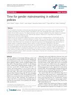
sensors. This model is w idely adopted in the oceanic prop-
agation environments as illustrated in Figure 1,whereeach
sensor receives not only the direct path signal, but reflections
from both the sea surface and the sea bottom as well [33, 34].
The primary interest of the TDE problem for this model is to
measure τ
n1
, n = 1, , N − 1, which is the TDOA between
sensor n and sensor 0 via direct path.
Jingdong Chen et al. 3
Sea surface
s[k]
w[k]
Array

Sea bottom
.
.
.
Figure 1: Illustration of the signal model in a multipath environ-
ment.
2.3. Reverberation model
The multipath model is valid for some but not all environ-
ments [35]. In addition, if there are many different paths,
that is, M is large, it is difficult to estimate all τ
nm
’s in (4).
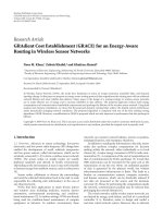
Recently, a more realistic reverberation model has been used
to describe the TDE problem in a room environment where
each sensor often receives a large number of echoes due to
reflections of the wavefront from objects and room bound-
aries such as wal ls, ceiling, and floor [15, 36, 37]. In addition,
reflections can occur several times before a signal reaches the
array, as shown in Figure 2. In this model, the received signals
are expressed as
x
n
[k] = h
n
∗ s[k]+w
n
[k], (5)
where
∗ denotes convolution, h
n

is the channel impulse re-
sponse between the source and the nth sensor, and again we
assume that s[n] is reasonably broadband and w
n
[k]isun-
correlated with s[k] and the noise signals at other sensors. In
a vector-matrix form, the signal model (5)canberewritten
as
x
n
[k] = h
T
n
s[k]+w
n
[k], n = 0, 1, , N − 1, (6)
where
h
n
=

h
n,0
h
n,1
··· h
n,L−1

T
,

s[k]
=

s[k] s[k − 1] ··· s[k − L +1]

T
,
(7)
and L is the length of the longest channel impulse responses
among N channels.
As seen, no time delay is explicitly expressed in (5), hence
there is no plain solution to the TDE problem with the rever-
beration model. In this case, TDE is often achieved in two
steps. The first step is to estimate the N channel impulse re-
sponses from the source to the N receivers. Once the chan-
nel impulse responses are measured, the TDOA information
between any two receivers is obtained by identifying the two
direct paths [15, 16, 38, 39]. Since we do not have any a priori
knowledge about the source signal and the only information
that can be accessed is the observation data, channel impulse
responses have to be estimated in a blind manner. However,
blind channel identification is a very challenging problem,
particularly in room acoustic environments where channel
impulse responses are usually ver y l ong.
s[k]
w[k]
Array
···
Figure 2: Illustration of the signal model in a reverberant environ-
ment.

3. TDE ALGORITHMS
Various TDE algorithms were developed in the literature. In
this section, we brief some critical techniques. Some of them
have already been widely used, while others may not be pop-
ular with existing systems, but have the great potential for use
in future ones.
3.1. Cross-correlation method
The cross-correlation (CC) method is the most straightfor-
ward and the earliest developed TDE algorithm, which is for-
mulated based on the single-path propagation model given
in (1) with only two receivers, that is, N
= 2. Suppose that
we have a block of observation signals at time instant k,
x
n
[k] =

x
n
[0], x
n
[1], , x
n
[l], , x
n
[K − 1]

T
=


x
n
[k], x
n
[k +1], , x
n
[k + K − 1]

T
,
(8)
where n
= 0, 1 and K is the block size, then the delay estimate
with the CC method is obtained as the lag time that maxi-
mizes the cross-correlation function (CCF) between two ob-
servation signals, that is,
τ
CC
= arg max
m
Ψ
CC
[m], (9)
where
Ψ
CC
[m] = E

x
0

[l]x
1
[l + m]

(10)
is the CCF between x
0
[l]andx
1
[l], E{·} stands for the math-
ematical expectation,
τ
CC
is an estimate of the true delay τ,
m
∈ [−τ
max
, τ
max
], and τ
max
is the maximum possible de-
lay. In digital implementation of (9), some approximations
are required because the CCF is not known and must be es-
timated. A normal practice is to replace the CCF defined in
4 EURASIP Journal on Applied Signal Processing
(10) by its time-averaged estimate, that is,

Ψ
CC

[m] =
⎧
⎪
⎪
⎪
⎪
⎪
⎪
⎪
⎨
⎪
⎪
⎪
⎪
⎪
⎪
⎪
⎩
1
K
K−m−1

l=0
x
0
[l]x
1
[l + m], m ≥ 0,
1
K

K−1

l=−m
x
0
[l]x
1
[l + m], m<0.
(11)
A similar method, formulated from the average-mag-
nitude-difference function (AMDF), was also investigated in
the literature [40], where the TDE becomes to identify the
minimum of AMDF, that is,
τ
AMDF
= arg min
m

Ψ
AMDF
[m], (12)
where

Ψ
AMDF
[m] =
⎧
⎪
⎪
⎪

⎪
⎪
⎪
⎪
⎨
⎪
⎪
⎪
⎪
⎪
⎪
⎪
⎩
1
K
K−m−1

l=0


x
0
[l] − x
1
[l + m]


, m ≥ 0,
1
K

K−1

l=−m


x
0
[l] − x
1
[l + m]


, m<0,
(13)
is the AMDF between x
0
[l]andx
1
[l]. It has been shown that
[41, 42]
E


Ψ
AMDF
[m]

=

2

π

E

x
2
0
[l]

+ E

x
2
1
[l]

− 2E


Ψ
CC
[m]

.
(14)
There are three terms in the brackets under the square root
of (14): the first two are the signal energies, and the third
is the expectation of CCF. The signal energy, which can be
treated as a constant during the observation period, does not
affect the peak position. Therefore, statistically, searching the

minimum of the AMDF is same as finding the maximum
of the CCF between two observation signals. As a result, the
AMDF approach should exhibit a similar performance to the
CC method from a statistical point of view [43].
3.2. Generalized cross-correlation method
The gener alized cross-correlation (GCC) algorithm can be
treated as an improved version of the CC method. Not only
does it unify various correlation-based algorithms into one
general framework, but it also provides a mechanism to in-
corporate knowledge to improve the performance of TDE.
This method has gained its great popularity since the land-
mark paper [5] was published by Knapp and Carter in 1976.
In this framework, the delay estimate is obtained as
τ
GCC
= arg max
m
Ψ
GCC
[m], (15)
where
Ψ
GCC
[m] =
K

−1

k


=0
Φ[k

]S
x
0
x
1
[k

]e
j2πmk

/K

=
K

−1

k

=0
σ
x
0
x
1
[k


]e
j2πmk

/K

(16)
is so-called generalized cross-correlation function (GCCF),
S
x
0
x
1
[k

] = E{X
0
[k

]X
∗
1
[k

]} is the cross-spectrum, (·)
∗
de-
notes the complex conjugate operator, X
n
[k


] is the discrete
Fourier transform (DFT) of x
n
[k], Φ[k

] is a weighting func-
tion (sometimes called a prefilter), K

is the length of the
DFT, and σ
x
0
x
1
[k

] = Φ[k

]S
x
0
x
1
[k

] is the weighted cross-
spectrum. In a practical system, the cross-spectrum S
x
0
x

1
[k

]
has to be estimated, which is normally achieved by replac-
ing the expected value by its instantaneous value, that is,

S
x
0
x
1
[k

] = X
0
[k

]X
∗
1
[k

].
There is a number of member algorithms in the GCC
family depending on how the weighting function Φ[k

]isse-
lected. Commonly used weighting functions include the con-
stant weighting (in this case, the GCC becomes a frequency-

domain implementation of the cross-correlation method
shown in (9)), the smoothed coherence transform (SCOT)
[44], the Roth processor [45], the Echart filter [5], the phase
transform (PHAT), the maximum-likelihood (ML) proces-
sor [5], the Hassab-Boucher transform [18], and so forth.
Combination of some of these functions is a lso reported in
use [46].
Different weighting functions possess different proper-
ties. For example, the PHAT algorithm uses Φ
PHAT
[k

] =
1/|S
x
0
x
1
[k

]|. Substituting Φ
PHAT
[k

] into (15) and neglecting
noise effects, one can readily deduce that the weighted cross-
spectrum is free from the source signal and depends only on
the channel responses. Consequently the PHAT algorithm
performs more consistently than many other GCC mem-
bers when the characteristics of the source signal change over

time. It is also observed that the PHAT algorithm is more im-
mune to reverberation than many other cross-correlation-
based methods. Another example is the ML processor with
which the delay estimate obtained in the ideal propagation
situation is optimal from a statistical point of view since
the estimation variance can achieve the Cram
`
er-Rao lower
bound (CRLB). It should be pointed out that in order for
the ML processor to achieve the optimal perfor mance, the
observation sample space has to be large enough; the envi-
ronments should be free of reverberation; the delay has to
be constant; and the observation signals should be station-
ary processes. In addition, the spectra of noise signals have to
be known a priori. If any of these conditions does satisfy, the
ML algorithm will then become suboptimal, like other GCC
members.
3.3. LMS-type adaptive TDE algorithm
This method, also based on the ideal propagation model
with two sensors, was proposed by Reed et al. in 1981 [26].
It has been intensively investigated in the literature since
Jingdong Chen et al. 5
then [28–30, 47]. Different from the cross-correlation-based
approaches, this algorithm achieves time delay by minimiz-
ing the mean-square error between x
0
[k]andafiltered(FIR
filter) version of x
1
[k], and the delay estimate is obtained as

the lag time associated with the largest component of the FIR
filter. If we define a signal vector of x
1
[k] at time instant k as
x
1
[k] =

x
1
[k − L], x
1
[k − L +1], , x
1
[k],
x
1
[k +1], , x
1
[k + L]

T
(17)
andanFIRfilteroflength2L +1as
h[k]
=

h
0
, h

1
, , h
l
, h
l+1
, , h
2L

T
, (18)
where L is the maximum possible time delay, then an error
signal can be formulated as
e[k]
= x
0
[k] − h
T
[k]x
1
[k]. (19)
An estimate of h[k] can be achieved by minimizing E
{e
2
[k]}
using either a batch or an adaptive algorithm. For example,
with the least-mean-square (LMS) adaptive algorithm, h[k]
can be estimated through
h[k +1]
= h[k]+μe[k]x
1

[k], (20)
where μ is a small positive adaptation step size. Given this
estimate of h[k], the delay estimate can be determined as
τ
LMS
= arg max
l


h
l


−
L. (21)
Other adaptive algorithms [48] can also be used, which may
lead to a better performance.
3.4. Fusion algorithm based on multiple sensor pairs
The GCC framework, which may yield much improvement
over the traditional direct cross-correlation method if the
weighting function is properly selected, still suffers signif-
icant performance degradation in adverse environments.
Much attention has been paid to improving the tolerance of
TDE against noise and reverberation. Besides using some a
priori knowledge about the distortion sources, another w ay
of combating noise and reverberation is through exploiting
the redundant information provided by multiple sensors. To
illustrate the redundancy, let us consider a three-sensor linear
array, which can be partitioned into three sensor pairs. Three
delay measurements can then be acquired with the observa-

tion data, that is, τ
01
(TDOA between sensor 0 and sensor 1),
τ
12
(TDOA between sensor 1 and sensor 2), and τ
02
(TDOA
between sensor 0 and sensor 2). Apparently, these three de-
lays are not independent. As a matter of fact, if the source is
located in the far field, it is easily seen that τ
02
= τ
01
+ τ
12
.
Such a relation was exploited in [49]toformulateatwo-
stage TDE algorithm. In the preprocessing stage, three delay
measurements were measured independently using the GCC
method. A state equation was then formed and a Kalman fil-
ter is used in the postprocessing stage to enhance the delay
estimate of τ
01
and τ
12
. It was shown that in the far-field case,
the estimation variance of τ
01
can be reduced by a factor of 6

in low SNR (SNR
→ 0), and of 4 in high SNR (SNR →∞)
conditions. More recently, several approaches based on mul-
tiple sensor pairs were developed to deal with TDE in room
acoustic environments [50–52]. Different from the Kalman
filter method, these approaches fuse the estimated cost func-
tions from multiple sensor pairs before searching the time
delay. We will call such a scheme as information fusion based
algorithm. In general, the problem of TDE with the fusion
algorithm can be formulated as
τ
FUSION
= arg max
m
P

p=1
F


Ψ
p
[m]

, (22)
where P is the total number of sensor pairs,

Ψ
p
[m]repre-

sents some delay cost function measured from the pth sensor
pair (it can be CCF, GCCF, AMDF, etc.), and F
{·} denotes
some mathematical transformation, which ensures that the
cost functions (

Ψ
p
[m]) for all the P sensor pairs, after trans-
formation, have their peaks due to the same source in the
same location. Various methods can be for mulated by select-
ing a different F
{·} or

Ψ. For example, if all sensor pairs are
centered around a same position, by choosing F
{x}=x,

Ψ[m] as the GCCF from the PHAT algorithm, one can read-
ily derive the so-called synchronous adding method in [50].
We can also easily derive the consistency method in [51]and
the SRP (steered response power)-PHAT algorithm in [52].
Compared with the algorithms using only two sensors, the
fusion technique can usually deliver a better per formance.
However, its computational complexity is also more than P
times of the complexity of the corresponding dual-sensor
technique, where P is the number of sensor pairs.
3.5. Multichannel cross-correlation algorithm
Recently, a squared multichannel cross-correlation coeffi-
cient (MCCC) was derived from the theory of spatial linear

prediction and interpolation [53]. Consider the signal model
given in (1) with a total of N sensors. At time instant k, the
MCCC is defined as
ρ
2
N
(k, m) = 1 −
det

R(k, m)


N−1
l
=0
r
ll
(k, m)
= 1 − det


R(k, m)

, (23)
where “det” stands for determinant of a matrix,
R(k, m) =
⎡
⎢
⎢
⎢

⎢
⎢
⎢
⎢
⎣
r
00
(k, m) r
01
(k, m) ··· r
0N−1
(k, m)
r
10
(k, m) r
11
(k, m) ··· r
1N−1
(k, m)
.
.
.
.
.
.
.
.
.
.
.

.
r
N−10
(k, m) r
N−11
(k, m) ··· r
N−1N−1
(k, m)
⎤
⎥
⎥
⎥
⎥
⎥
⎥
⎥
⎦
,
(24)
is the signal covariance matrix,
r
ij
(k, m) =
k

p=0
λ
k−p
x
i


p + f
j
(m)

x
j

p + f
i
(m)

,
i, j
= 0, 1, , N − 1,
(25)
6 EURASIP Journal on Applied Signal Processing
is the cross-correlation function between x
i
and x
j
(similar as
what is defined in (11)), λ (0 <λ
≤ 1) is a forgetting factor,

R(k, m) =
⎡
⎢
⎢
⎢

⎢
⎢
⎢
⎢
⎣
1 ρ
01
(k, m) ··· ρ
0N−1
(k, m)
ρ
10
(k, m)1··· ρ
1N−1
(k, m)
.
.
.
.
.
.
.
.
.
.
.
.
ρ
N−10
(k, m) ρ

N−11
(k, m) ··· 1
⎤
⎥
⎥
⎥
⎥
⎥
⎥
⎥
⎦
,
ρ
ij
(k, m) =
r
ij
(k, m)

r
ii
(k, m)r
jj
(k, m)
, i, j
= 0, 1, , N − 1,
(26)
is the cross-correlation coefficient between x
i
and x

j
.With
this definition, the MCCC can be estimated either in a batch
mode, which operates on a block of data snapshots [53], or in
a recursive way, which updates the estimate whenever a new
snapshot is available [54].
Just like the cross-correlation coefficient between two sig-
nals, this definition of multichannel cross-correlation co-
efficient possesses quite a few good properties, and can
be treated as a natural generalization of the traditional
cross-correlation coefficient from the two-channel to the
multichannel cases. The problem of TDE at time instant k,
based on this new definition, can be formulated a s
τ
MCCC
= arg max
m
ρ
2
N
(k, m)
= arg max
m

1 − det


R(k, m)

=

arg min
m

det


R(m, k)

.
(27)
For the particular case where we have only two receiving sen-
sors, it can be checked that
τ
MCCC
= arg max
m
ρ
2
N
(k, m)
= arg max
m
ρ
2
01
(k, m),
(28)
which is same as the cross-correlation method shown in
Section 3.1. When we have more than two sensors, this
method can be v iewed as a natural generalization of the

cross-correlation method to the multichannel case, which
can take advantage of the redundancy among multiple sen-
sors to improve the time delay estimate between two sensors.
It is worth mentioning that a prewhitening process can be
applied to the observation signals before delay estimation. In
this case, the MCCC algorithm can be treated as a generalized
version of the PHAT algorithm.
3.6. Adaptive eigenvalue decomposition algorithm
All the algorithms outlined in the previous sections achieve
delay estimate by measuring the cross-correlation between
two or among multiple channels. A common assumption
with these methods is that each sensor receives only the
direct-path signal. Recently, an adaptive eigenvalue decom-
position (AED) algorithm was proposed to deal with TDE
in room reverberant environment [15, 55]. Unlike the cross-
correlation-based methods, this algorithm first identifies the
channel impulse responses from the source to the two s en-
sors. The delay estimate is then determined by finding the
direct paths from the two measured impulse responses. Ap-
parently, this algorithm takes fully into account the reverber-
ation effect during time delay estimation.
For the signal model given in (5) with two sensors, if the
noise term is neglected, one can easily check that
x
0
[k] ∗ h
1
= s[k] ∗ h
0
∗ h

1
= x
1
[k] ∗ h
0
. (29)
At time instant k, this relation can be rewritten in a vector-
matrix form as [15]
x
T
[k]u = x
T
0
[k]h
1
− x
T
1
[k]h
0
= 0, (30)
where
x
n
[k] =

x
n
[k] x
n

[k − 1] ··· x
n
[k − L +1]

T
,
x[k]
=

x
T
0
[k] x
T
1
[k]

T
,
u
=

h
T
1
−h
T
0

T

,
(31)
and n
= 0, 1. Left multiplying ( 30)byx[n] and taking expec-
tation yields
Ru
= 0, (32)
where R
= E{x [k]x
T
[k]} is the covariance matrix of the sen-
sor signals. This implies that vector u which consists of two
impulse responses is in the null space of R.Morespecifically,
u is the eigenvector of R corresponding to the eigenvalue 0. It
has been shown that the two channel impulse responses (i.e.,
h
0
and h
1
) can be uniquely determined (up to a scale and
a common delay) from (32) if the following two conditions
hold [56–58]:
(i) the polynomials formed from h
0
and h
1
(i.e., the Z-
transforms of h
0
and h

1
) are coprime, or they do not
share any common zeros;
(ii) the autocorrelation matrix of the source signal s[k],
that is, R
ss
= E{s[k]s
T
[k]}, is of full rank.
See [56, 59] for a detailed description about the necessary
and sufficient conditions for the identifiability. Note that the
scale and common-delay ambiguities of blind identification
techniques does not affect the problem of TDE.
When an independent white noise signal is present on
each sensor, it will regularize the covariance matrix; as a con-
sequence, R does not have a zero eigenvalue anymore. In such
a case, an estimate of the impulse responses can be achieved
through the following algorithm, which is an adaptive way to
find the eigenvector associated with the smallest eigenvalue
Jingdong Chen et al. 7
of R [15]:
u[k +1]=

u[k] − μe[k] x[k]



u[k] − μe[k] x[k]



, (33)
with the constraint that
u[k]=1, where
e[k]
= u
T
[k]x[k] (34)
is an error signal,
·denotes the l
2
norm of a vector or
matrix, and μ, the adaptation step, is a positive constant.
With the identified impulse responses

h
0
and

h
1
, the time
delay estimate is determined as the difference between two
direct paths, that is,
τ
AED
= arg max
l




h
1,l


−
arg max
l



h
0,l


. (35)
3.7. Adaptive multichannel time delay estimation
In the AED algorithm, the delay estimate is obtained by
blindly identifying two channel impulse responses. It re-
quires that the two channels do not share any common ze-
ros, which is usually true for systems with short impulse re-
sponses. In many application scenarios such as room acoustic
environments, however, the channel impulse response from
the source to the microphone sensor could be very long, de-
pending on the reverberation condition. As the length of the
two impulse responses becomes longer, the probability for
them not sharing common zeros will become lower and the
AED algorithm often fails when a zero is shared between two
channels or some zeros of the two channels are close. One
way to overcome this problem is to employ more channels
in the system, since it would be less likely for all channels to

share a common zero when the number of sensors is large.
This idea leads to an adaptive multichannel (AMC) time de-
lay estimation approach based on a blind channel identifica-
tion technique [39 ].
Considering the reverberation model in (5), we can de-
fine a cost function among all the N channels, at time instant
k +1,as
J[k +1]
=
N−2

i=0
N
−1

j=i+1
e
2
ij
[k + 1], (36)
where
e
ij
[k +1]=
x
T
i
[k +1]

h

j
[k] − x
T
j
[k +1]

h
i
[k]



h[k]


,
i, j
= 0, 1, , N − 1,
(37)
is an error signal between sensor i and sensor j at time k +1,

h
n
[k] is the modeling filter of h
n
[k], and

h[k] =



h
T
0
[k]

h
T
1
[k] ···

h
T
N
−1
[k]

T
. (38)
It follows immediately that various adaptive algorithms can
be used to achieve an estimate of

h[k], by minimizing J[k+1].
For example, a multichannel LMS (MCLMS) algorithm was
derived in [60], which updates

h through

h[k +1]=

h[k] − 2μ



R[k +1]

h[k] − J[k +1]

h[k]




h[k] − 2μ


R[k +1]

h[k] − J[k +1]

h[k]



,
(39)
where again μ, the adaptation step, is a positive constant,

R[k +1]=
⎡
⎢
⎢

⎢
⎢
⎢
⎢
⎢
⎢
⎢
⎢
⎢
⎣

i=0

R
x
i
x
i
[k+1] −

R
x
1
x
0
[k+1] ··· −

R
x
N−1

x
0
[k+1]
−

R
x
0
x
1
[k+1]

i=1

R
x
i
x
i
[k+1] ··· −

R
x
N−1
x
1
[k+1]
.
.
.

.
.
.
.
.
.
.
.
.
−

R
x
0
x
N−1
[k+1] −

R
x
1
x
N−1
[k+1] ···

i=N−1

R
x
i

x
i
[k+1]
⎤
⎥
⎥
⎥
⎥
⎥
⎥
⎥
⎥
⎥
⎥
⎥
⎦
,

R
x
i
x
j
[k +1]= x
i
[k +1]x
T
j
[k +1], i, j = 0, 1, , N − 1.
(40)

It was shown that with this MCLMS algorithm the channel
estimate can converge in mean to the true impulse responses
(up to a scale and common delay). However, the convergence
rate of this algorithm is normally slow. To accelerate the con-
vergence rate, a normalized multichannel frequency-domain
LMS (NMCFLMS) algorithm was developed in [25]. Dif-
ferent from the MCLMS method, which updates the chan-
nel estimate every snapshot, the (NMCFLMS) algorithm op-
erates in the frequency domain on a block-by-block basis.
First, the multichannel observation signals are partitioned
into successive blocks. The fast Fourier transform (FFT) is
then applied to each block to estimate its Fourier spectrum.
The frequency-domain channel estimate is then updated us-
ing the normalized LMS algorithm. Finally, the time-domain
impulse responses are obtained by applying the inverse FFT
to the frequency-domain channel estimate. See Algorithm 5
for how to obtain the channel estimates and [25] for the de-
tailed derivation of the NMCFLMS algorithm.
Once

h[k] is a chieved (with either the MCLMS algorithm
or the NMCFLMS algorithm), the time-domain estimate of
impulse responses is obtained by the inverse Fourier trans-
form, and time delay between the ith and jth sensors is de-
termined as
τ
ij
= arg max
l




h
j,l


−
arg max
l



h
i,l


. (41)
4. ALGORITHM COMPLEXITY
This section briefly compares the computational complexity
of different TDE algorithms. As seen, all the algorithms esti-
mate time-delay information in two steps. The first step in-
volves the estimation of the cost function. The second step
obtains time delay estimate by searching the extremum of
the cost function. If we assume that different cost functions
have the same length, it can be easily checked that all the
8 EURASIP Journal on Applied Signal Processing
Algorithm step: (Real-valued) multiplications:
Obtain a frame of observation signal at time instant k:
x
n

[k] =

x
n
[0], x
n
[1], , x
n
[K − 1]

T
=

x
n
[k], x
n
[k +1], , x
n
[k + K − 1]

T
Estimate the spectrum of x
0
[k]:
X
0
[k

] =

K−1

k=0
x
0
[k]e
− j2πkk

/K
K
2
log
2
(K) −
5K
4
= FFT
K

x
0
[k]

,(k

= 0, 1, , K

− 1)
Estimate the spectrum of x
1

[k]:
X
1
[k

] =
K−1

k=0
x
1
[k]e
− j2πkk

/K
K
2
log
2
(K) −
5K
4
= FFT
K

x
1
[k]

,(k


= 0, 1, , K

− 1)
Compute the weighted cross-spectrum:
S
x
0
x
1
[k

]


S
x
0
x
1
[k

]


=
E

X
0

[k

]X
∗
1
[k

]



E

X
0
[k

]X
∗
1
[k

]



4K +8
Estimate the PHAT cost function:

Ψ

PHAT
[m] =
K

−1

k

=0
S
x
0
x
1
[k

]


S
x
0
x
1
[k

]


e

j2πmk

/K

2K log
2
(K) − 7K +12
= FFT
−1
K

S
x
0
x
1
[k

]


S
x
0
x
1
[k

]




,(m = 0, 1, , K − 1)
Tot al : 3K log
2
K −
11
2
K +20
Total/sample: 3 log
2
K −
11
2
+
20
K
Algorithm 1: Computational complexity of the PHAT algorithm. FFT
K
{·} and IFFT
−1
K
{·} are K-point fast Fourier and inverse fast Fourier
transforms, respectively. In addition, due to the symmetric property, we only need to perform K/2 + 1 complex multiplications and divisions
during computation of the weighted spectrum.
algorithms have a similar complexity in the second step.
Therefore, we only compare the computational burdens re-
quired for estimating the cost function. Here the com-
putational complexity is evaluated in terms of the num-
ber of real-valued multiplications/divisions required for the

implementation of each algorithm. The number of ad-
ditions/subtractions are neglected because they are much
quicker to compute in most generic hardware platforms. We
assume that complex-valued multiplications are transformed
into real-valued multiplications. The multiplication between
a real number and complex number requires 2 real-valued
multiplications. The multiplication between two complex
numbers needs 4 real-valued multiplications. The division
between a complex number and a real number requires 2
real-valued multiplications.
As mentioned earlier, there are different member algo-
rithms in the GCC family. Each involves two FFT opera-
tions to estimate the cross-spectrum, some multiplications
for the weighting process, and an IFFT operation for com-
puting the GCC function. If the Fourier transform of a real-
valued series of length K is computed using the FFT rou-
tine devised by [61], it requires (K/2) log
2
(K) − 5K/4mul-
tiplications. An IFFT operation of a complex-valued series
of length K requires 2K log
2
(K) − 7K + 12. The complex-
ity of the PHAT algorithm is summarized in Algorithm 1.
Similarly, the computational load for other GCC member
algorithms can be easily counted, which will not be presented
here.
Unlike the GCC method, which estimates the time de-
lay on a frame-by-frame basis, the LMS-type adaptive al-
gorithm updates the cost function whenever a new data

sample is available. For each data sample, the number of
multiplications required for computing the cost function is
shown in Algorithm 2, which is higher than that of the PHAT
algorithm.
The MCCC can be computed either on a block-by-block
basis or in an iterative way. Its complexity is described in
Algorithm 3. We see that, depending on the number of sen-
sors, the MCCC algorithm is generally more computationaly
expensive than the GCC method. Notice that more compu-
tationally efficient algorithm can be formulated to calculate
MCCC using FFT. This is, however, beyond the scope of this
paper.
The computational burdens required for the estimation
of channel impulse responses using either the AED or the
NMCFLMS algorithms are presented in Algorithms 4 and 5,
respectively. Depending on the length of the modeling filter,
the estimation of channel impulse responses usually requires
more multiplications than estimating the gener alizing cross-
correlation function. However, such a magnitude of compu-
tational complexity should not be a big concern with today’s
computer processors.
Jingdong Chen et al. 9
Algorithm step: (Real-valued) multiplications:
Parameters:
h[k]
=

h
0
, h

1
, , h
l
, h
l+1
, , h
2L

T
Obtain a signal vector x
1
at time instant k:
x
1
[k] =

x
1
[k − L], x
1
[k − L +1], , x
1
[k − 1],
x
1
[k], x
1
[k +1], , x
1
[k + L]


T
Compute the error signal at time instant k:
e[k]
= x
0
[k] − h
T
[k]x
1
[k]2L +1
Update the filter coefficients:
h[k +1]
= h[k]+μe[k]x
1
[k]2L +2
Total/sample: 4L +3
Algorithm 2: Computational complexity of the LMS-type adaptive algorithm.
Algorithm step: (Real-valued) multiplications:
Obtain a frame of observation signal at time instant k:
x
n
[k], k = 0, 1, , K − 1,
n
= 0, 1, , N − 1
Prewhitening:
x

n
[k] = IFFT

K

FFT
K

x
n
[k]

/


FFT
K

x
n
[k]




, N

5
2
K log
2
(K) −
31

4
K +13

n = 0, 1, , N − 1
Compute matrix

R(k, m):

R(k, m) =
⎡
⎢
⎢
⎢
⎢
⎣
1 ρ
01
(k, m) ··· ρ
0N−1
(k, m)
ρ
10
(k, m)1··· ρ
1N−1
(k, m)
.
.
.
.
.

.
.
.
.
.
.
.
ρ
N−10
(k, m) ρ
N−11
(k, m) ··· 1
⎤
⎥
⎥
⎥
⎥
⎦
(2K +3)N(N − 1)

2τ
max
+1

ρ
ij
(k, m) =
r
ij
(k, m)


r
ii
(k, m)r
jj
(k, m)
r
ij
(k, m) = λr
ij
(k − 1, m)+x
i
[p + m]x
j
[p + m]
i, j
= 0, 1, , N − 1
−τ
max
≤ m ≤ τ
max
Estimate the MCCC cost function:
det


R(k, m)

, −τ
max
≤ m ≤ τ

max

2τ
max
+1


N
3
3
+
5N
3

Tot al : 4τ
max
KN
2
+4τ
max
KN +2KN
2
+
5
4
NK +
5
2
NK log
2

K +
2
3
τ
max
N
3
+6τ
max
N
2
+
1
3
N
3
+
28
3
τ
max
N +3N
2
+
43
3
N
Total/sample: 4τ
max
N

2
+4τ
max
N +2N
2
+
5
4
N +
5
2
N log
2
K
+
1
K

2
3
τ
max
N
3
+6τ
max
N
2
+
1

3
N
3
+
28
3
τ
max
N +3N
2
+
43
3
N

Algorithm 3: Computational complexity of the MCCC algorithm. It is assumed that determinant of a matri x is computed through LU
decomposition, which requires N
3
/3+5N/3 multiplications [62].
5. RESOLUTION PROBLEM
All the TDE techniques described above measure time de-
lay based on discrete signal samples. The delay estimate is,
therefore, an integral multiple of the sampling period. Such a
resolution, depending on the sampling rate and several other
factors, may not be adequate for some applications. How to
improve the TDE resolution becomes another challenging
problem, and has attracted much attention in the past few
decades. Different solutions can be applied, depending on
10 EURASIP Journal on Applied Signal Processing
Algorithm step: (Real-valued) multiplications:

Parameters:
u
=

h
T
1
−h
T
0

T
,
h
0
=

h
0,0
h
0,1
··· h
0,L−1

T
,
h
1
=


h
1,0
h
1,1
··· h
1,L−1

T
Construct the signal vector at time instant k:
x[k]
=

x
T
0
[k] x
T
1
[k]

T
,
x
0
[k] =

x
0
[k], x
0

[k − 1], , x
0
[k − L +1]

T
x
1
[k] =

x
1
[k], x
1
[k − 1], , x
1
[k − L +1]

T
Compute the error signal at time instant k:
e[k]
=

u
T
[k]x[k]2L
Update the filter coefficients:
u[k +1]=

u[k] − μe[k]x[k]




u[k] − μe[k]x[k]


,6L +2
Total/sample: 8L +2
Algorithm 4: Computational complexity of the AED algorithm.
the TDE algorithm and the nature of application. To illus-
trate, let us examine a simple case in the context of direction
of arrival (DOA) estimation, where we have two sensors and
one source in the far field as shown in Figure 3. The angular
resolution, which governs the ability of the system to sepa-
rate two closely spaced sources, is determined by how many
different DOA measurements can be made between 0 and π.
Assuming that the distance between two sensors is d, the ve-
locity of wave propagation is c, and the sampling rate is f ,
we can easily check that the maximum τ in samples that can
be estimated is df/c, the minimal τ is −df /c, and the bearing
angle θ relates to the time delay τ by
θ
= arccos
cτ
d
. (42)
Therefore, the number of different measurements of θ in
[0, π] depends on the number of different delay estimates in
[
−df/c, df /c]. As a result, to increase the angular resolution,
we need to have more different delay measurements between

−df/c and df/c. This can be achieved through the following
three ways.
(i) Interpolation. Since its mathematical expectation is
shown to be band limited and present a symmetric
peak around the true time delay, the estimated cross-
correlation function can be approximated by a con-
cave parabola in the neighbor hood of its maximum
[40, 63, 64]. As a result, parabolic inter polation can
be applied to the cross-correlation-based algorithms
to obtain a finer TDE resolution, which is a frac-
tion of the sampling period. Such a scheme has been
adopted in many systems. However, if the statistic of
the cost function is not band limited, we, in general,
cannot apply parabolic interpolation. Note that in real
environments, the applicability of interpolation is also
limited by the SNR condition. If the SNR is very low,
then interpolation will introduce significant bias. For
the channel identification TDE techniques, if the es-
timated channel impulse responses approximate the
true ones, interpolation technique can also be applied
to increase resolution. However, in most situations,
the impulse responses estimated with the blind tech-
niques are only accurate enough for identifying the di-
rect path, but not good enough for interpolation.
(ii) Increasing the sampling rate. The higher the sampling
rate, the more the number of different delay estimates
can be acquired between
−df/c and df /c,whichinturn
leads to a higher DOA resolution. This approach, how-
ever, will increase the complexity of both the TDE a l-

gorithm and some subsequent processing blocks of the
system.
(iii) Increasing d. DOA resolution can also be improved
by increasing d. Apparently, this will increase the ar-
ray size. Therefore this method is hard to implement
in scenarios where the space is limited. Also, a larger d
may cause spatial aliasing problem, which may not be a
big concern for the task of source localization, but has
to be treated with great care in the context of beam-
forming and noise reduction. In addition, increasing
d may lead to a higher complexity since we may have
to increase the block size to compute the cost function
and search the delay estimates in a larger delay range.
6. EXPERIMENTS
This section attempts to compare the performance of differ-
ent TDE algorithms in both noisy and reverberant environ-
ments.
Jingdong Chen et al. 11
Algorithm step: (Real-valued) multiplications:
Parameters:
h
=

h
T
0
h
T
1
··· h

T
N
−1

T
, h
n
=

h
n,0
h
n,1
··· h
n,L−1

T
,
μ
f
, the step size; δ, the regularization factor
Initialization:
h
n
[0] and p
n
[0],
Construct a frame of signal of length 2L at time instant k;
Update Filter coefficients at time k (for k
= 0, 1, ):

h
10
n
[k] = FFT
2L

h
T
n
[k] 0
1×L

T

; N

L log
2
(L) −
3
2
L

x
n
[k +1]
2L×1
= FFT
2L


x
n
[k +1]
2L×1

; N

L log
2
(L) −
3
2
L

p
n
[k +1]= λp
n
[k]
2L×1
+(1− λ)
N−1

i=0, i=k
x
∗
i
[k +1] x
i
[k +1]; 4N

2
L − 2NL

p
n
[k +1]+δ1
2L×1

−→
p
−1
n
[k +1]
2L×1
;2NL
e
ij
[k +1]
2L×1
=
⎧
⎨
⎩
x
i
[k +1] h
10
j
[k] − x
j

[k +1] h
10
i
[k], i = j
0
2L×1
, i = j
2N
2
L − 2NL
(i, j
= 0, 1, , N − 1)
e
ij
[k +1]
2L×1
= IFFT
2L


e
ij
[k +1]
2L×1

;
N(N
− 1)
2


L log
2
L −
3
2
L

Obtain e
ij
[k + 1], which consists of the last L elements of e
ij
[k +1];
e
01
ij
[k +1]= FFT
2L

0
1×L
e
T
ij
[k +1]

T

;
N(N
− 1)

2

L log
2
L −
3
2
L

Δh
10
n
[k] =
N−1

i=0
x
∗
i
[k +1] e
01
in
[k +1] p
−1
n
[k +1], 4NL
Δh
10
n
[k] = IFFT

2L

Δh
10
n
[k]

, N

L log
2
L −
3
2
L

h
10
n
[k +1]= h
10
n
[k] − μ
f
Δh
10
n
[k], 2NL
Obtain h
n

[k +1]
L×1
, which consists of the first L elements of h
10
n
[k +1]
2L×1
.
h[k +1]
=
h[k +1]


h[k +1]


(impose the unit-norm constraint) NL
Tot al : N(N +2)

L log
2
L −
3
2
L

+5NL+6N
2
L
Total/sample: N(N +2)


log
2
L −
3
2

+6N
2
+5N
Algorithm 5: Computational complexity of the NMCFLMS algorithm. FFT
2L
{·} and IFFT
2L
{·} are 2L-point fast Fourier and inverse fast
Fourier transforms, respectively.
 denotes dot product.
6.1. Experimental setup
In an attempt to simulate reverberant acoustic environments,
the image model technology [65] is used. We consider a
rectangular room with plane reflective boundaries (walls,
ceiling, and floor). Each boundary is characterized by a uni-
form reflection coefficient, which is independent of the fre-
quency and the incidence angle of the source signal. The fol-
lowing parameter values are used.
(i) Room dimensions: 120
× 180 × 150 inch (x × y × z).
(ii) Reflection coefficients: r
i
(i = 1, 2, , 6) varying be-

tween 0 and 1.
(iii) Source position: two point omnidirectional sources
are located at (100, 100, 40) and (32, 100, 40), respec-
tively.
(iv) Sensor positions: a linear array which consists of four
(4) ideal point microphones placed in parallel with the
x-axis. The four microphones are located at (20, 10,
40), (28, 10, 40), (36, 10, 40), and (44, 10, 40), respec-
tively. The directivity pattern of each microphone is as-
sumed to be omnidirectional.
(v) SNR: varying between
−10 dB and 25 dB.
A low-pass sampled version of the impulse response of
the acoustic transmission channel between each source and
12 EURASIP Journal on Applied Signal Processing
Table 1: Parameter setup for each TDE algorithm.
Window size Window type FFT size Smoothing factor Filter length Adaptation step size
CC K = 1024 Kaiser K

= 1024 γ = 0.95 N/A N/A
PHAT K
= 1024 Kaiser K

= 1024 γ = 0.95 N/A N/A
ML K
= 1024 Kaiser K

= 1024 γ = 0.95 N/A N/A
AED K
= 1024 Rectangular N/A γ = 0.95 L = 1024 μ = 0.01

LMS N/A N/A N/A N/A L
= 1024 μ = 0.0001
MCCC K
= 1024 Rectangular N/A γ = 0.95 N/A N/A
AMC K
= 1024 Rectangular 2048 λ = 0.8[60] L = 1024 μ
f
= 0.2[60]
FUSION K
= 1024 Kaiser K

= 1024 γ = 0.95 N/A N/A
s[k]
Plane wavefront
θ
d
Sensor 1 Sensor 0
Figure 3: Illustration of TDE resolution problem in the context of DOA estimation.
each microphone is generated using the image method. A
speech signal from a female speaker, digitized with 16-bit res-
olution at 16 kHz, is then convolved with the synthetic im-
pulse responses. Finally, mutually independent white Gaus-
sian noise is properly scaled and added to each microphone
signal to control the SNR.
6.2. Implementation
Delay estimates were obtained on a frame-by-frame basis.
The frame size used in all experiments is 64 ms. For the cross-
correlation-based techniques (including dual- and multiple-
channel algorithms), a 64-ms Kaiser window was applied to
the analysis frame, while a rectangular window of the same

length was applied for the channel identification-based algo-
rithms. To reduce the temporal effect of noise on TDE per-
formance, the cost function of each algorithm is smoothed
using a single-pole recursion as follows:
¯
Ψ
k
= γ
¯
Ψ
k−1
+(1− γ)

Ψ
k
, (43)
where

Ψ
k
denotes the cost func tion estimated using the kth
frame of observation data,
¯
Ψ
k
is a smoothed version of the
cost function, based on which the delay estimates were ob-
tained. For the MCCC algorithm, the signal was prewhitened
before computing the cost function. Therefore, this method,
in the case of two sensors, is equivalent to the PHAT algo-

rithm. For the ML method, we assume that the noise spec-
trum is known a priori. The fusion algorithm implemented
here is the consistency method presented in [51]. All the pa-
rameters used in each algorithm are summarized in Table 1.
It is not always easy to compare fairly different algo-
rithms. In our experiments, we optimized each individual
algorithm in a nonreverberant and weak noisy (SNR
=
25 dB) environment to its best performance. We then test
and compare all the algorithms in reverberation and differ-
ent noise conditions. Such a process should, in generally, not
favor any specific algorithm.
6.3. Experimental results
A great deal of efforts have been devoted to analyzing the
TDE performance of the GCC technique in reverberant envi-
ronments [66, 67]; but not much comparison has been made
between correlation and system-identification-based algo-
rithms. In this experiment, we compare all the algorithms
Jingdong Chen et al. 13
0
20
40
60
80
100
Percent hits
−10 −6
−22 610
Delay (samples)
T

60
= 120 ms
CC:
0
20
40
60
80
100
Percent hits
−10 −6
−22 610
Delay (samples)
T
60
= 350 ms
0
20
40
60
80
100
Percent hits
−10 −6
−22 610
Delay (samples)
T
60
= 580 ms
0

20
40
60
80
100
Percent hits
−10 −6
−22 610
Delay (samples)
PHAT:
0
20
40
60
80
100
Percent hits
−10 −6
−22 610
Delay (samples)
0
20
40
60
80
100
Percent hits
−10 −6
−22 610
Delay (samples)

0
20
40
60
80
100
Percent hits
−10 −6
−22 610
Delay (samples)
ML:
0
20
40
60
80
100
Percent hits
−10 −6
−22 610
Delay (samples)
0
20
40
60
80
100
Percent hits
−10 −6
−22 610

Delay (samples)
0
20
40
60
80
100
Percent hits
−10 −6
−22 610
Delay (samples)
AED:
0
20
40
60
80
100
Percent hits
−10 −6
−22 610
Delay (samples)
0
20
40
60
80
100
Percent hits
−10 −6

−22 610
Delay (samples)
0
20
40
60
80
100
Percent hits
−10 −6
−22 610
Delay (samples)
LMS:
0
20
40
60
80
100
Percent hits
−10 −6
−22 610
Delay (samples)
0
20
40
60
80
100
Percent hits

−10 −6
−22 610
Delay (samples)
0
20
40
60
80
100
Percent hits
−10 −6
−22 610
Delay (samples)
MCCC:
0
20
40
60
80
100
Percent hits
−10 −6
−22 610
Delay (samples)
0
20
40
60
80
100

Percent hits
−10 −6
−22 610
Delay (samples)
0
20
40
60
80
100
Percent hits
−10 −6
−22 610
Delay (samples)
AMC:
0
20
40
60
80
100
Percent hits
−10 −6
−22 610
Delay (samples)
0
20
40
60
80

100
Percent hits
−10 −6
−22 610
Delay (samples)
0
20
40
60
80
100
Percent hits
−10 −6
−22 610
Delay (samples)
FUSION:
0
20
40
60
80
100
Percent hits
−10 −6
−22 610
Delay (samples)
0
20
40
60

80
100
Percent hits
−10 −6
−22 610
Delay (samples)
Figure 4: TDE performances in moderate noisy and reverberant environments, where SNR = 15 dB and T
60
= 120 ms, 350 ms, and 580 ms,
respectively.
14 EURASIP Journal on Applied Signal Processing
outlined previously for their performances in different re-
verberant environments. Figure 4 shows histograms of TDE
in a moderate noise condition where SNR
= 15 dB. The
source is a speech signal from a female speaker and its loca-
tion is in (100, 100, 40). The first, second, and third columns
correspond, respectively, to reverberation times of 120 ms,
350 ms, and 580 ms. The true time delay between sensor 0
and 1 is equal to 5 (samples). It can be seen that, in the
first two reverberant environments, all algorithms can accu-
rately identify the time delay. When reverber ation time is in-
creased to 580 ms, both the CC and the ML methods suffer
significant performance degradation, showing that these two
approaches are sensitive to reverber ation. The PHAT algo-
rithm, though also belongs to the GCC family like the CC
and ML methods, still yields a reasonable performance, im-
plying its robustness with respect to reverberation. This cor-
roborates with many observations reported in the literature
[46]. Among the five techniques that use two sensors (i.e.,

CC, PHAT, ML, AED, LMS), the AED algorithm delivers the
best performance. This indicates that taking it into a ccount
in the sig nal model is an effective way in dealing with re-
verberation. Comparing the MCCC, AMC, and fusion algo-
rithms with dual-sensor techniques, one can easily see the
advantage of using multiple sensors. Since the AMC algo-
rithm was formulated from the reverberation signal model
and using multiple sensors, it is not surprising to see that it
achieves the best performance in this strong reverberant en-
vironment.
The second experiment involves a set of data obtained in
nonreverberant (simulated by setting all the reflection coef-
ficients to 0) but noisy environments. The source signal and
its presentation are the same as in the previous experiment.
Figure 5 shows histograms of delay estimates. The first, sec-
ond, and third columns correspond, respectively, to noise
conditions of SNR
= 15 dB, 5 dB, and −5 dB. In general, all
TDE techniques are quite robust to noise. They work pretty
well even when SNR is as low as 5 dB. When SNR drops
down to
−5 dB, the TDE performance begin to deteriorate,
even though the degree of degradation may vary across al-
gorithms. Among all the eight algorithms studied, the LMS
method is most sensitive to noise. We may consider to im-
prove this technique by using some adaptive algorithms that
have a faster convergence rate or a low steady-state error.
The PHAT algorithm, which demonstrated the highest ro-
bustness with respect to reverberation in the GCC family, is
inferior to b oth the CC and the ML approaches in additive

noise. The ML algorithm delivers a better performance than
the CC method. This indicates that some a priori knowledge
can help the estimator to cope with distortion. Among the
five dual-sensor techniques, we noticed that the AED algo-
rithm demonstrates the highest robustness not only to re-
verberation, but to additive noise as well. This observation
is different from our intuition since it is well perceived that
the blind channel identification technique is in general sen-
sitive to noise. We attribute this to the nature of the TDE
problem, which only requires to identify the direct path. Es-
timation of the whole impulse response, depending on its
length and many other factors, may be sensitive to noise; but
identification of the direct path is a much easier task, and it
canbeimmunetonoise.
Comparing the AMC with the AED algorithm, we did
not see much improvement as we observed in the previous
experiment. This is understandable. The motivation behind
the AMC algorithm is to circumvent the common-zero prob-
lem. The probability of a common zero shared among chan-
nels decreases when the number of channels increases. How-
ever, in this experiment, al l the channels apparently share no
common zero since there is no reverberation. As a result, the
AMC is similar to the AED algorithm in performance.
Both the MCCC and fusion methods yield a performance
superior to that of the techniques with two sensors, indicat-
ing that using multiple sensors is a good way to improve the
robustness of TDE with respect to additive noise. The MCCC
shows a better performance than the fusion method.
The final experiment is to test the TDE algorithms for
their t racking ability. To simulate a moving source, we first

place the source at (100, 100, 40) for 30 seconds, and then
switch to (32, 100, 40). Again, the source is a speech signal
as used in the previous experiments. In this case, the true
delay in the first 30 seconds is 5 (samples), and 3 (samples)
then. The average SNR is 0 dB, and T
60
= 240 ms. Figure 6
shows the TDE results. The AED, LMS, and AMC algorithms
are adaptive in nature. They take some time to converge to a
new delay. All other five methods are nonadaptive. However,
due to the smoothing processing, they also take some time to
adapt to the new source position. From the results, one can
see that all the algorithms can adjust to the new delay in less
than one second.
7. SUMMARY
Time delay estimation, which serves as a fundamental step
for a source localization or a beamforming system, has at-
tracted a considerable amount of research attention in the
past few decades. Various techniques were developed in
the literature. This paper briefly summarized these efforts,
and reviewed the state of the art, the critical techniques,
and the recent advances which had significantly improved
performance of time delay estimation in adverse environ-
ments. Broadly, the reviewed techniques can be classified into
two categories: cross-correlation-based methods and system
identification-based approaches. Both categories can be im-
plemented either based on two sensors, or using multiple
sensors. We evaluated eight algorithms, including five dual-
channel techniques and three multiple-channel techniques,
in both reverberant and noisy environments. Among the five

studied dual-channel techniques, the adaptive eigenvalue de-
composition algorithm demonst rated the best performance
in both noise and reverberation conditions, showing its great
potential for real applications. In general, more sensors will
lead to a higher robustness because of the redundancy. How-
ever, it should be pointed out that attention has to be paid to
implementing the multichannel cross-correlation algorithm
and the fusion method. Both need to synchronize either the
signals observed at different sensors, or the cost functions
from different sensor pairs. In case that the true delay is not
Jingdong Chen et al. 15
0
20
40
60
80
100
Percent hits
−10 −6
−22 610
Delay (samples)
SNR
= 15 dB
CC:
0
20
40
60
80
100

Percent hits
−10 −6
−22 610
Delay (samples)
SNR
= 5dB
0
20
40
60
80
100
Percent hits
−10 −6
−22 610
Delay (samples)
SNR
=−5dB
0
20
40
60
80
100
Percent hits
−10 −6
−22 610
Delay (samples)
PHAT:
0

20
40
60
80
100
Percent hits
−10 −6
−22 610
Delay (samples)
0
20
40
60
80
100
Percent hits
−10 −6
−22 610
Delay (samples)
0
20
40
60
80
100
Percent hits
−10 −6
−22 610
Delay (samples)
ML:

0
20
40
60
80
100
Percent hits
−10 −6
−22 610
Delay (samples)
0
20
40
60
80
100
Percent hits
−10 −6
−22 610
Delay (samples)
0
20
40
60
80
100
Percent hits
−10 −6
−22 610
Delay (samples)

AED:
0
20
40
60
80
100
Percent hits
−10 −6
−22 610
Delay (samples)
0
20
40
60
80
100
Percent hits
−10 −6
−22 610
Delay (samples)
0
20
40
60
80
100
Percent hits
−10 −6
−22 610

Delay (samples)
LMS:
0
20
40
60
80
100
Percent hits
−10 −6
−22 610
Delay (samples)
0
20
40
60
80
100
Percent hits
−10 −6
−22 610
Delay (samples)
0
20
40
60
80
100
Percent hits
−10 −6

−22 610
Delay (samples)
MCCC:
0
20
40
60
80
100
Percent hits
−10 −6
−22 610
Delay (samples)
0
20
40
60
80
100
Percent hits
−10 −6
−22 610
Delay (samples)
0
20
40
60
80
100
Percent hits

−10 −6
−22 610
Delay (samples)
AMC:
0
20
40
60
80
100
Percent hits
−10 −6
−22 610
Delay (samples)
0
20
40
60
80
100
Percent hits
−10 −6
−22 610
Delay (samples)
0
20
40
60
80
100

Percent hits
−10 −6
−22 610
Delay (samples)
FUSION:
0
20
40
60
80
100
Percent hits
−10 −6
−22 610
Delay (samples)
0
20
40
60
80
100
Percent hits
−10 −6
−22 610
Delay (samples)
Figure 5: TDE performances in nonreverberant but noisy environments, where SNR = 15 dB, 5 dB, and −5dB,respectively.
16 EURASIP Journal on Applied Signal Processing
−10
−5
0

5
10
Delay (samples)
0102030405060
Time (s)
CC
−10
−5
0
5
10
Delay (samples)
0102030405060
Time (s)
PHAT
−10
−5
0
5
10
Delay (samples)
0102030405060
Time (s)
ML
−10
−5
0
5
10
Delay (samples)

0102030405060
Time (s)
AED
−10
−5
0
5
10
Delay (samples)
0102030405060
Time (s)
LMS
−10
−5
0
5
10
Delay (samples)
0102030405060
Time (s)
MCCC
−10
−5
0
5
10
Delay (samples)
0102030405060
Time (s)
AMC

−10
−5
0
5
10
Delay (samples)
0102030405060
Time (s)
FUSION
Figure 6: Tracking performance of different algorithms in a noisy and reverberant environment, where SNR = 0dBandT
60
= 240 ms.
Jingdong Chen et al. 17
the integral multiple of the sampling rate, we wil l have to ei-
ther increase the sampling rate or use interpolation, which
may significantly increase the computational complexity. In
case that the observation signals or the cost functions are not
properly aligned, we may not achieve much improvement.
REFERENCES
[1] J. E. Ehrenberg, T. E. Ewart, and R. D. Morris, “Signal-
processing techniques for resolving individual pulses in a mul-
tipath signal,” Journal of the Acoustical Society of America,
vol. 63, no. 6, pp. 1861–1865, 1978.
[2] N. L. Owsley and G. R. Swope, “ Time delay estimation in a
sensor array,” IEEE Transactions on Acoustics, Speech, and Sig-
nal Processing, vol. 29, no. 3, pp. 519–523, 1981.
[3] R.J.Tremblay,G.C.Carter,andD.W.Lytle,“Apracticalap-
proach to the estimation of amplitude and time-delay param-
eters of a composite sig nal,” IEEE Journal of Oceanic Engineer-
ing, vol. 12, no. 1, pp. 273–278, 1987.

[4] R. Wu, J. Li, and Z S. Liu, “Super resolution time delay esti-
mation via MODE-WRELAX,” IEEE Transactions on Aerospace
and Electronic Syste ms, vol. 35, no. 1, pp. 294–307, 1999.
[5] C. H. Knapp and G. C. Carter, “The generalized correlation
method for estimation of time delay,” IEEE Transactions on
Acoustics, Speech, and Signal Processing, vol. 24, no. 4, pp. 320–
327, 1976.
[6] G. C. Carter, “Time delay estimation for passive sonar signal
processing,” IEEE Transactions on Acoustics, Speech, and Signal
Processing, vol. 29, no. 3, pp. 463–470, 1981.
[7] G. C. Car ter, “Coherence and time delay estimation,” in Signal
Processing Handbook, C. H. Chen, Ed., pp. 443–482, Marcel
Dekker, New York, NY, USA, 1988.
[8] A. H. Quazi, “An overview on the time delay estimate in active
and passive systems for target localization,” IEEE Transactions
on Acoustics, Speech, and Signal Processing,vol.29,no.3,pp.
527–533, 1981.
[9] G. C. Carter, Ed., Coherence and Time De lay Estimation: An
Applied Tutorial for Research, Development, Test and Evaluation
Engineers, IEEE Press, New York, NY, USA, 1993.
[10] M. Feder and E. Weinstein, “Parameter estimation of super-
imposed signals using the EM algorithm,” IEEE Transactions
on Acoustics, Speech, and Signal Processing,vol.36,no.4,pp.
477–489, 1988.
[11] G. Su and M. Morf, “The signal subspace approach for multi-
ple wide-band emitter location,” IEEE Transactions on Acous-
tics, Speech, and Signal Processing, vol. 31, no. 6, pp. 1502–
1522, 1983.
[12] S. S. Reddi, “Multiple source location—a digital approach,”
IEEE Transactions on Aerospace and Electronic Systems, vol. 15,

no. 1, pp. 95–105, 1979.
[13] T. G. Manickam, R. J. Vaccaro, and D. W. Tufts, “A least-
squares algorithm for multipath time-delay estimation,” IEEE
Transactions on Signal Processing, vol. 42, no. 11, pp. 3229–
3233, 1994.
[14] J J. Fuchs, “Multipath time-delay detection and estimation,”
IEEE Transactions on Signal Processing, vol. 47, no. 1, pp. 237–
243, 1999.
[15] J. Benesty, “Adaptive eigenvalue decomposition algorithm for
passive acoustic source localization,” Journal of the Acoustical
Society of America, vol. 107, no. 1, pp. 384–391, 2000.
[16] S. Doclo and M. Moonen, “Robust adaptive time delay estima-
tion for speaker localization in noisy and reverberantacoustic
environments,” EURASIP Journal on Applied Signal Processing,
vol. 2003, no. 11, pp. 1110–1124, 2003.
[17] T. G. Dvorkind and S. Gannot, “Approaches for time differ-
ent of arrival estimation in a noisy and reververant environ-
ment,” in Proceedings of International Workshop on Acoustic
Echo and Noise Control (IWAENC ’03), pp. 215–218, Kyoto,
Japan, September 2003.
[18] J. C. Hassab and R. E. Boucher, “Performance of the general-
ized cross correlator in the presence of a strong spectral peak
in the signal,” IEEE Transactions on Acoustics, Speech, and Sig-
nal Processing, vol. 29, no. 3, pp. 549–555, 1981.
[19] L. E. Miller and J. S. Lee, “Error analysis of time delay estima-
tion using a finite integration time correlator,” IEEE Transac-
tions on Acoustics, Speech, and Signal Processing, vol. 29, no. 3,
pp. 490–496, 1981.
[20] J. P. Ianniello, “Time delay estimation via cross-correlation in
the presence of large estimation errors,” IEEE Transactions on

Acoustics, Speech, and Signal Processing, vol. 30, no. 6, pp. 998–
1003, 1982.
[21] M. Azaria and D. Hertz, “Time delay estimation by general-
ized cross correlation methods,” IEEE Transactions on Acous-
tics, Speech, and Signal Processing, vol. 32, no. 2, pp. 280–285,
1984.
[22] Y. Bar-Shalom, F. Palmieri, A. Kumar, and H. M. Shertukde,
“Analysis of wide-band cross correlation for time-delay esti-
mation,” IEEE Transactions on Signal Processing, vol. 41, no. 1,
pp. 385–387, 1993.
[23] J. K. Tugnait, “Time delay estimation with unknown spatially
correlated Gaussian noise,” IEEE Transactions on Signal Pro-
cessing, vol. 41, no. 2, pp. 549–558, 1993.
[24] Y. Wu, “Time delay estimation of non-Gaussian signal in un-
known Gaussian noises using third-order cumulants,” Elec-
tronics Letters, vol. 38, no. 16, pp. 930–931, 2002.
[25] Y. (Arden) Huang and J. Benesty, “A class of frequency-domain
adaptive approaches to blind multichannel identification,”
IEEE Transactions on Signal Processing, vol. 51, no. 1, pp. 11–
24, 2003.
[26] F.A.Reed,P.L.Feintuch,andN.J.Bershad,“Timedelayes-
timation using the LMS adaptive filter—static behavior,” IEEE
Transactions on Acoustics, Speech, and Signal Processing, vol. 29,
no. 3, pp. 561–571, 1981.
[27] D. M. Etter and S. D. Stearns, “Adaptive estimation of time de-
lays in sampled data systems,” IEEE Transactions on Acoustics,
Speech, and Signal Processing, vol. 29, no. 3, pp. 582–587, 1981.
[28] D. H. Youn, N. Ahmed, and G. C. Carter, “On u sing the LMS
algorithm for time delay estimation,” IEEE Transactions on
Acoustics, Speech, and Signal Processing, vol. 30, no. 5, pp. 798–

801, 1982.
[29] P. C. Ching and Y. T. Chan, “Adaptive time delay estimation
with constraints,” IEEE Transactions on Acoustics, Speech, and
Signal Processing, vol. 36, no. 4, pp. 599–602, 1988.
[30] H. C. So, P. C. Ching, and Y. T. Chan, “A new algorithm for
explicit adaptation of time delay,” IEEE Transactions on Signal
Processing, vol. 42, no. 7, pp. 1816–1820, 1994.
[31] P. P. Moghaddam, H. Amindavar, and R. L. Kirlin, “A new
time-delay estimation in multipath,” IEEE Transactions on Sig-
nal Processing, vol. 51, no. 5, pp. 1129–1142, 2003.
[32] J. P. Ianniello, “Large and small error performance limits for
multipath time delay estimation,” IEEE Transactions on Acous-
tics, Speech, and Signal Processing, vol. 34, no. 2, pp. 245–251,
1986.
[33] J. C. Hassab, “Contact localization and motion analysis in the
ocean environment: a perspective,” IEEE Journal of Oceanic
Engineering, vol. 8, no. 3, pp. 136–147, 1983.
18 EURASIP Journal on Applied Signal Processing
[34] F. El-Hawary, F. Aminzadeh, and G. A. N. Mbamalu, “The gen-
eralized Kalman filter approach to adaptive underwater target
tracking,” IEEE Journal of Oceanic Engineering, vol. 17, no. 1,
pp. 129–137, 1992.
[35] C. S. Clay and H. Medwin, Acoustical Oceanography,JohnWi-
ley & Sons, New York, NY, USA, 1977.
[36] A. St
´
ephenne and B. Champagne, “Cepstral prefiltering for
time delay estimation in reverberant environments,” in Pro-
ceedings of IEEE International Conference on Acoustics, Speech,
and Signal Processing (ICASSP ’95), vol. 5, pp. 3055–3058, De-

troit, Mich, USA, May 1995.
[37] M. S. Brandstein and H. F. Silverman, “A robust method for
speech signal time-delay estimation in reverberant rooms,”
in Proceedings of IEEE International Conference on Acoustics,
Speech, and Signal Processing (ICASSP ’97), vol. 1, pp. 375–378,
Munich, Germany, April 1997.
[38] T. G. Dvorkind and S. Gannot, “Time difference of arrival es-
timation of speech source in a noisy and reverberant environ-
ment,” Signal Processing, vol. 85, no. 1, pp. 177–204, 2005.
[39] Y. (Arden) Huang and J. Benesty, “Adaptive multichannel
time delay estimation based on blind system identification for
acoustic source localization,” in Adaptive Signal Processing—
Applications to Real-World Problems, J. Benesty and Y. (Arden)
Huang, Eds., chapter 8, pp. 227–248, Springer, Berlin, Ger-
many, 2003.
[40] G. Jacovitti and G. Scarano, “Discrete time techniques for
time delay estimation,” IEEE Transactions on Signal Processing,
vol. 41, no. 2, pp. 525–533, 1993.
[41] G. Jacovitti, A. Neri, and R. Cusani, “On a fast digital method
of estimating the autocorrelation of a Gaussian stationary pro-
cess,” IEEE Transactions on Acoustics, Speech, and Signal Pro-
cessing, vol. 32, no. 5, pp. 968–976, 1984.
[42] G. Jacovitti and R. Cusani, “An efficient technique for high cor-
relation estimation,” IEEE Transactions on Acoustics, Speech,
and Signal Processing, vol. 35, no. 5, pp. 654–660, 1987.
[43] J. Chen, J. Benesty, and Y. (Arden) Huang, “Performance of
GCC- and AMDF-based time-delay estimation in practical re-
verberant environments,” EUR ASIP Journal on Applied Signal
Processing, vol. 2005, no. 1, pp. 25–36, 2005.
[44] G. C. Carter, A. H. Nuttall, and P. G. Cable, “The smoothed

coherence transform,” Proceedings of the IEEE, vol. 61, no. 10,
pp. 1497–1498, 1973.
[45] P. R. Roth, “Effective measurements using digital signal analy-
sis,” IEEE Spectrum, vol. 8, no. 4, pp. 62–70, 1971.
[46] H. Wang and P. Chu, “Voice source localization for automatic
camera pointing system in video conferencing,” in Proceedings
of IEEE International Conference on Acoustics, Speech, and Sig-
nal Processing (ICASSP ’97), vol. 1, pp. 187–190, Munich, Ger-
many, April 1997.
[47] P. L. Feintuch, N. J. Bershad, and F. A. Reed, “Time delay es-
timation using the LMS adaptive filter—dynamic behavior,”
IEEE Transactions on Acoustics, Speech, and Signal Processing,
vol. 29, no. 3, pp. 571–576, 1981.
[48] S. Haykin, “Radar array processing for angle of arrival estima-
tion,” in Array Signal Processing, S. Haykin, Ed., pp. 194–292,
Prentice-Hall, Englewood Cliffs, NJ, USA, 1985.
[49] R. L. Kirlin, D. F. Moore, and R. F. Kubichek, “Improvement
of delay measurements from sonar arrays via sequential state
estimation,” IEEE Transactions on Acoustics, Speech, and Signal
Processing, vol. 29, no. 3, pp. 514–519, 1981.
[50] T. Nishiura, T. Yamada, S. Nakamura, and K. Shikano, “Lo-
calization of multiple sound sources based on a CSP analysis
witha microphone array,” in Proceedings of IEEE International
Conference on Acoustics, Speech, and Signal Processing (ICASSP
’00), vol. 2, pp. 1053–1055, Istanbul, Turkey, June 2000.
[51] S. M. Griebel and M. S. Brandstein, “Microphone array source
localization using realizable delay vectors,” in Proceedings of
IEEE Workshop on the Applications of Signal Processing to Audio
and Acoustics (WASPAA ’01), pp. 71–74, New Platz, NY, USA,
October 2001.

[52] J. H. DiBiase, H. F. Silverman, and M. S. Branstein, “Robust
localization in reverberant rooms,” in Microphone Arrays: Sig-
nal Processing Techniques and Applications, M. S. Branstein and
D. B. Ward, Eds., chapter 8, pp. 157–180, Springer, New York,
NY, USA, 2001.
[53] J. Chen, J. Benesty, and Y. (Arden) Huang, “Robust time de-
lay estimation exploiting redundancy among multiple mi-
crophoens,” IEEE Transactions on Speech and Audio Processing,
vol. 11, no. 6, pp. 549–557, 2003.
[54] J. Benesty, J. Chen, and Y. (Arden) Huang, “Time-delay esti-
mation via linear interpolation and cross correlation,” IEEE
Transactions on Speech and Audio Processing,vol.12,no.5,pp.
509–519, 2004.
[55] Y. (Arden) Huang, J. Benesty, and G. W. Elko, “Adaptive eigen-
value decomposition algorithm for real time acoustic source
localization system,” in Proceedings of IEEE International Con-
ference on Acoustics, Speech, and Signal Processing (ICASSP
’99), vol. 2, pp. 937–940, Phoenix, Ariz, USA, March 1999.
[56]G.Xu,H.Liu,L.Tong,andT.Kailath,“Aleast-squaresap-
proach to blind channel identification,” IEEE Transactions on
Signal Processing, vol. 43, no. 12, pp. 2982–2993, 1995.
[57] H F.Chen,X R.Cao,andJ.Zhu,“Convergenceofstochastic-
approximation-based algorithms for blind channel identifica-
tion,” IEEE Transactions on Information Theory, vol. 48, no. 5,
pp. 1214–1225, 2002.
[58] M.
˙
I. G
¨
urelli and C. L. Nikias, “EVAM: an eigenvector-based

algorithm for multichannel blind deconvolution of input col-
ored sign als,” IEEE Transactions on Signal Processing, vol. 43,
no. 1, pp. 134–149, 1995.
[59] L. Tong and S. Perreau, “Multichannel blind identification:
from subspace to maximum likelihood methods,” Proceedings
of the IEEE, vol. 86, no. 10, pp. 1951–1968, 1998.
[60] Y. (Arden) Huang and J. Benesty, “Adaptive multi-channel
least mean square and Newton algorithms for blind channel
identification,” Signal Processing, vol. 82, no. 8, pp. 1127–1138,
2002.
[61] H.V.Sorensen,D.L.Jones,M.T.Heideman,andC.S.Burrus,
“Real-valued fast Fourier transform algorithms,” IEEE Trans-
actions on Acoustics, Speech, and Signal Processing, vol. 35,
no. 6, pp. 849–863, 1987.
[62] L. Fox, An Introduction to Numerical Linear Algebra,Claren-
don Press, Oxford, UK, 1964.
[63] R. E. Boucher and J. C. Hassab, “Analysis of discrete imple-
mentation of generalized cross correlator,” IEEE Transactions
on Acoustics, Speech, and Signal Processing,vol.29,no.3,pp.
609–611, 1981.
[64] R. Moddemeijer, “On the determination of the position of
extrema of sampled correlators,” IEEE Transactions on Signal
Processing, vol. 39, no. 1, pp. 216–219, 1991.
[65] J. B. Allen and D. A. Berkley, “Image method for efficiently
simulating small-room acoustics,” Journal of the Acoustical So-
ciety of America, vol. 65, no. 4, pp. 943–950, 1979.
[66] B. Champagne, S. Bedard, and A. Stephenne, “Performance of
time-delay estimation in the presence of room reverberation,”
IEEE Transactions on Speech and Audio Processing, vol. 4, no. 2,
pp. 148–152, 1996.

[67] T. Gustafsson, B. D. Rao, and M. Trivedi, “Source localiza-
tion in reverberant environments: modeling and statistical
Jingdong Chen et al. 19
analysis,” IEEE Transactions on Speech and Audio Processing,
vol. 11, no. 6, pp. 791–803, 2003.
Jingdong Chen received the B.S. degree in
electrical engineering and the M.S. degree
in array s ignal processing from the North-
western Polytechnic University in 1993 and
1995 respectively, and the Ph.D. degree in
pattern recognition and intelligence control
from the Chinese Academy of Sciences in
1998. From 1998 to 1999, he was with ATR
Interpreting Telecommunications Research
Laboratories, Kyoto, Japan. He then joined
the Griffith University, Brisbane, Australia, as a Research Fellow.
From 2000 to 2001, he worked at ATR Spoken Language Trans-
lation Research Laboratories, Kyoto, Japan. He joined Bell Labo-
ratories as a Member of Technical Staff in July 2001. His research
interests include adaptive signal processing, speech enhancement,
adaptive noise/echo cancellation, and microphone array process-
ing. He coauthored one monograph book and coauthored/coedited
one edited book.
Jacob Benesty received the Masters de-
gree in microwaves from Pierre and Marie
Curie University, France, in 1987, and the
Ph.D. degree in control and signal process-
ing from Orsay University, France, i n April
1991. From January 1994 to July 1995, he
worked at Telecom Paris University. From

October 1995 to May 2003, he was first a
Consultant and then a Member of the Tech-
nical Staff at Bell Laboratories, Murray Hill,
NJ, USA. In May 2003, he joined the University of Quebec, INRS-
EMT, in Montreal, Quebec, Canada, as an Associate Professor. His
research interests are in acoustic signal processing and multimedia
communications. Dr. Benesty received the 2001 Best Paper Award
from the IEEE Signal Processing Society. He was a Member of the
editorial board of the EURASIP Journal on Applied Signal Process-
ing and was the cochair of the 1999 International Workshop on
Acoustic Echo and Noise Control. He coauthored two books. He
also coedited/coauthored four other books.
Yiteng (Arden) Huang Huang received the
B.S. degree from the Tsinghua University
in 1994, the M.S. and Ph.D. degrees from
the Georgia Institute of Technology (Geor-
gia Tech) in 1998 and 2001, respectively,
all in electrical and computer engineering.
Now he is a Member of technical staff at Bell
Labs, where he conducts research in acous-
tic and speech sig nal processing for multi-
media communications. Dr. Huang is cur-
rently an Associat Editor of the EURASIP Journal on Applied Sig-
nal Processing. He is a Member of the Signal Processing Theory
and Methods and the Audio and Electroacoustics Technical Com-
mittees of the IEEE Signal Processing Society. He served as an As-
sociat Editor for the IEEE Signal Processing Letters from 2002 to
2005. He was a technical cochair of the 2005 Joint Workshop on
Hands-Free Speech Communication and Microphone Array. He
coauthored one m onograph book and coauthored/coedited two

other edited books. He received the 2002 Young Author Best Pa-
per Award from the IEEE Signal Processing Society, and a number
of other awards/honors for his academic performance and services.