Báo cáo hóa học: " A Fast Algorithm for Image Super-Resolution from Blurred Observations" potx
Bạn đang xem bản rút gọn của tài liệu. Xem và tải ngay bản đầy đủ của tài liệu tại đây (2.31 MB, 14 trang )
Hindawi Publishing Corporation
EURASIP Journal on Applied Signal Processing
Volume 2006, Article ID 35726, Pages 1–14
DOI 10.1155/ASP/2006/35726
A Fast Algorithm for Image Super-Resolution
from Blurred Observations
Nirmal K. Bose,
1
Michael K. Ng,
2
and Andy C. Yau
3
1
Spatial and Temporal Signal Processing Center, Department of Electrical Engineering, The Pennsylvania State University,
University Park, PA 16802, USA
2
Department of Mathematics, Hong Kong Baptist University, Kowloon Tong, Hong Kong
3
Department of Mathematics, Faculty of Science, The University of Hong Kong, Pokfulam Road, Hong Kong, China
Received 1 December 2004; Revised 17 March 2005; Accepted 7 April 2005
We study the problem of reconstruction of a high-resolution image from several blurred low-resolution image frames. The image
frames consist of blurred, decimated, and noisy versions of a high-resolution image. The high-resolution image is modeled as a
Markov random field (MRF), and a maximum a posteriori (MAP) estimation technique is used for the restoration. We show that
with the periodic boundary condition, a high-resolution image can be restored efficiently by using fast Fourier transforms. We
also apply the preconditioned conjugate gradient method to restore high-resolution images in the aperiodic boundary condition.
Computer simulations are given to illustrate the effectiveness of the proposed approach.
Copyright © 2006 Hindawi Publishing Corporation. All rights reserved.
1. INTRODUCTION
Image sequence super-resolution refers to methods that in-
crease spatial resolution by fusing information from a se-
quence of images (with partial overlap in successive elements
or frames in, e.g., video), acquired in one or more of sev-
eral possible ways. For brevity, in this context, either the term
super-resolution or high resolution is used to refer to any algo-
rithm which produces an increase in resolution from multi-
ple low-resolution degraded images. At least, two nonidentical
images are required to construct a higher-resolution version.
The low-resolution frames may be displaced with respect to
a reference frame (Landsat images, where there is a consid-
erable distance between camera and scene), blurred (due to
causes like optical aber ration, relative motion between cam-
era and object, atmospheric turbulence), rotated and scaled
(due to video camera motion like zooming, panning, tilting),
and, further more, those could be degraded by various types
of noise like signal-independent or signal-dependent, multi-
plicative or additive.
Due to hardware cost, size, and fabrication complex-
ity limitations, imaging systems like charge-coupled device
(CCD) detector arrays often provide only multiple low-
resolution degraded images. However, a high-resolution im-
age is indispensable in applications including health diagno-
sis and monitoring, military surveillance, and terr ain map-
ping by remote sensing. Other intriguing possibilities in-
clude substituting expensive high-resolution instruments like
scanning electron microscopes by their cruder, cheaper coun-
terparts and then applying technical methods for increasing
the resolution to that derivable with much more costly equip-
ment. Resolution improvement by applying tools from digi-
tal signal processing technique has, therefore, been a topic of
very great interest [1–15]. The attainment of image super-
resolution was based on the feasibility of reconstruction of
two-dimensional bandlimited signals from nonuniform sam-
ples [16] arising from frames generated by microscanning,
that is, subpixel shifts between successive frames, each of
which provides a unique snapshot of a stationary scene.
In 1990, Kim et al. [8] proposed a weighted recur-
sive least-squares algorithm based on sequential estima-
tion theory in the Fourier transform or wavenumber do-
main for filtering and interpolating with the objective of
constructing a high-resolution image from a registered se-
quence of undersampled, noisy, and blurred frames, dis-
placed horizontally and vertically from each other (suf-
ficient for Landsat-type-imaging). Kim and Su [17] in-
corporated explicitly the deblurring computation into the
high-resolution image reconstruction process since separ ate
deblurring of input frames would introduce the undesir-
able phase and high wavenumber distortions DFT of those
frames. A discrete-cosine-transform (DCT) -based approach
in the spatial domain with regularization, but without the
recursive updating feature of [8], was recently considered in
2 EURASIP Journal on Applied Sig nal Processing
[11] and an optimization-theory-based approach with reg-
ularization was given in [5].Boseetal.adaptedarecursive
total least-squares (TLSs) algorithm to tackle high-resolution
reconstruction from low-resolution noisy sequences with
displacement error during image registration [18]. A theory
was advanced, through variance analysis, to assess the ro-
bustness of this TLS algorithm for image reconstruction [19].
Specifically, it was shown that with appropriate assumptions,
the image reconstructed using the TLS algorithm has min-
imum variance with respect to all unbiased estimates. The
most recent activities following the paper published in 1990
[8] in this vibrant area are summarized in some typical pa-
pers [20] (galactical image, X-ray image, satellite image of
hurricane, city aerial image, CAT-scan of thoracic cavity),
[21] (digital electron microscopy), [22](super-resolutionin
magnetic resonance imaging) that serve to offer credence to
the immense scope, diversity of applications, and the impor-
tance of the subject matter.
Adifferent approach towards super-resolution from that
in [8] was suggested in 1991 by Irani and Peleg [6], who
used a rigid model instead of a translational model in the im-
age registration process and then applied the iterative back-
projection technique from computer-aided tomography. A
summary of these and other research during the last decade
is contained in a recent paper [23]. Mann and Picard [24]
proposed the projective model in image registration because
their images were acquired with a video camera. The projec-
tive model was subsequently used by Lertr a ttanapanich and
Bose [25] for video mosaicing and high resolution.
An image acquisition system composed of an array of
sensors, where each sensor has a subarray of sensing elements
of suitable size, has recently been popular for increasing the
spatial resolution with high signal-to-noise ratio beyond the
performance bound of technologies that constrain the man-
ufacture of imaging devices. The technique for reconstruct-
ing a high-resolution from data acquired by a prefabricated
array of multisensors was advanced by Bose and Boo [1],
and this work was further developed by applying total least
squares to account for error not only in observation but also
due to error in estimation of parameters modeling the data
[26]. The method of projection onto convex sets (POCS)
has been applied to the problem of reconstruction of a high-
resolution image from a sequence of undersampled degraded
frames. Sauer and Allebach a pplied the POCS algorithm to
this problem subject to the blur-free assumption [27]. Stark
and Oskoui [13] applied POCS in the blurred but noise-free
case. Patti et al. [14] formulated a POCS algorithm to com-
pute an estimate from low-resolution images obtained by ei-
ther scanning or rotating an image with respect to the CCD
image acquisition sensor array or mounting the image on a
moving platform [5].
Nonuniform spacing of the data samples in fr a mes is
at the heart of super-resolution, and this may be coupled
with presence of data dropouts or missing data. In early re-
search, Ur and Gross [28] discussed a nonuniform inter-
polation scheme based on the generalized sampling theo-
rem of Papoulis and Brown [28] while Jacquemod et al. [7]
proposed interpolation followed by least-squares restoration.
The wavelet basis offers considerable promise in the fast inter-
polation of unevenly spaced data. Motivated by the promise
of wavelets, a couple of papers on wavelet super-resolution
have appeared [29–31].Thesepapersuseonlyfirstgeneration
wavelets and also do not subscribe to the need for selecting
the mother wavelet to optimize performance.
In this paper, we focus on the problem of reconstructing
a high-resolution image from several blurred low-resolution
image frames. The image frames consist of decimated,
blurred, and noisy versions of the high-resolution image
[32, 33]. The high-resolution image is modeled as a Markov
random field (MRF), and a maximum a posteriori (MAP) es-
timation technique is used for the restoration. We propose to
use the preconditioned conjugate gradient method [34] in-
stead to optimize the MAP objective function. We show that
with the periodic boundary condition, the high-resolution
image can be restored efficiently by using fast Fourier trans-
forms (FFTs). In particular, an n-by-n high-resolution image
can be restored by using two-dimensional FFTs in O(n
2
log n)
operations. We remark that such approach has been pro-
posed and studied by Bose and Boo [1] for high-resolution
image reconstruction. Here, we consider a more general blur-
ring matrix in the image reconstruction. By using our results,
we construct a preconditioner for solving the linear system
arising from the optimization of the MAP objective function
when other boundary conditions are considered. Both the-
oretical and numerical results show that the preconditioned
conjugate gradient method converges very quickly, and also
the high-resolution image can be restored efficiently by the
proposed method.
In our proposed method, we have assumed that the blur
kernel isknown. However, when the blur kernel is not known,
the problem of multiframe blind deconvolution occurs. A
promising approach to multiframe blur identification was
proposed by Biggs and Andrews [35]. Their iterative blind de-
convolution method uses the popular Richardson-Lucy algo-
rithm. Further generalization of the result in [35] to include
not only multiple blur identifications but also support esti-
mation of blurs (the blur supports were assumed to be either
known a priori or determined by trial and error) has recently
been completed in [36] and used in blind super-resolution.
The problem of super-resolved depth recovery from defo-
cused images by blur parameter estimation in the task of im-
age super-resolution has been reported in [37].
The outline of the paper is as follows. In Section 2,we
briefly give a mathematical formulation of the problem. In
Section 3, we study how to use fast Fourier transforms to
restore high-resolution images efficiently. Finally, numerical
results and concluding remarks are given in Section 4.
2. MATHEMATICAL FORMULATION
In this section, we give an introduction to the mathematical
model for the high-resolution image restoration. Let us con-
sider the low-resolution sensor plane with m-by-m sensors
elements. Suppose that the downsampling parameter is q in
both the horizontal and vertical directions. Then the high-
resolution image is of size qm-by-qm. The high-resolution
image Z has intensity values Z
= [z
i, j
], for i = 0, , qm − 1,
j
= 0, , qm − 1. The high-resolution image is first blurred
Nirmal K. Bose et al. 3
by a different, but known linear space-invariant blurring
function. They have the following relation:
z
i, j
= h(i, j) ∗ z
i, j
,(1)
where h(i, j) is a blurring function and “
∗” denotes the dis-
crete conv olution.
The low-resolution image Y has intensity values Y
=
[y
i, j
], for i = 0, , m − 1, j = 0, , m − 1. The relation-
ship between Y and
Z can be written as follows:
y
i, j
=
1
q
2
(i+1)m
l=im+1
( j+1)m
k= jm+1
z
l,k
. (2)
We consider the low-resolution intensity to be the average of
the blurred high-resolution intensities over a neighborhood
of q
2
pixels.
Let z be a vector of size q
2
m
2
-by-1 containing the inten-
sity of the high-resolution image Z in a chosen lexicographi-
cal order. Let y
i
be the m
2
-by-1 lexicographically ordered vec-
tor containing the intensity value of the blurred, decimated,
and noisy image Y
i
. Then, the matrix form can be written as
(far-field imaging)
y
i
= DH
i
z + n
i
,(3)
where D is a (real-valued) decimation matrix of size m
2
-by-
q
2
m
2
, H
i
is a real-valued blurring matrix (due to atmospheric
turbulence, e.g.) of size q
2
m
2
-by-q
2
m
2
,andn
i
is an m
2
-by-
1 noise vector. The decimation matrix D has the form (q
nonzero elements, each of value 1/q
2
in each row)
D
=
1
q
2
⎛
⎜
⎜
⎜
⎜
⎝
1 ··· 10
1
··· 1
.
.
.
01
··· 1
⎞
⎟
⎟
⎟
⎟
⎠
. (4)
The noise vector n
i
is assumed to be zero-mean independent
and identically distributed of the form
P
n
i
=
1
(2π)
m
2
/2
σ
m
2
e
−(1/2σ
2
)n
T
i
n
i
. (5)
By using a MAP estimation technique [33], we find that the
cost function of this model is given by
min
z
p
i=1
y
i
− DH
i
z
2
2
+ αLz
2
2
,(6)
where p is the number of observed low-resolution images, α
is a regularization parameter, and L is the first-order finite-
difference matrix, and L
T
L is the discrete Laplacian matrix.
In the above formulation, the noise variance term is absorbed
in the regularization parameter α. The minimization of the
cost function (6) is equivalent to the solving of the following
linear system:
p
i=1
H
T
i
D
T
DH
i
+ αL
T
L
z =
p
i=1
H
T
i
D
T
y
i
. (7)
In the next section, we will discuss the coefficient matrix of
the linear system (7) and suggest an algorithm to solve the
above system efficiently.
0
10
20
30
40
50
60
0 102030405060
nz
= 256
Figure 1: Example of Theorem 1 for m = 4andq = 2.
3. ANALYSIS FOR PERIODIC BLURRING MATRICES
In this section, we discuss the linear system (7) for periodic
blurring matrices, that is, the blurring matrix H
i
under the
periodic boundary condition. Then the linear system (7)be-
comes
p
i=1
C
T
i
D
T
DC
i
+ αL
T
c
L
c
z =
p
i=1
C
T
i
D
T
y
i
,(8)
where C
i
is a block-circulant-circulant-block (BCCB) blur-
ring matrix and L
T
c
L
c
is a Laplacian matrix in BCCB struc-
ture.
Notice that C
T
i
D
T
DC
i
is singular for all i since DC
i
is not
of full rank, and L
T
c
L
c
is positive semidefinite but it has only
one zero eigenvalue. The corresponding eigenvector is equal
to 1
= (1, ,1)
T
, that is,
p
i=1
C
T
i
D
T
DC
i
+ αL
T
c
L
c
1 =
p
i=1
C
T
i
D
T
DC
i
1 = 0. (9)
This shows that the coefficient matrix
p
i
=1
C
T
i
D
T
DC
i
+
αL
T
c
L
c
is nonsingular. Therefore, the system (8)canbe
uniquely solved and the high-resolution image can be re-
stored.
3.1. Decomposition of coefficient matrix
In this subsection, we discuss the coefficient matrix of the
linear system (8). Similar to the previous case, the coefficient
matrix consists of two parts: the blurred down/upsampling
matrix
p
i
=1
C
T
i
D
T
DC
i
and the regularization matrix αL
T
c
L
c
.
Since the regularization matrix αL
T
c
L
c
is a BCCB matrix,
we can use the tensor product R
2
= F
mq
⊗ F
mq
(where F
mq
is
the complex-valued discrete Fourier transform matrix of size
mq-by-mq) to diagonalize L
T
c
L
c
,
Λ
L
c
= R
2
L
T
c
L
c
R
∗
2
. (10)
4 EURASIP Journal on Applied Sig nal Processing
0
50
100
150
200
250
0 50 100 150 200 250
nz
= 872
Figure 2:ThestructureofthematrixRSR
∗
+ αΛ
L
c
.
Note that the asterisk superscript denotes complex conjugate
transpose of the matrix.
The first part
p
i
=1
C
T
i
D
T
DC
i
of the coefficient matrix has
a multilevel structure so that it cannot be diagonalized di-
rectly by R
2
= F
mq
⊗ F
mq
. However, we can permute this
matrix into the circulant-block matrix
E
= P
1
p
i=1
C
T
i
D
T
DC
i
P
T
1
=
⎛
⎜
⎜
⎜
⎜
⎝
A
1,1
A
1,2
A
1,q
A
2,1
A
2,2
A
2,q
.
.
.
.
.
.
.
.
.
.
.
.
A
q,1
A
q,2
A
q,q
⎞
⎟
⎟
⎟
⎟
⎠
, (11)
where P
1
is a permutation matrix and A
i, j
is of size qm
2
-by-
qm
2
.EachA
i, j
can b e partitioned into q-by-q BCCB matri-
ces, that is,
A
i, j
=
⎛
⎜
⎜
⎜
⎜
⎝
B
1,1
B
1,2
B
1,q
B
2,1
B
2,2
B
2,q
.
.
.
.
.
.
.
.
.
.
.
.
B
q,1
B
q,2
B
q,q
⎞
⎟
⎟
⎟
⎟
⎠
, (12)
where B
i, j
is of size m
2
-by-m
2
. It follows that the matrix E
in (11) can be block-diagonalized by the tensor product of
the complex-valued discrete Fourier transform matrix R
1
=
I
q
2
⊗ F
m
⊗ F
m
. Then, we have the block-diagonal matrix S =
R
1
ER
∗
1
. The system (7)becomes
RSR
∗
+ αΛ
L
c
R
2
z = R
2
p
i=1
C
T
i
D
T
y
i
, (13)
where R
= R
2
(R
1
P
1
)
∗
. Next, we will show that the matrix R
is a sparse matrix.
Theorem 1. Let F
n
be the n-by-n discrete Fourier matrix and
let I
n
be the identity matrix of size n-by-n.Then,
R
2
P
∗
1
R
∗
1
⎧
⎨
⎩
=
0, a − l = 0(mod m), x − y = 0(mod m),
= 0 otherwise,
(14)
0
50
100
150
200
250
0 50 100 150 200 250
nz
= 872
Figure 3:ThestructureofthematrixRSR
∗
+ αΛ
L
c
after permuta-
tion.
(a) (b)
Figure 4: (a) The cameraman and (b) the bridge.
where R
1
= I
q
2
⊗ F
m
⊗ F
m
, R
2
= F
mq
⊗ F
mq
,andP
1
is a
permutation matrix. For those nonzero entries, they are given
by
m
2
e
(−2πi[(a−1)(k−1)+(x−1)(t−1)])/mq
. (15)
Here x and y aretherowandcolumnindicesofthematrix
R
2
P
∗
1
R
∗
1
, respectively, w ith l = r(b, m +1)+1, with b =
y mod m
2
for y = m
2
otherwise b = m
2
, a = r(x, qm +1)+1,
k
= r(y, m
2
+1)+1, t = k mod q for k = nq otherwis e t = q,
and r(c, d) denotes the integral part of c/d.
The proof of this theorem is given in the appendix. This
theorem shows that R is a sparse matrix. Figure 1 demon-
strates the sparsity of the matrix R when m
= 4andq = 2.
The dot represents the nonzero ent ries in the matrix R.
By using Theorem 1, the nonzero entries of the matrix R can
be precomputed with a low computational cost.
According to Theorem 1, the structure of R can be de-
scribed as follows. The matrix R can be considered as a q-
by-q
2
block matrix and the size of each block matrix is qm
2
-
by-m. Each block matrix has the same structure. In par t icu-
lar, each block matrix can be again considered as an m-by-m
Nirmal K. Bose et al. 5
(a) (b) (c) (d)
Figure 5: The formation of observed low-resolution image: (a) the original image; (b) the blurred image; (c) the decimated and blurred
image; (d) the decimated and blurred noisy image.
(a) (b) (c)
Figure 6: (a) The blurred low-resolution image with γ = 5 and noise level = 40 dB, (b) and its restored images with α = 0.1(relativeerror
= 0.11903), and (c) α = 0.5(relativeerror= 0.12252).
block matrix and the size of each block is qm-by-m. In this
level, all the blocks are just zero matrices except the main di-
agonal blocks. Such diagonal block matrices are q-by-1 block
with block-diagonal matrix of size m-by-m. According to this
nice structure, there are at most m nonzero entries in each
row and each column of R, and it implies that R is a sparse
matrix.
3.2. The computational algorithm
By using Theorem 1 and the fact that S is a block-diagonal
matrix, it is clear that the matrix R
∗
SR is sparse, and there-
fore the matrix R
∗
SR + αΛ
L
c
is also sparse. In Figure 2,we
present a structure of the resultant matrix for m
= 8and
q
= 2.
We find that the resultant matrix can be partitioned into
q-by-q block matrices of size qm
2
-by-qm
2
. Due to the struc-
ture of R, each block matrix is a banded matr ix with band-
width (q
− 1)m + 1. Then, we can permute those nonzero
entries of the resultant matrix such that the permuted matrix
becomes a block-diagonal matrix. Each block matrix is of size
q
2
-by-q
2
. Therefore, the linear system (8) can be expressed as
a block-diagonalized system of decoupled subsystems. Thus,
linear equations can be computed by solving a set of m
2
de-
coupled q
2
-by-q
2
matrix equations. We show the resultant
matrix in Figure 3 after permutation of Figure 2.Wesum-
marize the algorithm as follows:
(i) input
{Y
i
}, {C
i
}, q,andα;
(ii) compute S and Λ
L
c
;
(iii) compute R by using Theorem 1;
(iv) compute RSR
∗
+ αΛ
L
c
;
(v) compute the inverse of RSR
∗
+ αΛ
L
c
;
(vi) output the reconstructed high-resolution image Z.
Table 1 shows the computational cost of each matr ix
computation of the above algorithm.
We note that m
q, therefore for an qm-by-qm high-
resolution image, the complexity of the proposed algorithm
is O(q
2
m
2
log qm)operations.
4. APERIODIC BLURRING MATRICES
For the aperiodic boundary condition, we denote that T
i
is
the block-Toeplitz-Toeplitz-block matrix, and denote L
T
e
L
e
to be the discrete Laplacian mat rix with the zero boundar y
condition. Then, the system (7)becomes
p
i=1
T
T
i
D
T
DT
i
+ αL
T
e
L
e
z =
p
i=1
T
T
i
D
T
y
i
. (16)
6 EURASIP Journal on Applied Sig nal Processing
(a) (b) (c)
(d) (e) (f)
(g) (h) (i)
Figure 7: Nine blurred low-resolution images with γ = 3.4, 3.8, 4.2, 4.6, 5, 5.4, 5.8, 6.2, 6.6 and noise level = 40 dB.
In this case, we employ a circulant matrix C
i
to approximate
the Toeplitz matrix T
i
. Similarly, we use L
T
c
L
c
to be the dis-
crete Laplacian matrix with the periodic boundar y condition
to approximate L
T
e
L
e
. Then, the preconditioner is given by
p
i=1
C
T
i
D
T
DC
i
+ αL
T
c
L
c
z =
p
i=1
C
T
i
D
T
y
i
, (17)
which is exactly the linear system in (8). Therefore, we can
use the same decomposition as before. Also, as the precondi-
tioned matrix is symmetric positive definite, we can apply the
preconditioned conjugate gradient method with the above
preconditioner to solve the system (16)efficiently.
The problem of approximation of a block-Toeplitz ma-
trix by a block-circulant matrix has been analyzed in
[38]. The equidistribution property of multidimensional se-
quences is used to show that sequences of BTTB (block-
Toeplitz-Toeplitz-blocks) and BCCB (block-circulant-circu-
lant-blocks) matr ices are asymptotically equivalent in a cer-
tain sense.
5. NUMERICAL RESULTS
In this section, we will discuss numerical results. A 128-by-
128 image is taken to be the original high-resolution image,
and the desired high-resolution image is restored from sev-
eral 64-by-64 noisy, blurred, and undersampled images, that
is, we take the downsampling parameter q
= 2. Two original
128-by-128 images “cameraman” and “bridge” are shown in
Figure 4.
We assume the blur to be a Gaussian blur which is given
by
H
i, j
= e
−D
2
(i, j)/2γ
. (18)
Nirmal K. Bose et al. 7
Table 1: The computation cost of the proposed algorithm.
Computed matrix Size Operations
S q
2
m
2
× 1 O
q
2
m
2
log(m)
Λ
L
c
q
2
m
2
× 1 O
q
2
m
2
log(qm)
RSR
∗
q
2
m
2
× q
2
m
2
O
q
4
m
2
RSR
∗
+ αΛ
L
c
q
2
m
2
× q
2
m
2
O(qm)
RSR
∗
+ αΛ
L
c
−1
q
2
m
2
× q
2
m
2
O
m
2
q
6
Tota l —
O
q
4
m
2
+ q
6
m
2
+ q
2
m
2
log(m)
+q
2
m
2
log(qm)
(a) (b)
Figure 8: (a) The restored images with α = 0.02 (relative error =
0.10536) and (b) α = 0.08 (relative error = 0.11042).
The size of the blurring kernel for this model is 29, that is, 29
pixels of the image will be affected by the blurring matrix. All
blurred images are simulated by using FFT multiplication.
5.1. Periodic blurring matrices
We first discuss the results for the periodic case. Figure 5
shows the high-resolution image z, the blurred image H
i
z,
thedecimatedandblurredimageDH
i
z, and the decimated
and blurred noisy image DH
i
z + n
i
. Figure 6 shows that the
super-resolution image is obtained by the single observed
image. The optimal regularization parameter is α
= 0.1and
its relative error is 0.11903. We also show another restored
image w ith α
= 0.5 for comparison and its relative error is
0.12252. The optimal regularization parameter α is chosen
such that it minimizes the relative error of the reconstructed
high-resolution image z
r
(α) to the original image z, that is, it
minimizes
z − z
r
(α)
2
z
2
. (19)
In Figures 7 and 8, nine low-resolution images and their
corresponding restored images are shown. The optimal reg-
ularization parameter α
= 0.02, and the relative error is
0.10536. Another restored image with α
= 0.08 is shown
for the comparison and the relative error is 0.11042. Table 2
shows further results for periodic blurring matrices. The re-
sults show that if we input more low-resolution images, we
can get more accurate high-resolution image and lower opti-
mal regularization parameter α as more information is pro-
vided.
5.2. Aperiodic blurring matrices
We have discussed in Section 4 employing the precondi-
tioned conjugate gradient method with circulant precondi-
tioners to solve (16). Here, we show the results for aperiodic
blurring matrices.
Figure 9 shows the restored image from a single image.
The optimal regularization parameter is α
= 0.09 and the
relative error is 0.12448. The numbers of conjugate gradient
iterations with and without using preconditioner are 96 and
177, respectively. Another restored image with α
= 0.15 and
itsrelativeerroris0.12535 is shown. The numbers of con-
jugate gradient iterations with and without using precondi-
tioners are 75 and 145, respectively. Figures 10 and 11 show
other examples where the super-resolution image is obtained
by seven low-resolution images. The optimal regularization
parameter is α
= 0.02 and the relative error is 0.11289. The
numbers of conjugate gradient iterations with and without
using preconditioner are 194 and 301. Another restored im-
age with α
= 0.1 and its relative error is 0.11838 is shown.
The numbers of conjugate gradient iterations with and with-
out using preconditioners are 89 and 166. We find that the
use of circulant preconditioner can speed up the conjugate
gradient method, and therefore the high-resolution restored
image can be obtained more efficiently.
6. THE COMPARISON BETWEEN TWO
SUPER-RESOLUTION IMAGING MODELS
In this section, we compare the model in (3) with another
super-resolution imaging model [33] (near-field imaging):
y
i
= H
i
Dz + n
i
, (20)
where D is a decimation matrix of size m
2
-by-q
2
m
2
, H
i
is
a blurring matrix (due to, say, optical aberration) of size
m
2
-by-m
2
,andn
i
is an m
2
-by-1 noise vector. The high-
resolution image can be reconstructed by the minimization
of the following objective function:
min
z
p
i=1
y
i
− H
i
Dz
2
2
+ αLz
2
2
. (21)
8 EURASIP Journal on Applied Sig nal Processing
(a) (b) (c)
Figure 9: (a) The low-resolution image with γ = 5 and noise level = 40 dB, (b) its corresponding restored images with α = 0.09 (relative
error
= 0.12448 and PCG iterations = 96), and (c) α = 0.15 (relative error = 0.12535 and PCG iterations = 75).
Table 2: The optimal regularization parameters and the corresponding relative errors.
Number of input images
Noise level
30 dB 40 dB 50 dB
Optimal Relative Optimal Relative Optimal Relative
α error α error α error
1 1.2 0.13300 0.1 0.11903 0.01 0.10666
3
0.4 0.12577 0.04 0.11263 0.005 0.10119
5
0.2 0.12204 0.02 0.10943 0.003 0.09815
7
0.2 0.12000 0.02 0.10710 0.003 0.09620
9
0.1 0.11856 0.02 0.10536 0.003 0.09481
Table 3: The comparison of both models in the periodic case.
Number of input images
Model in (3) Model in (20)
Optimal
Relative error
Optimal
Relative error
α α
1 1.1 0.1836 0.060 0.1834
2
0.3 0.1493 0.010 0.1478
3
0.2 0.1507 0.008 0.1491
4
0.1 0.1503 0.005 0.1487
5
0.1 0.1531 0.005 0.1509
We remark that under the same blurring function, the sizes
of blurring matrices H
i
and H
i
in these two models are differ-
ent, and the numbers of pixels affected by these two blurring
matrices are also different.
Table 3 shows the results for these two imaging mod-
els. We find that the relative errors using the model in (3)
are slightly larger than those using the model in (20). Fig-
ures 12 and 13 show five observed low-resolution images in
these two models with the same blurring functions. Figure 14
shows the restored images for these two models. The optimal
regularization parameters a re α
= 0.005 and α = 0.1for
(20)and(3), respectively. T heir relative errors are 0.1531 and
0.1509 for (3)and(20), respectively. We see that both super-
resolution imaging models give about the same relative er-
rors. Visually, the quality of both restored images is about the
same. This observation is also true for other cases in the table.
In the summary, we have studied super-resolution
restoration from several decimated, blurred, and noisy im-
age frames. Also, we have developed algorithms to restore the
high-resolution image. Experimental results demonstrated
that the method is quite effective and efficient. Model for
both near-field and far-field image blur still remains to be
tackled—a difficult problem because of noncommutativity
of relevant operators in the models.
Nirmal K. Bose et al. 9
(a) (b) (c)
(d) (e) (f) (g)
Figure 10: Seven blurred images with γ = 3.8, 4.2, 4.6, 5, 5.4, 5.8, 6.2 and noise level = 40 dB.
(a) (b)
Figure 11: (a) The restored images with α = 0.02 (relative error = 0.11289 and PCG iterations = 194) and (b) α = 0.1(relativeerror
= 0.11838 and PCG iterations = 89).
APPENDIX
Proof of Theorem 1. We can partition F
∗
m
as follows:
F
∗
m
=
⎛
⎜
⎜
⎜
⎜
⎜
⎜
⎝
11··· 1
1 e
2πi/m
··· e
2πi(m−1)/m
.
.
.
.
.
.
.
.
.
.
.
.
1 e
2πi(m−1)/m
··· e
2πi(m−1)(m−1)/m
⎞
⎟
⎟
⎟
⎟
⎟
⎟
⎠
=
⎛
⎜
⎜
⎜
⎜
⎜
⎜
⎝
f
1,1
f
1,2
··· f
1,m
f
2,1
f
2,2
··· f
2,m
.
.
.
.
.
.
.
.
.
.
.
.
f
m,1
f
m,2
··· f
m,m
⎞
⎟
⎟
⎟
⎟
⎟
⎟
⎠
,
(A.1)
where f
j,k
= e
2πi(j−1)(k−1)/m
. Then the matrix R
∗
1
= (I
q
2
⊗
F
m
⊗ F
m
)
∗
is equal to
⎛
⎜
⎜
⎜
⎜
⎜
⎜
⎝
F
∗
m
⊗ F
∗
m
0 ··· 0
0 F
∗
m
⊗ F
∗
m
··· 0
00
.
.
.
0
00
··· F
∗
m
⊗ F
∗
m
⎞
⎟
⎟
⎟
⎟
⎟
⎟
⎠
. (A.2)
After the permutation, the matrix becomes
P
∗
× R
∗
1
=
⎛
⎜
⎜
⎜
⎜
⎜
⎜
⎝
H
1,1
H
1,2
··· H
1,q
2
H
2,1
H
2,2
··· H
2,q
2
.
.
.
.
.
.
.
.
.
.
.
.
H
mq,1
H
mq,2
··· H
mq,q
2
⎞
⎟
⎟
⎟
⎟
⎟
⎟
⎠
=
Q
1
Q
2
··· Q
q
,
(A.3)
10 EURASIP Journal on Applied Signal Processing
(a) (b) (c)
(d) (e)
Figure 12: Five blurred images for the model in (3), with γ = 20, 5,13, 10,18 and noise level = 40 dB.
(a) (b) (c)
(d) (e)
Figure 13: Five blurred images for the model in (20), with γ = 20, 5,13, 10,18 and noise level = 40 dB.
Nirmal K. Bose et al. 11
(a) (b)
Figure 14: (a) The restored images with α = 0.1(relativeerror= 0.15311) for the model in (3) and (b) α = 0.005 (relative error = 0.15090)
for the mo del in (20).
where Q
k
is a matr ix of size q
2
m
2
× qm
2
for k = 1, , q, that
is,
⎛
⎜
⎜
⎜
⎜
⎜
⎜
⎝
H
1,(k−1)q+1
··· H
1,kq
H
2,(k−1)q+1
··· H
2,kq
.
.
.
.
.
.
.
.
.
H
mq,(k−1)q+1
··· H
mq,kq
⎞
⎟
⎟
⎟
⎟
⎟
⎟
⎠
,
H
i, j
=
⎧
⎪
⎨
⎪
⎩
h
n+1,1
···
h
n+1,m
2
, i = k(mod q),
0 otherwise,
(A.4)
where n is an integr al part of i/(q +1)and
h
n+1,y
=
e
2nπi(l−1)/m
(
h
1
h
2
··· h
mq
)
T
with
h
i
=
⎧
⎪
⎨
⎪
⎩
f
n+1,y
, i = t(mod q),
0 otherwise,
t
=
⎧
⎪
⎨
⎪
⎩
j mod q, j = nq,
q, j
= nq,
(A.5)
for
n is an integral part of i/(q +1)andn = 0, , m − 1, l is
an integral part of (y/(m +1)+1).
For F
mq
, we can partition as follows:
F
mq
=
⎛
⎜
⎜
⎜
⎜
⎜
⎜
⎝
11··· 1
1 e
−2πi/mq
··· e
−2πi(mq−1)/mq
.
.
.
.
.
.
.
.
.
.
.
.
1 e
−2πi(mq−1)/mq
··· e
−2πi(mq−1)(mq−1)/mq
⎞
⎟
⎟
⎟
⎟
⎟
⎟
⎠
=
g
1
g
2
··· g
mq
T
,
(A.6)
where g
i
is the ith row vector of F
mq
.
We note that R
2
= F
mq
⊗ F
mq
and it becomes
F
mq
⊗ F
mq
=
⎛
⎜
⎜
⎜
⎜
⎜
⎜
⎜
⎜
⎜
⎜
⎜
⎜
⎜
⎜
⎜
⎜
⎜
⎜
⎜
⎜
⎜
⎜
⎜
⎜
⎜
⎜
⎜
⎜
⎜
⎜
⎜
⎜
⎜
⎜
⎝
g
1
g
1
··· g
1
g
2
g
2
··· g
2
.
.
.
.
.
.
.
.
.
.
.
.
g
mq
g
mq
··· g
mq
g
1
e
−2πi/mq
g
1
··· e
−2πi(mq−1)/mq
g
1
g
2
e
−2πi/mq
g
2
··· e
−2πi(mq−1)/mq
g
2
.
.
.
.
.
.
.
.
.
.
.
.
g
mq
e
−2πi/mq
g
mq
··· e
−2πi(mq−1)/mq
g
mq
,
.
.
.
.
.
.
.
.
.
.
.
.
g
1
e
−2πi(mq−1)/mq
g
1
··· e
−2πi(mq−1)(mq−1)/mq
g
1
g
2
e
−2πi(mq−1)/mq
g
2
··· e
−2πi(mq−1)(mq−1)/mq
g
2
.
.
.
.
.
.
.
.
.
.
.
.
g
mq
e
−2πi(mq−1)/mq
g
mq
··· e
−2πi(mq−1)(mq−1)/mq
g
mq
⎞
⎟
⎟
⎟
⎟
⎟
⎟
⎟
⎟
⎟
⎟
⎟
⎟
⎟
⎟
⎟
⎟
⎟
⎟
⎟
⎟
⎟
⎟
⎟
⎟
⎟
⎟
⎟
⎟
⎟
⎟
⎟
⎟
⎟
⎟
⎠
=
⎛
⎜
⎜
⎜
⎜
⎜
⎜
⎝
G
1,1
G
1,2
··· G
1,qm
G
2,1
G
2,2
··· G
2,qm
.
.
.
.
.
.
.
.
.
.
.
.
G
qm,1
G
qm,2
··· G
qm,qm
⎞
⎟
⎟
⎟
⎟
⎟
⎟
⎠
=
G
1
G
2
··· G
q
T
,
(A.7)
where
G
i
=
⎛
⎜
⎜
⎜
⎜
⎜
⎜
⎝
G
(i−1)m+1,1
G
(i−1)m+1,2
··· G
(i−1)m+1,qm
G
(i−1)m+2,1
G
(i−1)m+2,2
··· G
(i−1)m+2,qm
.
.
.
.
.
.
.
.
.
.
.
.
G
im,1
G
im,2
··· G
im,qm
⎞
⎟
⎟
⎟
⎟
⎟
⎟
⎠
∈
C
m
2
q×m
2
q
2
,
G
j,k
= e
−2πi(j−1)(k−1)/mq
g
1
g
2
··· g
mq
T
∈ C
mq×mq
.
(A.8)
12 EURASIP Journal on Applied Signal Processing
Then, we have
R
2
× P
∗
× R
∗
1
=
G
1
G
2
··· G
q
T
Q
1
Q
2
··· Q
q
=
⎛
⎜
⎜
⎜
⎜
⎜
⎜
⎜
⎝
G
1
Q
1
G
1
Q
2
··· G
1
Q
q
G
2
Q
1
G
2
Q
2
··· G
2
Q
q
.
.
.
.
.
.
.
.
.
.
.
.
G
q
Q
1
G
q
Q
2
··· G
q
Q
q
⎞
⎟
⎟
⎟
⎟
⎟
⎟
⎟
⎠
,
G
j
Q
k
=
⎛
⎜
⎜
⎜
⎜
⎜
⎜
⎜
⎝
G
( j−1)m+1,1
G
( j−1)m+1,2
··· G
( j−1)m+1,qm
G
( j−1)m+2,1
G
( j−1)m+2,2
··· G
( j−1)m+2,qm
.
.
.
.
.
.
.
.
.
.
.
.
G
jm,1
G
jm,2
··· G
jm,qm
⎞
⎟
⎟
⎟
⎟
⎟
⎟
⎟
⎠
×
⎛
⎜
⎜
⎜
⎜
⎜
⎜
⎜
⎝
H
1,(k−1)q+1
··· H
1,kq
H
2,(k−1)q+1
··· H
2,kq
.
.
.
.
.
.
.
.
.
H
mq,(k−1)q+1
··· H
mq,kq
⎞
⎟
⎟
⎟
⎟
⎟
⎟
⎟
⎠
=
⎛
⎜
⎜
⎜
⎜
⎜
⎜
⎜
⎜
⎜
⎜
⎜
⎜
⎜
⎜
⎜
⎝
m
i=1
G
( j−1)m+1,(i−1)q+k
H
(i−1)q+k,(k−1)q+1
···
m
i=1
G
( j−1)m+1,(i−1)q+k
H
(i−1)q+k,kq
m
i=1
G
( j−1)m+2,(i−1)q+k
H
(i−1)q+k,(k−1)q+1
···
m
i=1
G
( j−1)m+2,(i−1)q+k
H
(i−1)q+k,kq
.
.
.
.
.
.
.
.
.
m
i=1
G
jm,(i−1)q+k
H
(i−1)q+k,(k−1)q+1
···
m
i=1
G
jm,(i−1)q+k
H
(i−1)q+k,kq
⎞
⎟
⎟
⎟
⎟
⎟
⎟
⎟
⎟
⎟
⎟
⎟
⎟
⎟
⎟
⎟
⎠
,
m
i=1
G
jm+s,(i−1)q+k
H
(i−1)q+k,(k−1)q+t
= G
jm+s,k
H
k,(k−1)q+t
+ G
jm+s,q+k
H
q+k,(k−1)q+t
+ ···+ G
jm+s,(m−1)q+k
H
(m−1)q+k,(k−1)q+t
,
(A.9)
where s = 1, , m and t = 1, , q.
Denoting a
= jm+s and c = (k−1)q+t for j, k = 1, , q,
we have
G
a,uq+k
H
uq+k,c
= e
−2πi(a−1)(uq+k−1)/mq
g
1
g
2
··· g
mq
T
×
h
u+1,1
h
u+1,2
···
h
u+1,m
2
=
e
−2πi(a−1)(uq+k−1)/mq
×
⎛
⎜
⎜
⎜
⎜
⎜
⎜
⎜
⎜
⎜
⎝
g
1
h
u+1,1
g
1
h
u+1,2
··· g
1
h
u+1,m
2
g
2
h
u+1,1
g
2
h
u+1,2
··· g
2
h
u+1,m
2
.
.
.
.
.
.
.
.
.
.
.
.
g
mq
h
u+1,1
g
mq
h
u+1,2
··· g
mq
h
u+1,m
2
⎞
⎟
⎟
⎟
⎟
⎟
⎟
⎟
⎟
⎟
⎠
.
(A.10)
Foreachentry,wehave
e
−2πi(a−1)(uq+k−1)/mq
g
x
h
u+1,y
= e
−2πi(a−1)(uq+k−1)/mq
×
1 e
−2πi(x−1)/mq
··· e
−2πi(x−1)(mq−1)/mq
,
e
2uπi(l−1)/m
h
1
h
2
··· h
mq
T
= e
−2πi(a−1)(uq+k−1)/mq
e
2uπi(l−1)/m
,
e
−2πi(x−1)(t−1)/mq
h
t
+ e
−2πi(x−1)(q+t−1)/mq
h
q+t
+ ···+ e
−2πi(x−1)((m−1)q+t−1)/mq
h
(m−1)q+t
=
e
−2πi(a−1)(uq+k−1)/mq
e
2uπi(l−1)/m
e
−2πi(x−1)(t−1)/mq
,
1+e
−2πi(x−1)q/mq
e
2πi(y−1)/m
+ ···+ e
−2πi(x−1)(m−1)q/mq
e
2πi(m−1)(y−1)/m
=
e
−2πi[uq(a−l)+(a−1)(k−1)+(x−1)(t−1)]/mq
×
1+e
2πi(x−y)/m
+ ···+ e
2πi(m−1)(x−y)/m
=
e
−2πiu(a−l)/m
e
−2πi[(a−1)(k−1)+(x−1)(t−1)]/mq
×
1+ω + ···+ ω
m−1
, ω = e
2πi(x−y)/m
,
= e
−2πiu(a−l)/m
e
−2πi[(a−1)(k−1)+(x−1)(t−1)]/mq
m
−1
v=0
ω
v
= me
−2πiu(a−l)/m
e
−2πi[(a−1)(k−1)+(x−1)(t−1)]/mq
for x − y = 0(mod m).
(A.11)
Nirmal K. Bose et al. 13
Adding the same entry for different matrix G
a,uq+k
H
uq+k,c
,we
get
m−1
u=0
me
−2πui(s−l)/m
e
−2πi[(a−1)(k−1)+(x−1)(t−1)]/mq
= me
−2πi[(a−1)(k−1)+(x−1)(t−1)]/mq
m
−1
u=0
e
−2πui(s−l)/m
= me
−2πi[(a−1)(k−1)+(x−1)(t−1)]/mq
m
−1
u=0
α
u
(where α = e
−2πi(a−l)/m
)
= m
2
e
−2πi[(a−1)(k−1)+(x−1)(t−1)]/mq
for a − l = 0modm.
(A.12)
The result follows.
ACKNOWLEDGMENTS
This research is supported by Army Research Office Grant
DAAD 19-03-1-0261 and National Science Foundation
Grant CCF-0429481. This research is supported in part by
RGC Grants no. HKU 7130/02P, no. 7046/03P, no. 7035/04P,
and no. 10205775.
REFERENCES
[1] N. K. B ose and K. J. Boo, “High-resolution image reconstruc-
tion with multisensors,” International Journal of Imaging Sys-
tems and Technology, vol. 9, no. 4, pp. 294–304, 1998.
[2] M. Elad and A. Feuer, “Restoration of a single super-resolution
image from several blur red, noisy and undersampled mea-
sured images,” IEEE Transactions on Image Processing, vol. 6,
no. 12, pp. 1646–1658, 1997.
[3] M. Elad and A. Feuer, “Super-resolution restoration of an im-
age sequence: adaptive filtering approach,” IEEE Transactions
on Image Processing, vol. 8, no. 3, pp. 387–395, 1999.
[4] J. C. Gillette, T. M. Stadtmiller, and R. C. Hardie, “Aliasing
reduction in staring infrared imagers utilizing subpixel tech-
niques,” Optical Engineering, vol. 34, no. 11, pp. 3130–3137,
1995.
[5] R.C.Hardie,K.J.Barnard,J.G.Bognar,E.E.Armstrong,and
E. A. Watson, “High resolution image reconstruction from a
sequence of rotated and translated frames and its application
to an infrared imaging system,” Optical Enginee ring, vol. 37,
no. 1, pp. 247–260, 1998.
[6] M. Irani and S. Peleg, “Improving resolution by image reg-
istration,” CVGIP: Graphical Models and Image Processing,
vol. 53, no. 3, pp. 231–239, 1991.
[7] G.Jacquemod,C.Odet,andR.Goutte,“Imageresolutionen-
hancement using subpixel camera displacement,” Signal Pro-
cessing, vol. 26, no. 1, pp. 139–146, 1992.
[8] S.P.Kim,N.K.Bose,andH.M.Valenzuela,“Recursiverecon-
struction of high resolution image from noisy undersampled
multiframes,” IEEE Transactions on Acoustics, Speech, and Sig-
nal Processing, vol. 38, no. 6, pp. 1013–1027, 1990.
[9] T. Komatsu, K. Aizawa, T. Igarashi, and T. Saito, “Signal-
processing based method for acquiring very high resolution
images with multiple cameras and its theoretical analysis,” IEE
Proceedings. I, Communications, Speech and Vision, vol. 140,
no. 1, pp. 19–24, 1993.
[10] A. J. Patti, M. I. Sezan, and A. Murat Tekalp, “Super-resolution
video reconstruction with arbitrary sampling lattices and
nonzero aperture time,” IEEE Transactions on Image Process-
ing, vol. 6, no. 8, pp. 1064–1076, 1997.
[11] S. H. Rhee and M. G. Kang, “Discrete cosine transfor m based
regularized high-resolution image reconstruction algorithm,”
Optical Engineering, vol. 38, no. 8, pp. 1348–1356, 1999.
[12] R. R. Schultz and R. L. Stevenson, “Extraction of high-
resolution frames from video sequences,” IEEE Transactions on
Image Processing, vol. 5, no. 6, pp. 996–1011, 1996.
[13] H. Stark and P. Oskoui, “High-resolution image recovery from
image-plane arrays, using convex projections,” Journal of the
Optical Society of America A, vol. 6, no. 11, pp. 1715–1726,
1989.
[14] A. J. Patti, M. I. Sezan, and A. Murat Tekalp, “Super-resolution
video reconstruction with arbitrary sampling lattices and
nonzero aperture time,” IEEE Transactions on Image Process-
ing, vol. 6, no. 8, pp. 1064–1076, 1997.
[15] R. Y. Tsai and T. S. Huang, “Multiframe image restoration and
registration,” in Advances in Computer Vision and Image Pro-
cessing: Image Reconstruction from Incomplete Observations,T.
S. Huang, Ed., vol. 1, chapter 7, pp. 317–339, JAI Press, Green-
wich, Conn, USA, 1984.
[16] S. P. Kim and N. K. Bose, “Reconstruction of 2-D bandlimited
discrete signals from nonuniform samples,” IEE Proceedings. F,
Radar and Signal Processing, vol. 137, no. 3, pp. 197–204, 1990.
[17] S. P. Kim and W Y. Su, “Recursive high-resolution reconstruc-
tion of blurred multiframe images,” IEEE Transactions on Im-
age Processing, vol. 2, no. 4, pp. 534–539, 1993.
[18] N. K. Bose, H. C. Kim, and H. M. Valenzuela, “Recursive total
least squares algorithm for image reconstruction from noisy,
undersampled frames,” Multidimensional Systems and Signal
Processing, vol. 4, no. 3, pp. 253–268, 1993.
[19] N. K. Bose, H. C. Kim, and B. Zhou, “Performance analysis of
the TLS algorithm for image reconstruction from a sequence
of undersampled noisy and blurred frames,” in Proceedings of
IEEE International Conference on Image Processing (ICIP ’94),
vol. 3, pp. 571–574, Austin, Tex, USA, November 1994.
[20] L. Poletto and P. Nicolosi, “Enhancing the spatial resolution of
a two-dimensional discrete array detector,” Opt ical Engineer-
ing, vol. 38, no. 10, pp. 1748–1757, 1999.
[21] P. J. B. Koeck, “Ins and outs of digital electron microscopy,”
Microscopy Research and Technique, vol. 49, no. 3, pp. 217–223,
2000.
[22] S. Peled and Y. Yeshurun, “Super-resolution in MRI: applica-
tion to human white matter fiber tract visualization by diffu-
sion tensor imaging,” Magnetic Resonance in Medicine, vol. 45,
no. 1, pp. 29–35, 2001.
[23] M. Elad and Y. Hel-Or, “A fast super-resolution reconstruction
algorithm for pure translational motion and common space-
invariant blur,” IEEE Transactions on Image Processing, vol. 10,
no. 8, pp. 1187–1193, 2001.
[24] S. Mann and R. W. Picard, “Video orbits of the projective
group a simple approach to featureless estimation of param-
eters,” IEEE Transactions on Image Processing,vol.6,no.9,pp.
1281–1295, 1997.
[25] S. Lertrattanapanich and N. K. Bose, “Latest results on high-
resolution reconstruction from video sequences,” IEICE Tech.
Rep. DSP99-140, The Institution of Electronic, Information
and Communication Engineers, Tokyo, Japan, 1999, pp. 59–
65.
14 EURASIP Journal on Applied Signal Processing
[26] M. K. Ng, J. Koo, and N. K. Bose, “Constrained total least-
squares computations for high-resolution image reconstruc-
tion with multisensors,” International Journal of Imaging Sys-
tems and Technology, vol. 12, no. 1, pp. 35–42, 2002.
[27] K. Sauer and J. Allebach, “Iterative reconstruction of bandlim-
ited images from nonuniformly spaced samples,” IEEE Trans-
actions on Circuits and Systems, vol. 34, no. 12, pp. 1497–1506,
1987.
[28] H. Ur and D. Gross, “Improved resolution from subpixel
shifted pictures,” CVGIP: Graphical Models and Image Process-
ing, vol. 54, no. 2, pp. 181–186, 1992.
[29] N. K. Bose and S. Lertrattanapanich, “Polynomial matr i x f ac-
torization, multidimensional filter banks, and wavelets,” in
Sampling, Wavelets, and Tomography,J.J.BenedettoandA.I.
Zayed, Eds., chapter 6, pp. 137–156, Birkh
¨
auser, Boston, Mass,
USA, 2004.
[30] S. Lertrattanapanich and N. K. Bose, “High resolution im-
age formation from low resolution frames using Delaunay tri-
angulation,” IEEE Transactions on Image Processing, vol. 11,
no. 12, pp. 1427–1441, 2002.
[31] N. Nguyen and P. Milanfar, “A wavelet-based interpolation-
restoration method for super-resolution (Wavelet Superreso-
lution),” Circuits Systems Signal Processing,vol.19,no.4,pp.
321–338, 2000.
[32] B. Bascle, A. Blake, and A. Zisserman, “Motion deblurring
and super-resolution from an image sequence,” in Proceedings
of 4th European Conference on Computer Vision (ECCV ’96),
vol. 2, pp. 573–582, Springer, Cambridge, UK, April 1996.
[33] D. Rajan and S. Chaudhuri, “An MRF-based approach to
generation of super-resolution images from blurred observa-
tions,” Journal of Mathematical Imaging and Vision, vol. 16,
no. 1, pp. 5–15, 2002.
[34] G. H. Golub and C. F. Van Loan, Matrix Computations, Johns
Hopkins University Press, Baltimore, Md, USA, 2nd edition,
1989.
[35] D. S. C. Biggs and M. Andrews, “Asymmetric iterative blind
deconvolution of multiframe images,” in Advanced Signal Pro-
cessing Algorithms, Architectures, and Implementations VIII,
vol. 3461 of Proceedings of SPIE, pp. 328–338, San Diego, Calif,
USA, July 1998.
[36] M. B. Chappalli and N. K. Bose, “Enhanced Biggs-Andrews
asymmetric iterative blind deconvolution,” accepted for pub-
lication, August 2005, in Multidimensional Systems and Signal
Processing and to appear in print in 2006.
[37] D. Rajan and S. Chaudhuri, “Simultaneous estimation of
super-resolved scene and depth map from low resolution de-
focused observations,” IEEE Transactions on Pattern Analysis
and Machine Intelligence, vol. 25, no. 9, pp. 1102–1117, 2003.
[38] N. K. Bose and K. J. Boo, “Asymptotic eigenvalue distribution
of block-Toeplitz matrices,” IEEE Transactions on Information
Theory, vol. 44, no. 2, pp. 858–861, 1998.
Nirmal K. Bose received the B. Tech. (with
honors), M.S., and Ph.D. degrees in elec-
trical engineering from the Indian Insti-
tute of Technology (IIT), Kharagpur, India;
Cornell University, Ithaca, NY; and Syra-
cuse University, Syracuse, NY, respectively.
Currently, he is the HRB-Systems Profes-
sor of electrical engineering at the Penn-
sylvania State University, University Park.
He is the author of Applied Multidimen-
sional Systems Theory (Van Nostrand Reinhold, New York, 1982),
Digital Filters, Netherlands, 1985; Krieger, Malabar, (Elsevier, Am-
sterdam, The FL, 1993), the main author as well as the editor of
Multidimensional Systems; Progress, Directions, and Ope n Problems
(Reidel, Amsterdam, the Netherlands, 1985), coauthor of Neural
Network Fundamentals wi th Graphs, Algorithms, and Applications
(McGraw-Hill, New York, 1996) and the main author of Multi-
dimensional Systems Theory and Applications (Kluwer, Dordrecht,
2003). He is the founding Editor-in-Chief of the International Jour-
nal on Multidimensional Systems and Signal Processing and s erves
on the editorial boards of several other journals. He has been a Fel-
low of the IEEE since 1981. He received several awards and hon-
ours including, most recently, the Fetter Endowment Award (2001–
2004), the Alexander Von Humboldt Research Award from Ger-
many in 2000.
Michael K. Ng is a Professor of the Mathematics Department,
Hong Kong Baptist University, and is an Adjunct Research Fel-
low in the E-Business Technology Institute at The University of
Hong Kong. He was a Research Fellow (1995–1997) of Computer
Sciences Laboratory, Australian National University, and an Assis-
tant/Associate Professor (1997–2005) of the Mathematics Depart-
ment, The University of Hong Kong, before joining Hong Kong
Baptist University in 2005. He was one of the finalists and hon-
ourable mention of Householder Award IX, in 1996, at Switzerland,
and he obtained an Excellent Young Researcher’s Presentation at
Nanjing International Conference on Optimization and Numerical
Algebra, 1999. In 2001, he has been selected as one of the recipients
of the Outstanding Young Researcher Award of The University of
Hong Kong. He has published and edited several books, and pub-
lished extensively in international journals and conferences, and
has organized and served in many international conferences. Now,
he serves on the editorial boards of SIAM Journal on Scientific
Computing, Numerical Linear Algebra with Applications, Multi-
dimensional Systems and Signal Processing, International Journal
of Computational Science and Engineering, Numerical Mathemat-
ics, A journal of Chinese Universities (English Series), and several
special issues of the international journals.
Andy C. Yau received the B.S. degree (1998–
2001) from The Chinese University of Hong
Kong, and the M.Phil degree (2002–2004)
from The University of Hong Kong. He is
a Ph.D. student at The University of Hong
Kong. His research area is image processing
and scientific computing.