Báo cáo hóa học: " Distance Measures for Image Segmentation Evaluation" doc
Bạn đang xem bản rút gọn của tài liệu. Xem và tải ngay bản đầy đủ của tài liệu tại đây (1.23 MB, 10 trang )
Hindawi Publishing Corporation
EURASIP Journal on Applied Signal Processing
Volume 2006, Article ID 35909, Pages 1–10
DOI 10.1155/ASP/2006/35909
Distance Measures for Image Segmentation Evaluation
Xiaoyi Jiang,
1
Cyril Marti,
2
Christophe Irniger,
2
and Horst Bunke
2
1
Computer Vision and Pattern Recognition Group, Department of Computer Science, University of M
¨
unster, Einsteinstrasse 62,
D-48149 M
¨
unster, Germany
2
Institute of Computer Science and Applied Mathematics, University of Bern, Neubr
¨
uckstrasse 10, CH-3012 Bern, Switzerland
Received 17 March 2005; Revised 10 July 2005; Accepted 31 July 2005
The task considered in this paper is performance evaluation of region segmentation algorithms in the ground-truth-based
paradigm. Given a machine segmentation and a ground-truth segmentation, performance measures are needed. We propose to
consider the image segmentation problem as one of data clustering and, as a consequence, to use measures for comparing clus-
terings developed in statistics and machine learning. By doing so, we obtain a variety of performance measures which have not
been used before in image processing. In particular, some of these measures have the highly desired property of being a metric.
Experimental results are repor ted on both synthetic and real data to validate the measures and compare them with others.
Copyright © 2006 Hindawi Publishing Corporation. All rights reserved.
1. INTRODUCTION
Image segmentation and recognition are central problems
of image processing for which we do not yet have any gen-
eral purpose solution approaching human-level competence.
Recognition is basically a classification task and one can em-
pirically estimate the recognition performance (probability
of misclassification) by counting classification errors on a test
set. Today, reporting recognition performance on large data
sets is a well-accepted standard. In contrast, segmentation
performance evaluation remains subjective. Typically, results
on a few images are shown and the authors argue why they
look good. The readers frequently do not know whether the
results have been opportunistically selected or are typical ex-
amples, and how well the demonstrated performance extrap-
olates to larger sets of images.
The main challenge is that the question “to what extent is
this segmentation correct” is much more subtle than “is this
face from person x.” While a huge number of segmentation
algorithms have been reported, there is only little work on
methodologies of segmentation performance evaluation [1].
Several segmentation tasks can be identified: edge detection,
region segmentation, and detection of curv ilinear structures.
Their performance evaluation is of quite different nature. For
instance, an evaluation of detection algorithms for curvilin-
ear structures must take the elongated shape of this particular
feature into account [2]. In some sense, edge detection and
region segmentation are two dual problems and their perfor-
mance evaluation appears to be a s imilar task. One may con-
vert a segmented region map to an equivalent edge map by
marking the region boundaries only and then applying any
edge detection evaluation method. However, a simple exam-
ple, as shown in Figure 1, reveals a fundamental difference:
although in terms of the boundaries the two segmentation
results only differ marginally, their discrepancy in the num-
ber of regions is substantially larger. This latter aspect has not
been a real concern in evaluating edge detectors [3]. For this
reason, we need separate strategies for evaluating region seg-
mentation algorithms.
In the present paper, we are concerned with region seg-
mentation. Note that thresholding may be considered a spe-
cial case of region segmentation (into two or more regions
with unique semantic labels). The evaluation of threshold-
ing techniques is a topic of its own right and the readers are
referred to the recent survey paper [4].
The various methods for performance evaluation, in gen-
eral, can be categorized according to the following taxonomy
[1]:
(i) theoretical evaluation,
(ii) experimental evaluation:
(a) feature-based evaluation:
(1) non-GT ( ground-truth)-based evaluation;
(2) GT-based evaluation,
(b) task-based evaluation.
A theoretical evaluation is done by applying a mathematical
analysis without the algorithms ever being implemented and
applied to an image. Instead, the algorithm behavior is math-
ematically characterized and the performance is determined
2 EURASIP Journal on Applied Signal Processing
(a) (b)
Figure 1: Two segmentation results.
analytically or by simulation. The major limitations of the-
oretical approaches are the simplistic mathematical models
and the difficulty in applying them to many of the more
modern segmentation algorithms because of their complex-
ity. An experimental evaluation can be divided into feature-
based and task-based. The former category measures the al-
gorithm performance only based on the quality of detected
features under consideration, for example, edges and re-
gions. Within this category, we can further distinguish be-
tween non-GT-based and GT-based approaches. The basic
idea of GT-based approaches is to measure the difference
between the machine segmentation result and the ground
truth (expected ideal segmentation, which is in almost all
cases specified manually). In contr ast, non-GT-based meth-
ods do not assume the availability of GT and compute perfor-
mance measures directly by means of some desirable proper-
ties of the segmentation result. Task-based evaluation follows
averydifferent philosophy. Image segmentation represents
only one, although important, step in achieving the high-
level goal of a vision system, for example, object recognition.
Of ultimate interest is the overall performance of the system.
Instead of abstractly comparing the performance of segmen-
tation algorithms, it may be thus more meaningful to con-
duct an indirect comparison based on their influences on the
final performance of the entire system.
In this paper, we follow the GT-based evaluation para-
digm. We propose to consider the image segmentation prob-
lem as one of data clustering and, as a consequence, to use
measures for comparing clusterings developed in statistics
and the machine learning community for the purpose of seg-
mentation evaluation. This novel approach opens the door
for a variety of measures which have not been used before
in image processing. As we will see later, some of the mea-
sures even have the highly desired property of being a met-
ric. Note that this paper is a substantially extended version
of [5]. The extension includes a new distance measure based
on bipartite graph matching, more detailed discussion of the
distance measures and their properties, and additional com-
parison work (Sections 4 and 5.3).
The rest of the paper is structured as follows. We start
with a short discussion of related work. Then, measures for
comparing clusterings are presented, followed by their the-
oretical and experimental validations. Finally, some discus-
sions conclude the paper.
2. RELATED WORK
In [6], a machine segmentation (MS) of an image is com-
pared to the ground-truth specification to count instances
of correct segmentation, under-segmentation, over-segmen-
tation, missed regions, and noise regions. These measures
are defined based on the degree of mutual overlap required
between a region in MS and a region in GT. A correctly
segmented region is recorded if and only if an MS region
and the corresponding GT region have a mutual overlap
greater than a threshold T. Multiple MS regions that to-
gether correspond to one GT region constitute an instance
of over-segmentation, while one MS region corresponding
to the union of several GT regions is considered as under-
segmentation. An MS (GT) region that has no corresponding
in GT (MS) constitutes an instance of noise (missing) region.
This evaluation method is widely used for texture segmenta-
tion [7] and range image segmentation [6, 8–11].
In contrast, the approach from [12] delivers one single
performance measure. Considering two different segmenta-
tions S
1
={R
1
1
, R
2
1
, , R
m
1
} and S
2
={R
1
2
, R
2
2
, , R
n
2
} of the
same image, we associate each region R
i
2
from S
2
with a re-
gion R
j
1
from S
1
such that R
i
2
∩R
j
1
is maximal. The directional
Hamming distance from S
1
to S
2
is defined as
D
H
S
1
=⇒ S
2
=
R
i
2
∈S
2
R
k
1
=R
j
1
R
k
1
∩ R
i
2
(1)
corresponding to the total area under the intersections be-
tween all R
i
2
∈ S
2
and their nonmaximally intersected regions
R
k
1
from S
1
. The reversed distance D
H
(S
2
⇒ S
1
)canbesim-
ilarly computed. Finally, the overall performance measure is
given by
p
= 1 −
D
H
S
1
=⇒ S
2
+ D
H
S
2
=⇒ S
1
2A
,(2)
where A is the image size and p
∈ [0, 1]. Letting MS and
GT play the role of S
1
and S
2
, respectively, allows us to mea-
sure their discrepancy. Recently, this index has been used to
compare several segmentation algorithms by integration of
region and boundary information [13].
In [14], another single overall p erformance measure is
proposed. It is designed so that if one region segmentation
is a refinement of another (at different granularities), then
the measure should be small or even zero. Let R(S, p
i
) be the
set of pixels corresponding to the region in segmentation S
that contains the pixel p
i
. Then, the local refinement error
associated with p
i
is
E
S
1
, S
2
, p
i
=
R
S
1
, p
i
\
R
S
2
, p
i
R
S
1
, p
i
,(3)
where
\ denotes set difference. Finally, the overall perform-
ance measure is defined as
GCE
=
1
A
min
⎧
⎨
⎩
all pixels p
i
E
S
1
, S
2
, p
i
,
all pixels p
i
E
S
2
, S
1
, p
i
⎫
⎬
⎭
,
(4)
Xiaoyi Jiang et al. 3
or
LCE
=
1
A
all pixels p
i
min
E
S
1
, S
2
, p
i
, E
S
2
, S
1
, p
i
,(5)
where G CE and LCE stand for global consistency and local
consistency error, respectively. Note that both measures are
tolerant of refinement. In the extreme case, a segmentation
containing a single region and a segmentation consisting of
regions of a single pixel are rated by p
1
= p
2
= 0. Due to their
tolerance of refinement, these two measures are not sensible
to over- and under-segmentation and may be therefore not
applicable in some evaluation situations.
3. MEASURES FOR COMPARING CLUSTERINGS
Given a set of objec ts O
={o
1
, , o
n
}, a clustering of O is a
set of subsets C
={c
1
, , c
k
} such that c
i
⊆ O, c
i
∩ c
j
=∅
if i = j,
k
i=1
c
i
= O.Eachc
i
is called a cluster. Clustering has
been extensively studied in the statistics and machine learn-
ing community [15]. In particular, several measures have
been proposed to quantify the difference between two clus-
terings C
1
={c
11
, , c
1k
} and C
2
={c
21
, , c
2l
} of the same
set O.
If we interpret an image as a set O of pixels and a segmen-
tation as a clustering of O, then these measures can be ap-
plied to quantify the difference between two segmentations,
for example, between MS and GT. This view of the segmen-
tation evaluation tasks opens the door for a variety of mea-
sures which have not been used before in image processing.
As we w ill see later, some of the measures are even metrics,
being a highly desired property which is not fulfilled by the
measures discussed in the last section. In the following, we
present three classes of measures.
3.1. Distance of clusterings by counting pairs
Give n two clusterings C
1
and C
2
of a set O of objects, we con-
sider all pairs of objects (o
i
, o
j
), i = j,fromO × O. A pair
(o
i
, o
j
) falls into one of the four categories:
(i) in the same cluster under both C
1
and C
2
(the total
number of such pairs is represented by N
11
),
(ii) in different clusters under both C
1
and C
2
(N
00
),
(iii) in the same cluster under C
1
but not C
2
(N
10
),
(iv) in the same cluster under C
2
but not C
1
(N
01
).
Obviously, N
11
+ N
00
+ N
10
+ N
01
= n(n −1)/2holds,where
n is the cardinality of O.
Several distance measures, also called indices, for com-
paring clusterings are based on these four counts. The Rand
index introduced in [16]isdefinedas
R
C
1
, C
2
= 1 −
N
11
+ N
00
n(n − 1)/2
. (6)
Note that the orig inal definition was actually given by 1
−
R(C
1
, C
2
). The only difference is that the former is a dis-
tance (dissimilarity) while the latter is a similar ity measure.
For comparison purpose, we consistently use distance mea-
sures such that a value of zero implies a perfect matching,
that is, two identical clusterings. This remark applies to the
two indices below as well.
Fowlkes and Mallows [17] introduce the following index:
F
C
1
, C
2
=
1 −
W
1
C
1
, C
2
W
2
C
1
, C
2
(7)
as the geometric mean of
W
1
C
1
, C
2
=
N
11
k
i=1
n
i
n
i
− 1
/2
,
W
2
C
1
, C
2
=
N
11
l
j=1
n
j
n
j
− 1
/2
,
(8)
where n
i
stands for the size of the ith element of C
1
and n
j
the jth element of C
2
. The terms W
1
and W
2
represent the
probability that a pair of points which are in the same cluster
under C
1
are also in the same cluster under C
2
and vice versa.
Finally, the Jacard index [18]isgivenby
J
C
1
, C
2
=
1 −
N
11
N
11
+ N
10
+ N
01
. (9)
It is easy to see that the three indices are all distance measures
with a value domain [0, 1]. The value is zero if and only if
the two clusterings are the same except for possibly assigning
different names to the individual clusters, or listing the clus-
ters in different order. The case with value one corresponds
to the maximum degree of cluster dissimilarity, for example,
C
1
contains a single cluster while C
2
consists of clusters of a
single object.
3.2. Distance of clusterings by set matching
This second class of comparison criteria is based on matching
the clusters of two clusterings. The term
a
C
1
, C
2
=
c
i
∈C
1
max
c
j
∈C
2
c
i
∩ c
j
(10)
measures the matching degree between the clusters of C
1
and
C
2
and takes the maximum value n only if C
1
= C
2
. Similarly,
aterma(C
2
, C
1
) can be defined. Based on these two terms,
vanDongen[19] proposes the index
D
C
1
, C
2
= 2n − a
C
1
, C
2
− a
C
2
, C
1
(11)
and proves that it is a metric. This index is closely related
to the performance measure p in [12]. The only difference
is that the former is a distance (dissimilarity) measure while
the latter is a similarity measure and they can be mapped to
each other by a simple linear transformation D(C
1
, C
2
) =
2n(1 − p).
Besides this index know n from the literature, we propose
in the following a novel procedure for measuring the distance
of two clusterings based on bipartite graph matching. We
represent the two given clusterings C
1
and C
2
as one common
set of nodes
{c
11
, , c
1k
}∪{c
21
, , c
2l
} of a graph, that is,
each cluster from either C
1
or C
2
is regarded as a node. Then,
an edge is inserted between each pair of nodes (c
1i
, c
2 j
). The
4 EURASIP Journal on Applied Signal Processing
weight of this edge is equal to |c
1i
∩ c
2 j
|, that is, it is equal to
the number of elements that occur in both c
1i
and c
2 j
.
Given this graph, we determine a maximum-weight bi-
partite graph matching. Such a matching is defined by a sub-
set
{(c
1i
1
, c
2 j
1
), ,(c
1i
r
, c
2 j
r
)} such that each of the nodes c
1i
and c
2 j
has at most one incident edge, and the total sum of
weights is maximized over all possible subsets of edges. In-
tuitively, the maximum-weight bipartite graph matching can
be understood as a correspondence between the clusters of
C
1
and the clusters of C
2
such that no two clusters of C
1
are mapped to the same cluster in C
2
,andviceversa.More-
over, the correspondence optimizes the total number of ob-
jects that belong to corresponding clusters. Algorithms for
computing maximum-weight bipartite graph matching can
be found in [20], for example.
The sum of weights w of a maximum-weight bipartite
graph matching is bounded by the number of objects n in set
O. Therefore, a suitable normalized measure for the distance
of C
1
and C
2
is
BGM
C
1
, C
2
=
1 −
w
n
. (12)
Clearly, this measure is equal to 0 if and only if k
= l and
there is a bijective mapping f between the clusters of C
1
and
C
2
, such that c
1i
= f (c
1i
)fori ∈{1, , k}. Values close to
one indicate that no good mapping between the clusters of
C
1
and C
2
exists, such that corresponding clusters have many
elements in common.
3.3. Information-theoretic distance of clusterings
Mutual information (MI) is a well-known concept in infor-
mation theory. It measures how much information about
random variable Y is obtained from observing random vari-
able X.LetX and Y be two random variables with joint prob-
ability distribution p(x, y) and marginal probability func-
tions p(x)andp(y). Then, the mutual information of X and
Y,MI(X, Y), is defined as
MI(X, Y )
=
(x,y)
p(x, y)log
p(x, y)
p(x)p(y)
. (13)
Some properties of MI are summarized below; for a more
detailed treatment, the reader is referred to [21],
(i) MI(X, Y)
= MI(Y , X).
(ii) MI(X, Y)
≥ 0.
(iii) MI(X, Y)
= 0 if and only if X and Y are independent.
(iv)
MI(X, Y )
≤ min(H(X), H(Y )), (14)
where H(X)
=−
x
p(x)logp(x) is the entropy of
random variable X.
(v)
MI(X, Y )
= H(X)+H(Y) −H(X, Y ), (15)
where H(X,Y)
=−
(x,y)
p(x, y)logp(x, y) is the
joint entropy of X and Y.
In the context of measuring the distance of two cluster-
ings C
1
and C
2
over a set O of objects, the discrete values of
random variable X are the different clusters c
i
∈ C
1
an ele-
ment of O can be assigned to. Similarly, the discrete values
of Y are the different clusters c
j
∈ C
2
an object of O can be
assigned to. Hence, the equation above becomes
MI
C
1
, C
2
=
c
i
∈C
1
c
j
∈C
2
p
c
i
, c
j
log
p
c
i
, c
j
p
c
i
p
c
j
. (16)
As MI(C
1
, C
2
) ≤ min(H(C
1
), H(C
2
)) and H( C) ≤ log k,with
k being the number of clusters present in clustering C, the
upper bound of MI(C
1
, C
2
) depends on the number of clus-
ters in C
1
and C
2
.Togetanormalizedvalue,itwasproposed
to divide MI(X, Y )bylog(k
·l), where k and l are the numbers
of discrete values of X and Y ,respectively[22]. This leads to
the normalized mutual information
NMI
C
1
, C
2
=
1 −
1
log(k ·l)
c
i
∈C
1
c
j
∈C
2
p
c
i
, c
j
log
p
c
i
, c
j
p
c
i
p
c
j
.
(17)
Meila [23] suggests a further alternative called variation
of information:
VI
C
1
, C
2
= H
C
1
+ H
C
2
− 2MI
C
1
, C
2
, (18)
where
H
C
1
=−
c
i
∈C
1
p
c
i
log
c
i
,
H
C
2
=−
c
j
∈C
2
p
c
j
log
c
j
(19)
represent the entropy of C
1
and C
2
,respectively.Ingeneral,
this index is bounded by log n, which is reached in the case
when a cluster C
1
contains a single cluster and a cluster C
2
consists of clusters of a single object. If, however, C
1
and C
2
have at most K, K ≤
√
n, clusters each, the VI(C
1
, C
2
)is
bounded by 2 log K. Importantly, the index turns out to be a
metric.
3.4. Remarks
Among the seven distance measures introduced above,
D(C
1
, C
2
)andVI(C
1
, C
2
) are provably metrics. The other
measures satisfy all properties of a metric except the triangle
inequality, for which we are not aware of any proof or coun-
terexample. Note that a comparison criterion that is a metric
has several advantages. Among others, it makes the criterion
more understandable and matches the human intuition bet-
ter than an arbitrary distance function of two variables.
At first glance, the distance measures given in Section 3.1
pose some efficiency problems. In fact, a naive approach to
computing N
11
, N
00
, N
10
,andN
01
would need O(N
4
)opera-
tions when dealing with images of size N
×N.Fortunately,we
may make use of the confusion matrix, also called association
Xiaoyi Jiang et al. 5
30 30
10
(a)
30 −α 30 + α
10
α
(b)
Figure 2: (a) GT and (b) MS of an image of size 10 × 60.
matrix or contingency table, of C
1
and C
2
.Itisak ×l matrix,
whose ijth element m
ij
represents the number of points in
the intersection of c
i
of C
1
and c
j
of C
2
, that is, m
ij
=|c
i
∩c
j
|.
It can be shown (see the appendix) that
N
11
=
1
2
k
i=1
l
j=1
m
2
ij
− n
,
N
00
=
1
2
n
2
−
k
i=1
n
2
i
−
l
j=1
n
2
j
+
k
i=1
l
j=1
m
2
ij
,
N
10
=
1
2
k
i=1
n
2
i
−
k
i=1
l
j=1
m
2
ij
,
N
01
=
1
2
l
j=1
n
2
j
−
k
i=1
l
j=1
m
2
ij
.
(20)
These relationships reduce the computational complexity
to O(N
2
) only and thus make the indices presented in
Section 3.1 tractable for large-scale clustering problems like
image segmentation. Finally, it is noteworthy that all the
other measures can be easily computed from the confusion
matrix as well.
The computational complexity of the distances by count-
ing pairs amounts to O(N
2
+kl). Since typically k<Nand l<
N hold, we basically have a quadratic complexity O(N
2
). The
same applies to the index D(C
1
, C
2
) and the information-
theoretic distances. Since the index BGM(C
1
, C
2
)onlyre-
quires a maximum-weight bipartite graph matching, it can
be computed in low polynomial time as well.
4. COMPARISON WITH HOOVER INDEX
In ev aluating the measures defined in the last section, we did
some comparison work. For this purpose, we consider the
Hoover measure [6] and the measures from [14]. The mea-
sure from [12] was ignored because of its equivalence to the
vanDongenindex.
We first present some theoretical considerations related
to the Hoover index before turning to experimental evalua-
tion in the next section. Among the five performance mea-
sures from [6] only the correct detection CD is used. A dis-
tance measure (1
−CD/#GT regions) is obtained for compar-
ison purpose.
The Hoover index depends on the overlap threshold T.
One may expect that it monotonically increases, that is, be-
comes worse, with increasing tolerance threshold T.How-
ever, this is not true. It may happen that the Hoover index
becomes larger with increasing T values. If we only choose
a particular value of T, this kind of inconsistency may cause
some unexpected effects in comparing different algorithms.
1
Another inherent problem of the Hoover index is its in-
sensitivity to distortion. Basically, this index counts the num-
ber of correctly detected regions. Increasing distortion level
has no influence on the count at all as far as the tolerance
threshold T does not become effective. The simple example
in Figure 2 illustrates this situation. In the machine segmen-
tation, the region boundary is shifted to left by a distance α.
As far as α
≤ 30(1 − T), the Hoover index consistently in-
dicates a perfect segmentation (consisting of two correct de-
tected regions). The measures proposed in this paper, how-
ever, are all pixel-based. As such they sensitively react to the
distortions.
5. EXPERIMENTAL VALIDATION
In the following, we present experiments to validate the pro-
posed measures based on both synthetic and real data. The
experiments were conducted in range image domain and in-
tensity image domain.
5.1. Validation on synthetic data
The range image sets reported in [6, 11]havebecomepopu-
lar for evaluating range image segmentation algorithms. To-
tally, three image sets with manually specified ground truth
are available: ABW and Perceptron for planar surfaces and
K2T for curved surfaces. ABW and K2T are structured light
sensors, while Perceptron is a time-of-flight laser scanner.
Each range image has a manually specified GT segmentation.
Since range image segmentation is geometrically driven, the
GT is basically unique and there is no need to work with mul-
tiple GT segmentations as is the case in dealing with intensity
images (see Section 5.3). More details and a comparison of
the three image sets can be found in [1]. For each GT image,
we constructed several synthetic MS results in the following
way. A point p is selected randomly. We find the point q near-
est to p which does not belong to the same region as p.Then,
q is switched to the region of p provided that this step will not
produce additional regions. This basic operation is repeated
1
One possibility to alleviate the problem is to define a single performance
measure based on multiple T values. In [10], the authors use the area
under the performance curve for this purpose, which corresponds to the
average performance of an algorithm over a range of thresholds.
6 EURASIP Journal on Applied Signal Processing
(a) (b) (c) (d)
Figure 3: An ABW image: (a) GT, synthetic MS, (b) 5% distortion, (c) 30% distortion, (d) 50% distortion.
Table 1: Hoover index for a n ABW image. The two instances of inconsistency are underlined.
Distortion level T = 0.55 0.60 0.65 0.70 0.75 0.80 0.85 0.90 0.95
10% 0.222 0.333 0.333 0.444 0.556 0.556 0.556 0.667 0.889
20% 0.778 0.667
0.667 0.667 0.667 0.778 0.778 0.778 1.000
30% 0.778 0.778 0.778 0.889 0.889 0.889 0.778
0.889 1.000
40% 0.889 1.000 1.000 1.000 1.000 1.000 1.000 1.000 1.000
for some d% of all points. Figure 3 shows one of the ABW
GT images and three generated MS versions.
The Hoover index does not necessarily monotonically
increase, that is, becomes worse, with increasing tolerance
threshold T. Tab le 1 lists the Hoover index for a particu-
lar ABW image as a function of T and the distortion level
d. There are two instances of inconsistencies. At distortion
level 30%, for example, the index value 0.778 for T
= 0.85 is
lower than 0.889 for T
= 0.80. In addition, Table 1 also illus-
trates the insensitivity of the Hoover index to distortions. For
T
= 0.85, for instance, the Hoover index remains unchanged
(0.778) at both distortion levels 20% and 30%. Objectively,
however, a significant difference is visible and should be re-
flected in the performance measures. Obviously, the Hoover
index does not perform as one would expect here.
By definition, the indices introduced in this paper have
a high sensitiv ity to distortions. Tab le 2 lists the average val-
ues for all thirty ABW test images.
2
No inconsistencies occur
here, and the values are strict monotonically increasing with
a growing amount of distortion.
Experiments have also been conducted using the Percep-
tron image set, and we observed similar behavior of the in-
dices. So far, the K2T image set was not tested yet, but we do
not expect diverging outcome.
5.2. Validation on real range images
The Hoover index has been applied to evaluate a variety of
range image segmentation algorithms [6, 8, 9]. In our exper-
iments, we only considered the four algorithms compared in
2
The ABW image set contains forty images and is divided into ten train-
ing images and thirty test images. Only the test images were used in our
experiments.
the original work [6]: University of Edinburgh (UE), Uni-
versity of Bern (UB), University of South Florida (USF), and
University of Washington (UW). Ta bl e 3 reports an evalua-
tion of these algorithms by means of the indices introduced
in this paper. The results imply a ranking of segmentation
quality: UE, UB, USF, UW, which coincides well with the
ranking from the Hoover index (compare the Hoover index
values for T
= 0.85 in Table 3 and the original work [6]).
Note that the comments above on Perceptron and K2T im-
age set apply here as well.
5.3. Validation on real intensity images
Recently, a large database of natural images with human seg-
mentations has been made available for the research com-
munity [14]. The images were chosen from the Corel im-
age database such that at least one discernable object is vis-
ible. Each image was segmented by several people. In doing
so, quite different segmentations arise because either (I) the
scene is perceived differently, or (II) the segmentation is done
at different granularities; see Figure 4 forfourexampleim-
ages with four segmentations each. In [14], the authors ar-
gue that if two different segmentations are caused by differ-
ent perceptual organizations of the scene, then it is fair to
declare the segmentations inconsistent. If, however, one seg-
mentation is simply a refinement of the other, then the error
should be small or even zero. Accordingly, they proposed the
measures GCE and LCE discussed in Section 2. Due to their
tolerance of refinement, a cluster C
1
containing a single clus-
ter and a cluster C
2
consisting of clusters of a s ingle object
are rated by GCE
= LCE = 0. These two measures were used
to conduct experiments by comparing all pairs of segmenta-
tions of the database (consisting of 50 images at that time). It
was intended to show that despite the arguably ambiguous
Xiaoyi Jiang et al. 7
Table 2: Average index values for thirty ABW test images.
Distance measure d = 5% 10% 15% 20% 25% 30% 35% 40% 45% 50%
R 0.024 0.041 0.055 0.068 0.080 0.091 0.102 0.111 0.120 0.129
F 0.046 0.079 0.105 0.129 0.152 0.171 0.190 0.206 0.221 0.235
J 0.088 0.146 0.191 0.229 0.264 0.293 0.320 0.343 0.364 0.382
D 0.027 0.046 0.063 0.078 0.092 0.105 0.117 0.128 0.138 0.149
BGM 0.027 0.047 0.064 0.079 0.094 0.108 0.121 0.133 0.144 0.155
NMI 0.725 0.740 0.751 0.761 0.770 0.777 0.784 0.790 0.796 0.801
VI 0.392 0.601 0.758 0.888 1.002 1.099 1.186 1.260 1.329 1.390
Table 3: Index values for thirty ABW test images.
Algorithms RF J DBGMNMI VI Hoover
UE 0.005 0.010 0.020 0.009 0.010 0.707 0.147 0.122
UB 0.008 0.016 0.031 0.013 0.014 0.714 0.209 0.180
USF 0.008 0.017 0.033 0.015 0.016 0.711 0.224 0.230
UW 0.009 0.017 0.033 0.019 0.025 0.848 0.236 0.435
(a) (b) (c) (d) (e)
(f) (g) (h) (i) (j)
(k) (l) (m) (n) (o)
(p) (q) (r) (s) (t)
Figure 4: Example images from the database out of [14] and four human segmentations for each image.
8 EURASIP Journal on Applied Signal Processing
Table 4: Statistics of distance measures.
Error RF J DBGMNMI VI GCE LCE
I
same
0.117 0.197 0.317 0.123 0.215 0.772 1.114 0.087 0.055
I
diff
0.378 0.622 0.792 0.446 0.645 0.943 3.424 0.441 0.375
α-error (%) 10.91 9.53 10.31 5.00 13.13 17.19 7.34 2.20 2.86
β-error (%) 3.18 8.98 7.51 4.57 3.92 8.49 6.04 10.94 7.34
0.80.60.40.20
0
20
40
60
80
100
120
Different i mages
Same images
Figure 5: Distribution of Rand index.
nature of segmenting a natural image into an unspecified
number of regions, different people produce consistent re-
sults on each image. In addition, the experiments help vali-
dating the measures by demonstrating that the distance be-
tween segmentations of the same image is low, while the dis-
tance between segmentations of different images is high.
We conducted a similar experiment to validate the mea-
sures proposed in this paper. For this purpose, 50 images
were randomly selected from the database. Each of the im-
ages has at least five human segmentations. As an example,
Figure 5 gives the dist ribution of the Rand index between
pairs of human segmentations. As expected, the distance dis-
tribution for segmentations of the same image shows a strong
spike near zero, while the distance distribution for segmen-
tations of different images is neither localized nor close to
zero. The average for all comparison cases of same images
I
same
is 0.117, while the average for different images amounts
to I
diff
= 0.378. Obviously, the two distributions are not
intersection-free, that is, using the Rand index, we will make
some error in deciding whether two segmentations corre-
spond to different segmentations of the same image (case
(I)) or that of two different images (case (II)). This deci-
sion error can be quantified in the following way. We use the
intersection point of the two curves as the decision thresh-
old. Then, we call a decision case (II) made by the machine
for the true case (I) an α-error and a decision case (I) for
the true case (II) an β-error. For the Rand index, the prob-
ability of α-error and β-error is 10.91% and 3.19%, respec-
tively. The statistics for all the measures is listed in Table 4.
Obviously, they all tend to have large α-error probability. The
reason simply lies in the missing tolerance of segmentation
refinement. Only the measure D(C
1
, C
2
) seems to have well-
balanced α-error and β-error probabilities.
The behavior of the measure GCE and LCE from [14]
is exactly converse. They tend to have small α-error proba-
bility (due to the tolerance of refinement) and high β-error
probability. It remains an interesting task to find measures
with well-balanced α-error and β-error probabilities (which
are better than D(C
1
, C
2
)).
6. CONCLUSIONS
Considering image segmentation as a task of data cluster-
ing opens the door for a variety of measures which are not
known/popular in image processing. In this paper, we have
presented several indices developed in the statistics and ma-
chine learning community. Some of them are even met-
rics. Experimental results have demonstrated their useful-
ness in both range image and intensity image domain. In
fact, the proposed approach is applicable in any task of
segmentation performance evaluation. This includes differ-
ent imaging modalities (intensity, range, etc.) and different
segmentation-tasks (surface patches in range images, texture
regions in grey-level or color images). In addition, the useful-
ness of these measures is not limited to evaluating different
segmentation algorithms. They can also be applied to train
the parameters of a single segmentation algorithm [10, 24].
Given some reasonable performance measures, we are
faced with the problem of choosing a particular one in an
evaluation task. Here it is important to realize that the perfor-
mance measures may be themselves biased in certain situa-
tions. Instead of using a single measure, we may take a collec-
tion of measures and define an overall performance measure.
One way of doing this could be to select one representative
performance measure from each class of (similar) measures
and to build an overall performance measure, for instance,
by a l inear combination. As a matter of fact, such a combi-
nation approach has not received much attention in the liter-
ature so far. We believe that it will achieve a better behavior
by avoiding the bias of the individual measures. The perfor-
mance measures presented in this paper provide candidates
for this combination approach.
APPENDIX
Given the confusion matrix of size k
× l and the notation
m
ij
=|c
i
∩ c
j
|, c
i
∈ C
1
, c
j
∈ C
2
, we derive the formulas for
N
11
, N
00
, N
10
,andN
01
as given in Section 3.4.
Xiaoyi Jiang et al. 9
From the definition, it immediately follows that
N
11
=
k
i=1
l
j=1
m
ij
m
ij
− 1
2
=
1
2
k
i=1
l
j=1
m
2
ij
−
k
i=1
l
j=1
m
ij
=
1
2
k
i=1
l
j=1
m
2
ij
− n
.
(A.1)
In addition, we have
N
10
=
k
i=1
n
i
n
i
− 1
2
−
l
j=1
m
ij
m
ij
− 1
2
=
1
2
k
i=1
n
2
i
− n
−
1
2
k
i=1
l
j=1
m
2
ij
− n
=
1
2
k
i=1
n
2
i
−
k
i=1
l
j=1
m
2
ij
.
(A.2)
Analogously, it holds that
N
01
=
1
2
l
j=1
n
2
j
−
k
i=1
l
j=1
m
2
ij
. (A.3)
Finally,
N
00
=
n(n − 1)
2
− N
11
− N
10
− N
01
=
1
2
n
2
−
k
i=1
n
2
i
−
l
j=1
n
2
j
+
k
i=1
l
j=1
m
2
ij
.
(A.4)
ACKNOWLEDGMENT
The authors want to thank the maintainers of the Berkeley
segmentation data set and benchmark for public availability.
REFERENCES
[1] X. Jiang, “Performance evaluation of image segmentation al-
gorithms,” in Handbook of Pattern Recognition and Computer
Vision, C. H. Chen and P. S. P. Wang, Eds., pp. 525–542, World
Scientific, Singapore, 3rd edition, 2005.
[2] X. Jiang and D. Mojon, “Supervised evaluation methodol-
ogy for curvilinear structure detection algorithms,” in Pro-
ceedings of 16th International Conference on Pattern Recogni-
tion (ICPR ’02), vol. 1, pp. 103–106, Quebec, Canada, August
2002.
[3] M. S. Prieto and A. R. Allen, “A similar ity metric for edge im-
ages,” IEEE Transactions on Pattern Analysis and Machine In-
telligence, vol. 25, no. 10, pp. 1265–1273, 2003.
[4] M. Sezgin and B. Sankur, “Survey over image thresholding
techniques and quantitative performance evaluation,” Journal
of Electronic Imaging, vol. 13, no. 1, pp. 146–165, 2004.
[5] X. Jiang, C. Marti, C. Irniger, and H. Bunke, “Image segmen-
tation evaluation by techniques of comparing clusterings,” in
Proceedings of 13th International Conference on Image Analysis
and Processing (ICIAP ’05), Cagliari, Italy, September 2005.
[6] A. Hoover, G. Jean-Baptiste, X. Jiang, et al., “An experi-
mental comparison of range image segmentation algorithms,”
IEEE Transactions on Pattern Analysis and Machine Intelligence,
vol. 18, no. 7, pp. 673–689, 1996.
[7] K. I. Chang, K. W. Bowyer, and M. Sivagurunath, “Evaluation
of texture segmentation algorithms,” in Proceedings of IEEE
Computer Society Conference on Computer Vision and Pattern
Recognition (CVPR ’99), vol. 1, pp. 294–299, Fort Collins,
Colo, USA, June 1999.
[8] X. Jiang, “An adaptive contour closure algorithm and its ex-
perimental evaluation,” IEEE Transactions on Pattern Analysis
and Machine Intelligence, vol. 22, no. 11, pp. 1252–1265, 2000.
[9] X. Jiang, K. W. Bowyer, Y. Morioka, et al., “Some fur ther re-
sults of experimental comparison of range image segmenta-
tion algorithms,” in Proceedings of 15th International Confer-
ence on Pattern Recognition (ICPR ’00), vol. 4, pp. 877–881,
Barcelona, Spain, September 2000.
[10] J. Min, M. W. Powell, and K. W. Bowyer, “Automated perfor-
mance evaluation of range image segmentation algorithms,”
IEEE Transactions on Systems, Man and Cybernetics—Part B:
Cybernetics, vol. 34, no. 1, pp. 263–271, 2004.
[11] M.W.Powell,K.W.Bowyer,X.Jiang,andH.Bunke,“Com-
paring curved-surface range image segmenters,” in Proceed-
ings of 6th IEEE International Conference on Computer Vision
(ICCV ’98), pp. 286–291, Bombay, India, January 1998.
[12] Q. Huang and B. Dom, “Quantitative methods of evaluating
image segmentation,” in Proceedings of International Confer-
ence on Image Processing (ICIP ’95), vol. 3, pp. 53–56, Wash-
ington, DC, USA, October 1995.
[13] J. Freixenet, X. Mu
˜
noz,D.Raba,J.Mart
´
ı, and X. Cuf
´
ı, “Yet
another survey on image segmentation: region and boundary
information integration,” in Proceedings of 7th European Con-
ference on Computer Vision-Part III (ECCV ’02), pp. 408–422,
Copenhagen, Denmark, May 2002.
[14] D. Martin, C. Fowlkes, D. Tal, and J. Malik, “A database of hu-
man segmented natural images and its application to evaluat-
ing segmentation algorithms and measuring ecological statis-
tics,” in Proceedings of 8th IEEE International Conference on
Computer Vision (ICCV ’01), vol. 2, pp. 416–423, Vancouver,
BC, Canada, July 2001.
[15] A. K. Jain, M. N. Murty, and P. J. Flynn, “Data clustering: a
review,” ACM Computing Surveys (CSUR),vol.31,no.3,pp.
264–323, 1999.
[16] W. M. Rand, “Objective criteria for the evaluation of cluster-
ing methods,” Journal of the American Statistical Association,
vol. 66, no. 336, pp. 846–850, 1971.
[17] E. B. Fowlkes and C. L. Mallows, “A Method for comparing
two hierarchical clusterings,” Journal of the American Statistical
Association
, vol. 78, no. 383, pp. 553–569, 1983.
[18] A. Ben-Hur, A. Elisseeff, and I. Guyon, “A stability based
method for discovering structure in clustered data,” in Pro-
ceedings of 7th Pacific Symposium on Biocomput ing (PSB ’02),
vol. 7, pp. 6–17, Lihue, Hawaii, USA, January 2002.
[19] S. van Dongen, “Performance criteria for graph clustering
and Markov cluster experiments,” Tech. Rep. INS-R0012,
10 EURASIP Journal on Applied Signal Processing
Centrum voor Wiskunde en Informatica (CWI), Amsterdam,
The Netherlands, 2000.
[20] S. Khuller and B. Raghavachari, “Advanced combinatorial al-
gorithms,” in Algorithms and Theory of Computation Hand-
book,M.J.Atallah,Ed.,chapter7,pp.1–23,CRCPress,Boca
Raton, Fla, USA, 1999.
[21] T. M. Cover and J. A. Thomas, Elements of Information Theory,
John Wiley & Sons, Chichester, UK, 1991.
[22] A. Strehl, J. Ghosh, and R. Mooney, “Impact of similar ity mea-
sures on web-page clustering,” in Proceedings of 17th National
Conference on Artificial Intelligence: Workshop of Artificial In-
telligence for Web Search (AAAI ’00), pp. 58–64, Austin, Tex,
USA, July 2000.
[23] M. Meila, “Comparing clusterings by the variation of infor-
mation,” in Proceedings of 16th Annual Conference on Compu-
tational Learning Theory and 7th Workshop on Kernel Machines
(COLT/Kernel ’03), pp. 173–187, Washington, DC, USA, Au-
gust 2003.
[24] L. Cinque, S. Levialdi, G. Pignalberi, R. Cucchiara, and S. Mar-
tinz, “Optimal range segmentation parameters through ge-
netic algorithms,” in Proceedings of 15th International Confer-
ence on Pattern Recognition (ICPR ’00), vol. 1, pp. 474–477,
Barcelona, Spain, September 2000.
Xiaoyi Jiang studied computer science at
Peking University, China, and received his
Ph.D. and Venia Docendi (Habilitation) de-
grees in computer science from the Univer-
sity of Bern, Switzerland. After a two-year
period as a Research Scientist at the Can-
tonal Hospital of St. Gallen, Switzerland, he
became an Associate Professor at the Tech-
nical University of Berlin, Germany. Cur-
rently, he is a Full Professor of computer sci-
ence at the University of M
¨
unster, Germany. He is the coauthor
of the book “Three-Dimensional Computer Vision: Acquisition and
Analysis of Range Images” (in German), published by Springer and
the Guest Coeditor of the Special Issue on Image/Video Indexing
and Retrieval in Pattern Recognition Letters, April 2001. He was
the coorganizer of the “Range Image Segmentation Contest” at the
15th International Conference on Pattern Recognition, Barcelona,
2000. Currently, he is the Editor-in-Charge of International Journal
of Pattern Recognition and Artificial Intelligence. In addition, he is
also serving on the editorial advisory board of International Journal
of Neural Systems and the editorial board of the IEEE Transactions
on Systems, Man, and Cybernetics—Part B, International Journal
of Image and Graphics, and Electronic Letters on Computer Vi-
sion and Image Analysis. His research interests include multimedia
databases, medical image analysis, vision-based man-machine in-
terface, 3D image analysis, structural pattern recognition, and per-
formance evaluation of vision algorithms.
Cyril Marti received the M.S. degree in
computer science from the University of
Bern, Switzerland. He is currently working
as an Oracle Database Specialist at the Mi-
macom AG, Burgdorf. His research inter-
ests include pattern recognition and graph
matching.
Christophe Irniger received the M.S. and
Ph.D. degrees in computer science from the
University of Bern, Switzerland. He is cur-
rently a Research Assistant with the Institute
of Computer Science and Applied Mathe-
matics at the University of Bern. His re-
search interests include structural pattern
recognition and data mining.
Horst Bunke received his M.S. and Ph.D.
degrees in computer science from the Uni-
versity of Erlangen, Germany. In 1984, he
joined the University of Bern, Switzerland,
where h e is a Professor in the Computer Sci-
ence Depar tment. From 1998 to 2000, he
served as the first Vice-President of the In-
ternational Association for Pattern Recog-
nition (IAPR). In 2000, he also was the Act-
ing President of this organization. He is a
Fellow of the IAPR, former Editor-in-Charge of the International
Journal of Pattern Recognition and Artificial Intelligence, Editor-
in-Chief of Electronic Letters of Computer Vision and Image Anal-
ysis, Editor-in-Chief of the book series on Machine Perception and
Artificial Intelligence by World Scientific Publication Company,
and the Associate Editor of Acta Cybernetica, the International
Journal of Document Analysis and Recognition, and Pattern Anal-
ysis and Applications. He served as a Cochair of the 4th Interna-
tional Conference on Document Analysis and Recognition held in
Ulm, Germany, 1997, and as a Track Cochair of the 16th and 17th
International Conferences on Pattern Recognition held in Quebec
City, Canada, and Cambridge, UK, in 2002 and 2004, respectively.
He was on the program and organization committee of many other
conferences and served as a referee for numerous journals and sci-
entific organizations. He has more than 500 publications, including
33 authored, coauthored, edited, or coedited books and special edi-
tions of journals.