Báo cáo hóa học: " On the Channel Capacity of Multiantenna Systems with Nakagami Fading" pot
Bạn đang xem bản rút gọn của tài liệu. Xem và tải ngay bản đầy đủ của tài liệu tại đây (1.06 MB, 11 trang )
Hindawi Publishing Corporation
EURASIP Journal on Applied Signal Processing
Volume 2006, Article ID 39436, Pages 1–11
DOI 10.1155/ASP/2006/39436
On the Channel Capacity of Multiantenna Systems
with Nakagami Fading
Feng Zheng
1
and Thomas Kaiser
2
1
Department of Electronic and Computer Engineering, University of Limerick, Limerick, Ireland
2
Department of Communication Systems, Faculty of Electrical Engineering, University Duisburg-Esse n,
47048 Duisburg, Germany
Received 12 September 2005; Revised 13 January 2006; Accepted 9 March 2006
Recommended for Publication by Christoph Mecklenbrauker
We discuss the channel capacity of multiantenna systems with the Nakagami fading channel. Analytic expressions for the ergodic
channel capacity or its lower bound are given for SISO, SIMO, and MISO cases. Formulae for the outage probability of the capacity
are presented. It is shown that the channel capacity could be increased logari thmically with the number of receive antennas for
SIMO case; while employing 3–5 transmit antennas (irrespective of all other parameters considered herein) can approach the best
advantage of the multiple transmit antenna systems as far as channel capacity is concerned for MISO case. We have shown that for
a given SNR, the outage probability decreases considerably with the number of receive antennas for SIMO case, while for MISO
case, the upper bound of the outage probability decreases with the number of transmit antennas when the transmission rate is
lower than some value, but increases instead when the transmission rate is higher than another value. A critical transmission rate
is identified.
Copyright © 2006 F. Zheng and T. Kaiser. This is an open access article distributed under the Creative Commons Attribution
License, which permits unrestricted use, distribution, and reproduction in any medium, provided the original work is properly
cited.
1. INTRODUCTION
Since Foschini and Gans [1] and Telatar [2] established that
the capacity of a Rayleigh distributed flat fading channel will
increase almost linearly with the minimum of the number of
transmit and receive antennas when the receiver has access
to perfect channel state information but not the transmitter,
multiple transmit and receive antenna (MIMO) systems and
spacetime coding have received great attention as a means
of providing substantial performance improvement against
channel fading in wireless communication systems. In [3],
Jayaweera and Poor extended the capacity result to the case
of Rician fading channel, considering that Rician fading is
a better model for some fading environments. For example,
when there is a direct line of sight (LOS) path in addition
to the multiple scattering paths, the natural fading model is
Rician.
In this paper, we will investigate how the capacity of
MIMO systems changes in a Nakagami fading [4]environ-
ment. The main reason that motivated our study is that
in some communication scenarios such as ultra-wideband
(UWB) wireless communications, which has become a very
hot topic recently, the Nakagami fading gives a better fit-
ting for the channel model [5]. Another reason is that the
Nakagami fading is an extension to the Rayleigh fading, and
therefore the results to be presented in this paper will be a
generalization of previous MIMO results. On the other hand,
there are no reports in the literature on the study of the chan-
nel capacity of MIMO systems with the Nakagami fading to
the best of the authors’ knowledge.
This paper is organized as follows. Section 2 describes the
model we are considering. The ergodic channel capacit y for
the case of single transmit antenna and single receive antenna
is discussed in Section 3. Then the MIMO case is studied in
Section 4. The outage probability about the capacity is dis-
cussed in Section 5.InSection 6, numerical results are pro-
vided to demonstrate the dependence of the channel capacity
on various kinds of channel parameters. Finally, concluding
remarks are given in Section 7.
Notation 1. The notation in this paper is fairly standard. I is
an identity matrix whose dimension is either implied by con-
text or indicated by its subscript when necessary, Pr denotes
the probability of an event, P
A
(x) represents the cumulative
2 EURASIP Journal on Applied Signal Processing
distribution function of a random variable A, that is, P
A
(x) =
Pr{A ≤ x}, p
A
(x) stands for the probability density func-
tion of a random variable A, that is, p
A
(x) = Pr{x ≤ A<
x + dx
}/dx, ϕ
A
(ν) represents the characteristic function of a
random variable A, E
A
( f (A)) stands for the expectation of
a function of a random vari able A, taking expectation over
the statistics of A, and tr represents the trace of a square ma-
trix. Throughout this paper, the function log is understood
as the natural logarithm of its argument. Hence the unit of
the channel capacity is nat.
2. MODEL DESCRIPTION
Consider a single user communications link in which the
transmitter and receiver are equipped with m
X
and m
Y
an-
tennas, respectively. The received signal in such a system can
bewritteninvectorformas
Y(t)
= A(t)X(t)+N(t), (1)
where X(t)
∈ R
m
X
and Y(t) ∈ R
m
Y
are the transmitted and
received signals, respectively, A(t)
= [a
nm
(t)]
m
Y
×m
X
is a ran-
dom matrix characterizing the amplitude fading of the chan-
nel, and N(t)
∈ R
m
Y
is the receiver noise. Note that all the
signals considered in this paper are in real spaces, in accor-
dance with some communication scenarios such as UWB.
Throughout this paper we will assume that all the ran-
dom processes are blockwise stationary. Therefore the nota-
tion of time will be omitted for briefness.
To make the analysis tractable, the following assumptions
are needed.
Assumption 2. It is assumed that all a
nm
, n = 1, , m
Y
, m =
1, , m
X
, are independent and identically distributed.
Assumption 3. The noise N is zero-mean Gaussian with co-
variance matrix σ
2
N
I
m
Y
.
Assumption 4. The power of the transmitted signal is
bounded by
S, that is, E(X
T
X) ≤ S.
Assumption 5. The receiver possesses complete knowledge of
the instantaneous channel parameters, while the transmitter
is not aware of the information about the channel parame-
ters.
In the following, we w ill describe the statistical property
of the matrix A. For this purpose, we will generically use a to
denote each entry of A. We suppose that the magnitude of a,
denoted as
|a|, takes a Nakagami distribution, whose general
form of the probability density function (pdf) is as follows:
p
|a|
(x) =
⎧
⎪
⎪
⎨
⎪
⎪
⎩
2m
m
x
2m−1
Γ(m)Ω
m
e
−mx
2
/Ω
when x ≥ 0,
0 when x<0,
m
≥
1
2
,
(2)
where Γ denotes the Gamma function, Ω
= E (a
2
), and m =
[E (a
2
)]
2
/ Var[a
2
]. In this paper, we substitute m with another
parameter κ by simply defining κ
= 2m. Hence it is clear that
κ
≥ 1. By doing so the pdf of |a| in (2)canberewrittenas
p
|a|
(x)
=
⎧
⎪
⎪
⎨
⎪
⎪
⎩
2
κ
2Ω
κ/2
1
Γ(κ/2)
x
κ−1
e
−κx
2
/2Ω
when x ≥ 0,
0 when x<0,
κ
≥ 1.
(3)
Note that we should specify the statistics of the sign of a to
describe completely the fading of a.However,forthepurpose
of this paper, we do not need it.
Define η
= a
2
. It is easy to get the pdf of η as follows:
p
η
(x) =
⎧
⎪
⎪
⎨
⎪
⎪
⎩
κ
2Ω
κ/2
1
Γ(κ/2)
x
κ/2−1
e
−κx/2Ω
when x ≥ 0,
0 when x<0.
(4)
In the sequel development, we need the characteristic func-
tion of the random variable η. First, we calculate the moment
generating function of η through which the characteristic
function of η can be easily obtained. The moment generat-
ing function of η is given by
ψ
η
(s) =
+∞
−∞
e
sx
p
η
(x)dx
=
+∞
0
e
sx
1
(2Ω/κ)
κ/2
Γ(κ/2)
x
κ/2−1
e
−κx/2Ω
dx.
(5)
Substituting the integ ral variable x with y
= (κ/2Ω −s)x and
using the definition of the Gamma function, we obtain
ψ
η
(s) =
1
(2Ω/κ)
κ/2
Γ(κ/2)(κ/2Ω − s)
κ/2
+∞
0
y
κ/2−1
e
−y
dy
=
1
(2Ω/κ)
κ/2
Γ(κ/2)(κ/2Ω − s)
κ/2
Γ
κ
2
=
1
(1 − (2Ω/κ)s)
κ/2
.
(6)
Thus according to the relationship between moment gener-
ating function and chara cteristic function [6], the latter is
given by
ϕ
η
(ν) = ψ
η
(jν) =
1
(1 − j(2Ω/κ)ν)
κ/2
. (7)
Notice that the distribution defined by pdf (4)canbere-
garded as a modified χ
2
distribution with κ degree of freedom
(we can write η
= (Ω/κ)χ
2
).
Now we are ready to discuss the channel capacity.
F. Zheng and T. Kaiser 3
3. THE CASE OF SINGLE TRANSMIT AND
RECEIVE ANTENNA (SISO)
First we study the SISO case. For this case, the input-output
relation is simplified to
Y(t)
= a(t)X(t)+N(t), (8)
where X, Y,andN become scalars, a assumes the distribu-
tion described by (3), and the noise N is zero-mean Gaussian
and white with variance σ
2
N
.
In this and next sections we will discuss ergodic chan-
nel capacity. So in the following we will assume that the fad-
ing process is ergodic, so that averaging the classical channel
capacity over the amplitude fading is of operational signifi-
cance.
The channel capacity for an AWGN channel with a given
fading amplitude a is given by
C
|
a
= W
X
log
1+
a
2
S
σ
2
N
,(9)
where W
X
is the bandwidth of the channel. So the ergodic
channel capacity, denoted as C
e
,turnsouttobe
C
e
= E
a
C|
a
=
W
X
∞
−∞
log
1+
a
2
S
σ
2
N
p
a
(a)da
= W
X
∞
−∞
log
1+
η
S
σ
2
N
p
η
(η)dη
= W
X
∞
0
log
1+
x
S
σ
2
N
κ
2Ω
κ/2
×
1
Γ(κ/2)
x
κ/2−1
e
−κx/2Ω
dx,
(10)
where η
= a
2
and the distribution of η is given by (4). Substi-
tuting the variable x with x
= (2Ω/κ)u in the above integral
yields
C
e
=
W
X
Γ(κ/2)
∞
0
log
1+
u
β
u
κ/2−1
e
−u
du, (11)
where
β :
=
κσ
2
N
2ΩS
=
κ
2SNR
, (12)
SNR :
=
ΩS
σ
2
N
, (13)
can be considered as the ratio of signal power (at the receiver
side) to the noise power. Let us define
J(κ; β):
=
∞
0
log
1+
u
β
u
κ/2−1
e
−u
du. (14)
Integrating the above integral by parts, we obtain
J(κ; β)
=
∞
0
1
u + β
u
κ/2−1
e
−u
du
+
κ
2
− 1
∞
0
log
1+
u
β
u
(κ−2)/2−1
e
−u
du
=
∞
0
1
u + β
u
κ/2−1
e
−u
du +
κ
2
− 1
J(κ − 2; β).
(15)
From [7, page 319], one sees that
∞
0
1
u + β
u
κ/2−1
e
−u
du = e
β
β
(κ−2)/2
Γ
κ
2
Γ
1 −
κ
2
, β
,
(16)
where it is required that κ
≥ 1 to guarantee the integral to
converge and Γ(α, z) denotes the incomplete Gamma func-
tion, defined by (see [7, page 940])
Γ(α, z)
=
∞
z
e
−u
u
α−1
du. (17)
Thus we have
J(κ; β)
= e
β
β
(κ−2)/2
Γ
κ
2
Γ
1 −
κ
2
, β
+
κ
2
− 1
J(κ − 2; β).
(18)
To use the recursive formula (18)tocalculateJ(κ; β), we need
to know J(1; β)andJ(2; β), respectively. By definition, we
have
J(1; β)
=
∞
0
log(1 + u/β)e
−u
√
u
du
= π
3/2
erfi
β
−
(γ +2log2+logβ)
√
π − 2
√
πβ
·
2
F
2
[1, 1],
2,
3
2
, β
=
√
π
π erfi
β
−
γ − 2log2− log β − 2β
·
2
F
2
[1, 1],
2,
3
2
, β
,
(19)
where γ
≈ 0.5772 is the Euler’s constant, erfi(z)and
2
F
2
([α
1
,
α
2
], [α
3
, α
4
], z) are the imaginary error function and gener al-
ized hypergeometric function, respectively, which are defined
by (cf. [7, page 1045])
erfi(z)
=
2
√
π
z
0
e
u
2
du,
2
F
2
α
1
, α
2
,
α
3
, α
4
, z
=
∞
k=0
(α
1
)
k
(α
2
)
k
(α
3
)
k
(α
4
)
k
z
k
k!
,
(20)
where (α)
k
= α(α +1)···(α + k −1) = Γ(α + k)/Γ(α). While
using the definition of the incomplete Gamma function, we
obtain
J(2; β)
=
∞
0
log
1+
u
β
e
−u
du =
∞
0
e
−u
u + β
du
= e
β
∞
β
e
−v
v
dv
= e
β
Γ(0, β).
(21)
Finally, the ergodic channel capacity can be calculated ac-
cording to
C
e
=
W
X
Γ(κ/2)
J(κ; β). (22)
4 EURASIP Journal on Applied Signal Processing
From (22), (12), and (13), it is interesting to observe that the
channel capacity depends only on parameters W
X
, κ,andβ,
and that parameter Ω plays the same role as
S.Thisisanex-
pected result since Ω is proportional to the power of a,which
can be seen from the fact that E (a
2
) = Ω.
4. THE CASE OF MULTIPLE TRANSMIT
AND RECEIVE ANTENNAS
In this case, the input-output relation (channel model) is de-
scribed by (1). The mutual information between X and Y for
agivenA is
I(X; Y
| A) = H (Y | A) − H ( Y | X, A)
= H (Y | A) − H (N),
(23)
where H denotes the entropy of a random variable, whose
definition can be found in [8] for the case of continuous ran-
domvariables.ItiswellknownthatifX is constrained to
have covariance Q, the choice of X that maximizes I(X; Y
|
A) is a Gaussian random variable with covariance Q.Thus
the channel capacity for a given fading matrix A turns out to
be [2, 8]
C
|
A
= max
p
X
(x)
I(X; Y | A)
= W
X
log det
σ
2
N
I
m
Y
+ AQA
T
−
W
X
log det(σ
2
N
I
m
Y
)
= W
X
log det
I
m
Y
+
1
σ
2
N
AQA
T
,
(24)
where A
T
represents the transpose of matrix A.Letusdefine
Ψ(Q)
= E
A
log det
I
m
Y
+
1
σ
2
N
AQA
T
. (25)
Then the ergodic channel capacity is given by
C
e
= W
X
max
tr(Q)≤S
Ψ(Q). (26)
The optimization problem described by (25)and(26)is
difficult to solve. In the following we w ill solve the subopti-
mal problem described by (25)and
C
¯
e
= W
X
max
tr(Q)≤S
Q is diagonal
Ψ(Q). (27)
The constraint in (27) says that the transmitted signals
among all antennas are uncorrelated. As is well known, a nice
property for the case of the (complex) Gaussian fading chan-
nel is that the optimal solution of Q for problem (25)-(26)is
a diagonal matrix, but for our problem, whether or not Q is
diagonal is still an open problem. In principle, a nondiagonal
Q may yield a greater maximum mutual information than a
diagonal Q for general fading matrix A. Therefore, we will
generally have C
e
≥ C
¯
e
.Insomecases,wewillseeC
e
= C
¯
e
.
Now following the same argument as that in [2], we show
that the optimal solution of Q for problem (25)and(27)is
Q
opt
=
S
m
X
I. (28)
Suppose that Q is any given nonnegative diagonal matrix sat-
isfying tr(Q)
≤ S and Π is any permutation matrix. Consider
Q
Π
:= ΠQΠ
T
and A
Π
:= AΠ
T
. Since A
Π
is obtained by in-
terchanging two corresponding columns, it can be inferred
from the independence of the elements in A that p
A
(Z) =
p
A
Π
(Z), where Z is a matrix with the same dimension as A.
Therefore, we have
Ψ(Q)
= E
A
log det
I
m
Y
+
1
σ
2
N
AΠ
T
ΠQΠ
T
ΠA
T
=
E
A
Π
log det
I
m
Y
+
1
σ
2
N
A
Π
Q
Π
A
Π
T
=
Ψ
Q
Π
.
(29)
Let
Q = (1/m
X
!)
Π
Q
Π
.Itiswellknown[8] that the map-
ping Q
→ Ψ(Q)isconvex∩ (in the convention of [8])
over the set of positive definite matrices. Thus it follows that
Ψ(
Q) ≥ Ψ(Q). Notice that
Q is simply a multiple of the iden-
tity matrix and tr(
Q) = tr(Q). Thus C
¯
e
is achieved by let-
ting Q
= αI. Applying the trace constraint to Q yields that
α
= S/m
X
. Therefore, we arrive at
C
e
≥ C
¯
e
= W
X
E
A
log det
I
m
Y
+
S
m
X
σ
2
N
AA
T
. (30)
Equation (30) provides a lower bound for the channel capac-
ity of the Nakagami fading channels. The conservativeness of
the lower bound comes from the diagonal assumption on Q.
If, on the other hand, Q is nondiagonal, some kind of knowl-
edge, either statistical property on or the exact v alue of the
fading matrix should be provided to the transmitter. Consid-
ering Assumption 5, we can conclude that the lower bound
described by (30) is a useful performance measure for the
wireless systems w ith the Nakagami fading.
To u se ( 30), we need to know the distribution of det(I
m
Y
+
(
S/m
X
σ
2
N
)AA
T
) or that of the eigenvalues of matrix AA
T
.Un-
fortunately, these distributions are known only when A pos-
sesses some special distribution (typically normal distribu-
tion) if both m
X
> 1andm
Y
> 1, see, for example, [9].
Therefore, we will consider some special cases in the follow-
ing.
Here we would like to point out that, in the above deriva-
tion, we have used the property that the distribution of A is
invariant under permutation transformations, but this prop-
erty does not hold for A under gener al unitary transforma-
tions, such as the case of normal distribution discussed in
[2].
4.1. Single transmit and multiple receive antennas
In this case, m
X
= 1andm
Y
> 1. We denote A = [a
1
, ,
a
m
Y
]
T
. First notice the fact that for any two matrices M
1
and
M
2
with compatible dimensions, we have
det
I + M
1
M
2
= det
I + M
2
M
1
. (31)
F. Zheng and T. Kaiser 5
Note also that in this case the matrix Q reduces to a scalar.
Applying these two facts to (30), one sees that
C
e
= C
¯
e
= W
X
E
A
log
1+
S
σ
2
N
A
T
A
. (32)
Let
Υ :
= A
T
A =
m
Y
l=1
a
2
l
:=
m
Y
l=1
Υ
l
, (33)
where Υ
l
:= a
2
l
, l = 1, , m
Y
. According to (7) and noticing
the fact that {Υ
l
, l = 1, , m
Y
} are independent, we can see
that the characteristic function of Υ is given by
ϕ
Υ
(ν) =
1
(1 − j(2Ω/κ)ν)
κ/2
m
Y
=
1
(1 − j(2Ω/κ)ν)
(κ/2)m
Y
.
(34)
From (34) we can see (cf. [6, page 148]) that ϕ
Υ
(ν) is the
characteristic function of the Gamma distribution. Thus Υ
has the following pdf:
p
Υ
(x)
=
⎧
⎪
⎪
⎨
⎪
⎪
⎩
1
(2Ω/κ)
(κ/2)m
Y
Γ((κ/2)m
Y
)
x
(κ/2)m
Y
−1
e
−κx/2Ω
when x ≥ 0,
0 when x<0.
(35)
Therefore, the ergodic channel capacity is given by
C
e
= W
X
E
Υ
log
1+
1
σ
2
N
SΥ
=
W
X
∞
0
log
1+
S
σ
2
N
x
×
1
(2Ω/κ)
(κ/2)m
Y
Γ((κ/2)m
Y
)
x
(κ/2)m
Y
−1
e
−κx/2Ω
dx
= W
X
∞
0
log
1+
2Ω
S
κσ
2
N
y
1
Γ((κ/2)m
Y
)
y
(κ/2)m
Y
−1
e
−y
dy
=
W
X
Γ((κ/2)m
Y
)
J
m
Y
κ; β
.
(36)
4.2. Multiple transmit and single receive antennas
In this case, m
X
> 1andm
Y
= 1. Thus AA
T
is a scalar. Define
Υ = AA
T
. It is clear that Υ has the following distribution:
p
Υ
(x)
=
⎧
⎪
⎪
⎨
⎪
⎪
⎩
1
(2Ω/κ)
(κ/2)m
X
Γ((κ/2)m
X
)
x
(κ/2)m
X
−1
e
−κx/2Ω
when x ≥ 0,
0 when x<0.
(37)
Therefore, from (30), we have
C
e
≥ C
¯
e
= W
X
E
Υ
log
1+
S
m
X
σ
2
N
Υ
=
W
X
∞
0
log
1+
S
m
X
σ
2
N
x
×
1
(2Ω/κ)
(κ/2)m
X
Γ((κ/2)m
X
)
x
(κ/2)m
X
−1
e
−κx/2Ω
dx
=
W
X
Γ((κ/2)m
X
)
J
m
X
κ; m
X
β
.
(38)
Remark 6. Notice that when κ
= 2, the fading model for
each element of A reduces to Rayleigh distribution, which
corresponds to the classic narrowband wireless communica-
tion channel. So we expect that the results obtained for this
specific κ also recover the results obtained in [2]. Substituting
κ
= 2 into (36)and(38), respectively, readily reveals that (36)
and (38) indeed reduce to (12)and(13)in[2], respectively.
5. CAPACITY VERSUS OUTAGE PROBABILITY
The results we have obtained in the previous sections apply to
the case where the fading matrix is ergodic and there are no
constraints on the decoding delay on the receiver. In practical
communication systems, we often run into the case where the
fading matrix is generated or chosen randomly at the begin-
ning of the transmission, while no significant channel vari-
ability occurs during the whole transmission. In this case, the
fading matrix is clearly not ergodic. We suppose that the fad-
ing matrix still has the distribution defined in the previous
sections. In this case it is more important to investigate the
channel capacity in the sense of outage probability. An out-
age is defined as the event where the communication channel
does not support a target data rate. Thus, according to [10],
outage probability, denoted by P
out
(R), is defined as foll ows.
With a given rate R, we associate a set Θ
R
in the space of the
fading matrix A. The set is the largest possible set for which
C
Θ
, the capacity of the compound channel with parameter
A
∈ Θ
R
,satisfiesC
Θ
≥ R. The outage probability is then de-
fined as P
out
(R) = Pr{A /∈ Θ
R
}. Thus it is clear that
P
out
(R) = Pr
A /∈ Θ
R
=
Pr
C|
A
<R
=
Pr
C|
A
≤ R
,
(39)
that is, the outage probability can be actually viewed as the
cumulative distribution function (cdf) of the conditional
Shannon capacity. Notice that the last equality of the above
equation follows from the fact that C(X; Y
|A) is a continuous
function of the continuous random matrix A.
Based on the above discussion, we can evaluate the out-
age probability for the fol lowing three cases.
6 EURASIP Journal on Applied Signal Processing
(i) SISO case
Let us define η
= a
2
. Recall that η has the pdf defined by (4).
Thus its cdf is as follows:
P
η
(x) = Pr{η ≤ x}
=
x
0
κ
2Ω
κ/2
1
Γ(κ/2)
y
κ/2−1
e
−κy/2Ω
dy
=
1
Γ(κ/2)
γ
κ
2
,
κ
2Ω
x
,
(40)
where γ(α, z) is the incomplete Gamma function, defined by
(cf. [7, page 940])
γ(α, z)
=
z
0
e
−x
x
α−1
dx. (41)
Therefore, from (9) it follows that
P
out
(R) = Pr
W
X
log
1+
a
2
S
σ
2
N
≤
R
=
Pr
η ≤
σ
2
N
S
e
R/W
X
− 1
=
P
η
σ
2
N
S
e
R/W
X
− 1
=
1
Γ(κ/2)
γ
κ
2
, β
e
R/W
X
− 1
.
(42)
(ii) SIMO case
Recalling the definition of Υ and its pdf (35), we can obtain
its cdf as follows:
P
Υ
(x) = Pr{Υ ≤ x}
=
x
0
1
(2Ω/κ)
(κ/2)m
Y
Γ((κ/2)m
Y
)
y
(κ/2)m
Y
−1
e
−κy/2Ω
dy
=
1
Γ((κ/2)m
Y
)
γ
κ
2
m
Y
,
κ
2Ω
x
.
(43)
Following the same argument as (32), the conditional capac-
ity can be derived as
C
|
A
= W
X
log
1+
1
σ
2
N
SA
T
A
. (44)
Thus the outage probability turns out to be
P
out
(R) = Pr
W
X
log
1+
1
σ
2
N
SA
T
A
≤
R
=
Pr
Υ ≤
σ
2
N
S
e
R/W
X
− 1
=
P
Υ
σ
2
N
S
e
R/W
X
− 1
=
1
Γ((κ/2)m
Y
)
γ
κ
2
m
Y
, β
e
R/W
X
− 1
.
(45)
(iii) MISO case
First, we have
P
Υ
(x) =
1
Γ((κ/2)m
X
)
γ
κ
2
m
X
,
κ
2Ω
x
. (46)
Then according to ( 38), we have
P
out
(R) = Pr
C|
A
≤ R
≤
Pr
W
X
log
1+
S
m
X
σ
2
N
AA
T
≤
R
=
Pr
Υ ≤
m
X
σ
2
N
S
e
R/W
X
− 1
=
P
Υ
m
X
σ
2
N
S
e
R/W
X
− 1)
=
1
Γ
(κ/2)m
X
γ
κ
2
m
X
, m
X
β
e
R/W
X
− 1
=
P
out
(R).
(47)
P
out
,asdefinedin(47), provides an upper bound for the con-
cerned outage probability.
6. NUMERICAL RESULTS
In this section, we will investigate the variation of channel ca-
pacity w ith respect to various kinds of parameters. It is found
from (12), (22), (36), and (38) that the ergodic channel ca-
pacity depends only on channel bandwidth W
X
, the number
κ, m
Y
, m
X
, and the signal-to-noise power ratio SNR in the
sense defined by (13), respectively, and it depends on W
X
linearly, so we let W
X
= 1 and only focus our attention on
the variation of C
e
with respect to κ,SNR,m
Y
,andm
X
,re-
spectively.
Figure 1 depicts the variation of channel capacity C
e
with
respect to the number κ for SISO case. We can see from this
figure that even though the channel capacity increases with
the number κ, the quantities increased are not large com-
pared to the base case (κ
= 1), especially when κ ≥ 10. For
example, for the case of SNR
= 0dB, when κ is increased
from 1 to 10, C
e
increases (0.6695−0.5335)/0.5335 = 25.5%,
while when κ is increased from 10 to 30, C
e
increases only by
2.31%.
Figure 2 demonstrates the relationship between channel
capacity and SNR for SISO case, which shows that when SNR
becomes large, C
e
is approximately a logarithmic function of
SNR. This is a result coinciding with our expectation.
Figure 3 shows the relationship between the channel ca-
pacity and the number of receive antennas for SIMO case.
It can be seen from this figure that C
¯
e
increases with m
Y
al-
most logarithmically. This phenomenon is s imilar to the cor-
responding one in the case of the Rayleigh fading channels
(cf. [2, Example 3]).
Figure 4 shows the relationship between the lower bound
of the channel capacity and the number of transmit anten-
nas for MISO case. It is interesting to observe from this figure
F. Zheng and T. Kaiser 7
0 5 10 15 20 25 30
κ
0
0.5
1
1.5
2
2.5
Channel capacity C
e
SNR =−10 dB
SNR
= 0dB
SNR
= 10 dB
Figure 1: Variation of ergodic channel capacity C
e
(in nats/s/Hz)
with the number κ for SISO case.
−20 −15 −10 −50 5 10
SNR
0
0.5
1
1.5
2
2.5
Channel capacity C
e
κ = 2
κ
= 4
κ
= 6
Figure 2: Variation of ergodic channel capacity C
e
(in nats/s/Hz)
with the ratio SNR (in dB ) for SISO case.
that the capacity increases with m
X
rapidly when m
X
is small
(m
X
≤ 6), however, the increase is very slow when m
X
be-
comes large (m
X
> 6). This phenomenon is different from
the one in the case of the Rayleigh fading channel, see [2,
Example4],whereitisfoundthatC
e
does not change with
m
X
when m
X
≥ 2. An important phenomenon can also
be observed by comparing Figures 4(a) and 4(b), that is,
when the signal-to-noise ratio is low, the benefit obtained by
02468101214161820
m
Y
0
0.2
0.4
0.6
0.8
1
Channel capacity C
e
κ = 2
κ
= 4
κ
= 6
Figure 3: Variation of ergodic channel capacity C
e
(in nats/s/Hz)
with the number of receive antennas m
Y
for SIMO case (SNR =
−
10 dB).
distributing the available power to different transmit anten-
nas is ver y limited as far as the average capacity is concerned.
From Figures 3 and 4, we can see that increasing the
number of receiver antennas can obtain more benefit in
channel capacity than increasing the number of transmit an-
tennas. Principally, the channel capacity could be increased
infinitely by employing a large number of receive antennas,
but it appears to increase only logarithmically in this num-
ber; while employing 3—5 receive antennas can approach the
best advantage of the multiple transmit antenna systems (for
the case of single receive antenna). The reason for this phe-
nomenon is two fold. First, the power is constrained to be
aconstant,fordifferent m
X
, among all the transmit anten-
nas, while no such constraint is applied to receive antennas.
Second, it is assumed that the receiver possesses the full
knowledge about the channel state.
The variations of outage probability P
out
or P
out
with
respect to the transmission rate (in nats/s/Hz), R/W
X
,are
shown in Figures 5, 6,and7 for SISO, SIMO, and MISO cases,
respectively. From these figures, it can be observed that for
a given SNR, the outage probability decreases considerably
with the number of receive a ntennas in the range of whole
transmission rate, while
P
out
(R) decreases with the number
of transmit antennas when R/W
X
is lower than some value
(denoted as R
1
), but increases instead when R/W
X
is larger
than another v alue (denoted as R
2
). Notice that the outage
probability is so large when R/W
X
is larger than R
2
that to
transfer information at this rate is of little practical interest.
Therefore, we can conclude that increasing the number of
transmit antennas is of some significance a t a transmission
rate of practical communications with tolerable outage prob-
ability.
8 EURASIP Journal on Applied Signal Processing
0 5 10 15
m
X
0.0915
0.092
0.0925
0.093
0.0935
0.094
0.0945
0.095
0.0955
Lower bound of channel capacity C
e
κ = 2
κ
= 4
κ
= 6
(a) SNR =−10 dB
0 5 10 15
m
X
2
2.05
2.1
2.15
2.2
2.25
2.3
2.35
2.4
Lower bound of channel capacity C
e
κ = 2
κ
= 4
κ
= 6
(b) SNR = +10 dB
Figure 4: Variation of the lower bound of the ergodic channel ca-
pacity C
e
(in nats/s/Hz) with the number of transmit antennas m
X
for MISO case.
It would be difficult to calculate R
2
exactly. However, R
1
can be calculated in the following way. Notice the fact that
the total signal power
S is equally distributed among transmit
antennas for MISO case with m
X
transmit antennas. Thus the
received power from the useful sig nals should be
S
Y
=
m
X
k=1
a
2
k
·
S
m
X
=
m
X
k=1
a
2
k
m
X
· S. (48)
Therefore it is clear that the larger the number m
X
, the
smaller the variance of the received power from the useful
signals. In the extreme case, when m
X
approaches infinity,
we have
S
Y
−→ ΩS with probability 1 as m
X
−→ ∞ , (49)
00.05 0.10.15 0.20.25 0.30.35 0.4
R/W
X
0
0.1
0.2
0.3
0.4
0.5
0.6
0.7
0.8
0.9
1
Outage probability P
out
κ = 2
κ
= 4
κ
= 6
(a) SNR =−10 dB
00.20.40.60.811.21.41.61.82
R/W
X
0
0.1
0.2
0.3
0.4
0.5
0.6
0.7
0.8
0.9
1
Outage probability P
out
κ = 2
κ
= 4
κ
= 6
(b) SNR = 0dB
00.511.522.533.54
R/W
X
0
0.1
0.2
0.3
0.4
0.5
0.6
0.7
0.8
0.9
1
Outage probability P
out
κ = 2
κ
= 4
κ
= 6
(c) SNR = +10 dB
Figure 5: Outage probability P
out
versus transmission ra te R/W
X
(in nats/s/Hz) for various κ and SNR for SISO case.
F. Zheng and T. Kaiser 9
00.10.20.30.40.50.60.70.80.91
R/W
X
0
0.1
0.2
0.3
0.4
0.5
0.6
0.7
0.8
0.9
1
Outage probability P
out
m
Y
= 1
m
Y
= 2
m
Y
= 4
m
Y
= 8
(a) SNR =−10 dB
00.511.522.53
R/W
X
0
0.1
0.2
0.3
0.4
0.5
0.6
0.7
0.8
0.9
1
Outage probability P
out
m
Y
= 1
m
Y
= 2
m
Y
= 4
m
Y
= 8
(b) SNR = 0dB
0123456
R/W
X
0
0.1
0.2
0.3
0.4
0.5
0.6
0.7
0.8
0.9
1
Outage probability P
out
m
Y
= 1
m
Y
= 2
m
Y
= 4
m
Y
= 8
(c) SNR = +10 dB
Figure 6: Outage probability P
out
versus transmission rate R/W
X
(in nats/s/Hz) for various m
Y
and SNR for SIMO case (κ = 4).
according to strong law of large numbers [6]. Therefore in
this extreme case, we obtain
R
W
X
= log
1+
Ω
S
σ
2
N
=
log(1 + SNR) := R
c
. (50)
The above says that the channel capacity will approach a
constant R
c
when the number of transmit antennas ap-
proaches infinity. We call R
c
the critical transmission rate.
From Figure 7, we can see that R
1
and R
2
satisfy the relation-
ships
R
1
= R
c
, R
2
>R
c
. (51)
The above analysis yields that R
c
= 0.0953, 0.6931, and
2.3979 for SNR being
−10 dB, 0 dB, and +10 dB, respectively
in the case of Figure 7. It is seen that R
2
almost coincides with
R
c
.
7. CONCLUDING REMARKS
In this paper, the analytic expression for the ergodic chan-
nel capacity or its lower bound of wireless communication
systems with the Nakagami fading is presented for three spe-
cial cases: (i) single tr ansmit antenna and single receive an-
tenna, (ii) single transmit and multiple receive antennas, and
(iii) multiple transmit and single receive antennas, respec-
tively. Formulae on the outage probability about the channel
capacity are also presented. Numerical results are provided to
demonstrate the dependence of the channel capacity on var-
ious kinds of channel parameters. It is shown that increasing
the number of receive antennas can obtain more benefit in
channel capacity than increasing the number of transmit an-
tennas. Principally, the channel capacity could be increased
infinitely by employing a large number of receive antennas,
but it appears to increase only logarithmically in this num-
ber for SIMO case; while employing 3—5 transmit anten-
nas can approach the best advantage of the multiple transmit
antenna systems ( irrespective of all other parameters consid-
ered herein) as far as channel capacity is concerned for MISO
case. We have also observed that when the signal-to-noise
ratio is low, the benefit in average capacity obtained by dis-
tributing the available power to different transmit antennas
is very limited. We have shown numerically that for a given
signal-to-noise ratio, the outage probability decreases consid-
erably with the number of receive antennas for SIMO case,
while for MISO case, the upper bound of the outage proba-
bility decreases with the number of transmit antennas when
the communication rate is lower than the critical transmis-
sion rate (R
c
), but increases when the rate is higher than an-
other value (R
2
). The gap between R
2
and R
c
is not big for the
cases considered here. R
c
is determined by the fading power
and the signal-to-noise ratio of the system at the transmit-
ter side. We can roughly say that it is not beneficial to use
multiple transmit antennas if the required transmission rate
(normalized by system bandwidth) is higher than the critical
transmission rate.
Due to the fact that the probability density function of
the eigenvalues of nonnormal distributed random matrices is
10 EURASIP Journal on Applied Signal Processing
00.05 0.10.15 0.20.25 0.3
R/W
X
0
0.1
0.2
0.3
0.4
0.5
0.6
0.7
0.8
0.9
1
Upper bound of outage probability P
out
m
X
= 1
m
X
= 2
m
X
= 4
m
X
= 8
(a) SNR =−10 dB
00.20.40.60.811.21.41.6
R/W
X
0
0.1
0.2
0.3
0.4
0.5
0.6
0.7
0.8
0.9
1
Upper bound of outage probability P
out
m
X
= 1
m
X
= 2
m
X
= 4
m
X
= 8
(b) SNR = 0dB
00.511.522.533.54
R/W
X
0
0.1
0.2
0.3
0.4
0.5
0.6
0.7
0.8
0.9
1
Upper bound of outage probability P
out
m
X
= 1
m
X
= 2
m
X
= 4
m
X
= 8
(c) SNR = +10 dB
Figure 7:TheupperboundoftheoutageprobabilityP
out
versus
transmission rate R/W
X
(in nats/s/Hz) for various m
X
and SNR for
MISO case (κ
= 4).
unknown yet, the problem about the calculation of the chan-
nel capacity for the general MIMO case is still open.
ACKNOWLEDGMENT
The authors wish to thank the anonymous referees for their
helpful comments that have significantly improved the qual-
ity of the paper.
REFERENCES
[1] G. J. Foschini and M. J. Gans, “On limits of wireless commu-
nications in a fading environment when using multiple an-
tennas,” Wireless Personal Communications,vol.6,no.3,pp.
311–335, 1998.
[2] E. Telatar, “Capacity of multi-antenna Gaussian channels,” Eu-
ropean Transactions on Telecommunications,vol.10,no.6,pp.
585–595, 1999, see also Tech. Rep., AT&T Bell Labs., 1995.
[3] S. Jayaweera and H. V. Poor, “On the capacity of multi-antenna
systems in the presence of Rician fading,” in Proceedings of
IEEE 56th Vehicular Technology Conference (VTC ’02), vol. 4,
pp. 1963–1967, Vancouver, BC, Canada, September 2002.
[4] M. Nakagami, “The m-distribution - a general formula of in-
tensity distribution of rapid fading,” in Statistical Methods in
Radio Wave Propagation,W.C.Hoffman, Ed., pp. 3–36, Perg-
amon, Oxford, UK, 1960.
[5] D. Cassioli, M. Z. Win, and A. F. Molisch, “The ultra-wide
bandwidth indoor channel: from statistical model to simu-
lations,” IEEE Journal on Selected Areas in Communications,
vol. 20, no. 6, pp. 1247–1257, 2002.
[6] G. G. Roussas, A Course in Mathematical Statistics,Academic
Press, San Diego, Calif, USA, 2nd edition, 1997.
[7] I. S. Gradshteyn and I. M. Ryzhik, Table of Integrals, Series and
Products, Academic Press, New York, NY, USA, 1980, corrected
and enlarged edition, prepared by A. Jeffrey.
[8] R. G. Gallager, Information Theory and Reliable Communica-
tion, John Wiley & Sons, New York, NY, USA, 1968.
[9] R. J. Muirhead, Aspects of Multivariate Statistical Theory,John
Wiley & Sons, New York, NY, USA, 1982.
[10] E. Biglieri, J. Proakis, and S. Shamai, “Fading channels:
information-theoretic and communications aspects,” IEEE
TransactiononInformationTheory, vol. 44, no. 6, pp. 2619–
2692, 1998.
Feng Zheng received the B.S. and M.S. de-
grees in 1984 and 1987, respectively, both
in electrical engineering from Xidian Uni-
versity, Xi’an, China, and the Ph.D. degree
in automatic control in 1993 from Beijing
University of Aeronautics and Astronautics,
Beijing, China. In the past years, he held
Alexander-von-Humboldt Research Fellow-
ship at the University of Duisburg and re-
search positions at Tsinghua University, Na-
tional University of Singapore, and the University Duisburg-Essen,
respectively. From 1995 to 1998 he was with the Center for Space
Science and Applied Research, Chinese Academy of Sciences, as
an Associate Professor. Now he is with the Department of Elec-
tronic & Computer Engineering, University of Limerick, as a Se-
nior Researcher. He is a corecipient of several awards, including
the National Natural Science Award in 1999 from the Chinese gov-
ernment, the Science and Technology Achievement Award in 1997
F. Zheng and T. Kaiser 11
from the State Education Commission of China, and the SICE Best
Paper Award in 1994 from the Society of Instrument and Control
Engineering of Japan at the 33rd SICE Annual Conference, Tokyo,
Japan. His research interests are in the areas of systems and control,
signal processing, and wireless communications.
Thomas Kaiser received the Ph.D. degree
in 1995 with distinction and the German
Habilitation degree in 2000, both from Ger-
hard-Mercator-University, Duisburg, and in
electrical engineering. From April 2000 to
March 2001 he was the Head of the Depart-
ment of Communication Systems at Ger-
hard-Mercator-University, Duisburg, and
from April 2001 to March 2002 he was the
Head of the Department of Wireless Chips
& Systems (WCS) at Fraunhofer Institute of Microelectronic Cir-
cuits and Systems. In summer 2005 he joined Stanford’s Smart An-
tenna Research Group (SARG) as a Visiting Professor. Now he is
coleader of the Smar t Antenna Research Team (SmART) at the Uni-
versity Duisburg-Essen. He has published more than 90 papers in
international journals and at conferences, and he is the coeditor
of three forthcoming books on ult ra-wideband systems. He is the
founder of PLANET MIMO Ltd. and is a Member of the Edito-
rial Board of EURASIP Journal on Applied Signal Processing and
the Advisor y Board of a European multiantenna project. He is the
founding Editor-in-Chief of the IEEE Signal Processing Society e-
letter. His current research interest focuses on applied signal pro-
cessing with emphasis on multiantenna systems, especially its ap-
plicability to ultra-wideband systems.