Báo cáo hóa học: "Recovery and Visualization of 3D Structure of Chromosomes from Tomographic Reconstruction Images" potx
Bạn đang xem bản rút gọn của tài liệu. Xem và tải ngay bản đầy đủ của tài liệu tại đây (3.15 MB, 13 trang )
Hindawi Publishing Corporation
EURASIP Journal on Applied Signal Processing
Volume 2006, Article ID 45684, Pages 1–13
DOI 10.1155/ASP/2006/45684
Recovery and Visualization of 3D Structure of Chromosomes
from Tomographic Reconstruction Images
Sabarish Babu,
1
Pao-Chuan Liao,
1
Min C. Shin,
1
and Leonid V. Tsap
2
1
Department of Computer Science, University of North Carolina at Charlotte, 9201 University City Boulevard,
Charlotte, NC 28223, USA
2
Systems Research Group, Electronics Engineering Department, University of California Lawrence Livermore National Laboratory,
Livermore, CA 94551, USA
Received 27 April 2005; Revised 12 October 2005; Accepted 21 December 2005
The objectives of this work include automatic recovery and visualization of a 3D chromosome structure from a sequence of 2D
tomographic reconstruction images taken through the nucleus of a cell. Structure is very important for biologists as it affects chro-
mosome functions, behavior of the cell, and its state. Analysis of chromosome structure is significant in the detection of diseases,
identification of chromosomal abnormalities, study of DNA structural conformation, in-depth study of chromosomal surface
morphology, observation of in vivo behavior of the chromosomes over time, and in monitoring environmental gene mutations.
The methodology incorporates thresholding based on a histog ram analysis with a polyline splitting algorithm, contour extraction
via active contours, and detection of the 3D chromosome structure by establishing corresponding regi ons throughout the slices.
Visualization using point cloud meshing generates a 3D surface. The 3D triangular mesh of the chromosomes provides surface
detail and allows a user to interactively analyze chromosomes using visualization software.
Copyright © 2006 Hindawi Publishing Corporation. All rights reserved.
1. INTRODUCTION
1.1. Motivation
Tracking and visualizing chromosomes gives biologists valu-
able information regarding their three-dimensional (3D)
structure and behavior. Previously, segmentation of banded
chromosomes frozen in metaphase of mitosis was important
for classification especially in the karyotyping process. This
process facilitates the classification and detection of chro-
mosomal abnormalities such as Klinefelter’s, Down’s, and
Turner’s syndrome. Chromosome analysis is important in
such situations as prenatal amniocentesis examination, de-
tection of malignant diseases, and monitoring environmen-
talgenemutations.
In this paper, we propose a new method for (1) an au-
tomatic recovery of chromosomes in a sequence of 2D flu-
orescence volume image slices, and (2) visualizing the re-
sulting chromosomes in 3D. Such 3D visualization provides
biologists with information that cannot be obtained by 2D
images alone. Commonly used imaging systems rely on re-
construction of an image from its projections through the
process of computed tomography (CT) which generates flu-
orescent optical sections also known as volume image slices.
In medical imaging, for example, X-ray plates, CT scans,
magnetic resonance imaging (MRI), and var ious types of
positron emission tomography (PET) all record 2D projec-
tions of 3D objects [1]. Hence, tracking the contour of an
object along each successive slice allows us to recreate a 3D
representation of the object. We see that 3D visualization of
the chromosome can be useful for biologists in the follow-
ing ways: (1) identifying the space o ccupied by the chro-
mosome within the cell, ( 2) visualizing specific structures
along the contour such as “constrict points,” and binding
sites with other intercellular molecules such as proteins (i.e.,
matrix-binding proteins which anchor the chromosome to
the nucleus), enzymes, and other organelles, (3) using the
visualization to accurately classify the chromosomes, (4) de-
tecting anomalies, such as chromosomal disorders, (5) help-
ing to identify and observe the behavior of the organelle
over time (sometimes called 4D reconstruction, with time
as the fourth dimension), especially during cellular expres-
sion and replication, (6) analysing genomic mutations such
as deletions and inversions, and (7) studying DNA confor-
mation (packaging) within the chromosome including the
presence of DNA structural motifs, understanding how con-
formation is affected over time, and gene expression pat-
terns.
2 EURASIP Journal on Applied Signal Processing
1.2. Previous work
Previous research of chromosomes in 2D images was pri-
marily focused on abnormality detection and classification of
chromosomes. In chromosome classification (Karyotyping),
one of the main efforts includes the problem of separation of
partially occluded chromosomes. Lerner et al. [2] proposed
classification based on skeleton points, and local feature ex-
traction for classification purposes (CPOOS—classification-
driven partially occluded object segmentation method). Shi
et al. also used local features such as cut points, skeleton
points, junction points, and ravine points to separate touch-
ing chromosomes using parallel mesh algorithm [3]. Some of
the local features extracted were based on topology, such as
concavities, that indicated where occlusions between chro-
mosomes occurred. Hence, their separation and classifica-
tion were based on landmarks and occlusion points. Lerner
et al. [4] trained multilayer perceptron (MLP) neural net-
works to classify chromosomes and used a “knockout” tech-
nique as well as principle component analysis (PCA) for fea-
ture selection. Both techniques yielded the benefit of using
only about 70% of the available features to get the most
out of classifier perfor m ance. Vidal and Castro used syntac-
tic/structural pattern recognition algorithms such as error-
correcting grammatical interface (ECGI) and MLP to classify
chromosomes by formulating rule-based string representa-
tion of the features extracted [5]. Keller et al. presented a
fuzzy logic system in a ddition to neural network-based clas-
sification system to deal with ambiguities during the classi-
fication process. These ambiguities included imprecisions in
computation, and in-class definitions in mid-level computer
vision processes [6]. Minor chromosomal abnormalities can-
not be detected by applying available techniques to 2D im-
ages. Based on banding patterns and skeletal line lengths,
only major chromosomal abnormalities, such as deletions,
can be detected. Inversion abnormalities may cause problems
in information ext raction for the formulation of rules in the
syntactic/struc tural methods. However, 3D visualization en-
ables scientists to discern occluding chromosomes for fur-
ther classification better than 2D image analysis. Imelinska
et al. proposed a semiautomatic region-based color segmen-
tation algorithm to extract anatomic structures. Their basic
approach included subdividing an image into regions inside
or outside the target structure using Delaney triangulation,
and then breaking up the regions on the boundary between
the two classifications into smaller regions, and finally re-
peating the classification based on user input [7]. Holden
et al. proposed a methodology for segmentation of brain le-
sions from MR images. Their segmentation algorithm con-
sisted of contour detection followed by Haslett’s contextual
classification method extended to 3D [8]. Yan et al. described
a semiautomatic method for segmentation of lymph nodes
in CT images using the le vel set method [9]. Noordmans and
Smeulders proposed a strategy that detects and characterizes
isolated and overlapping spots in images, where spots are de-
fined as image details without inner structure [10]. To apply
the strategy to our domain, one would have to define a sub-
stantial, nontrivial set of spot models to suit our image data.
The proposed method requires a seed point and a circle to
define an approximate region of interest for the level set oper-
ator to work on segmenting the biological object. Our region
segmentation step employed within our automatic method-
ology uses polyline splitting algorithm to model the his-
togram contour, and was designed to simply and efficiently
identify slices that could consist of regions corresponding to
foreground chromosome and to subsequently select the ap-
propriate threshold for region segmentation automatically.
There have also been several papers published on visu-
alization and 3D reconstruction of large and small biolog-
ical objects based on various imaging modalities. Volume
rendering is the process of generating a 3D organ from 2D
image slices. There are two methods of volume visualiza-
tion: surface rendering which requires a preprocessing seg-
mentation procedure and volume rendering where the re-
constructed organ is directly generated from the original im-
age slices. Although rendering effects of volume rendering
provides the greatest amount of detail, volume rendering is
slow. Surface rendering allows for easier manipulation and
interaction with the biological object in 3D [11]. For some
types of biological visualization, very high-resolution details
of the surface structure may not be necessary. In the case of
chromosome structural analysis, biologists are looking for
a method of detecting abnormalities and other higher-level
surface artifacts which do not require very detailed visual-
izations, hence in this case medium-resolution surface ren-
dering would be sufficient. Chemical analysis of the DNA
within the chromosome can reveal small-scale abnormali-
ties and inconsistencies better. The visible human project of
the National Library of Medicine used transverse CT, MR,
and cryosection images of representative male and female ca-
davers to obtain 3D human body representations [12]. The
cryosection images, used for full body visualization, were
taken at regular intervals, the male was sectioned at one-
millimeter intervals, and the female at one-third of a mil-
limeter inter vals. Subramanian et al. used intravascular ul-
trasound (IVUS) images, which is a technolog y for imaging
the vascular lumen and atherosclerotic plague structure, and
devised a technique to accurately reconstruct 3D geometry
of blood vessels [13]. Various imaging modalities were also
employed in 3D reconstruction such as biplane X-ray fluo-
roscopy, X-ray, and echo images. The path of the catheter
tip was estimated by fitting an interpolating spline through
the 3D points. Arnison et al. presented a modality called dif-
ferential interference contrast (DIC) microscopy and applied
Hilbert transforms to distinguish features of chromosomes
from background in each 2D slice, and selective opacity to
3D pixels (voxels) according to their intensity to visualize
chromosomes [14]. Engelhardt et al. visualized metaphase
chromosome from human (HeLa) cell lines using electron
microscopy (EM) [15]. The images were aligned using col-
loidal gold particles as reference points, and reconstruction
was produced by the weighted back-projection method. Liu
et al. proposed a methodology to visualize and quantify brain
tumor lesions from MRI volumetric images towards routine
clinical evaluation of brain tumor patients [16]. They used
a fuzzy connectedness framework for tumor segmentation,
Sabarish Babu et al. 3
which requires some user intervention, towards detecting the
tumor regions in 3D. Zoroofi et al. provided an automatic
methodology for segmentation and 3D visualization of the
diseased femoral head from 3D MR volumetric data [17].
Both segmentation of the femur and necrotic lesion classi-
fication were done in 3D. Viergever et al. have used an inte-
grated multimodal approach towards segmentation, integra-
tion, and visualization of brain slices [18]. The volumetric
data was acquired and integrated from CT, MRI, and SPECT
input modalities. Qingsong et al. proposed a visualization
approach that used surface as well as volume rendering tech-
niques to visualize the human head towards surgical plan-
ning applications [11]. Since either integrating volume ren-
dering methods or integrating volumetric data from several
modalities can be slow, there have been efforts in rendering
real-time visualizations of biological organs using commer-
cial graphics hardware. For example, Levin et al. proposed
a method of real-time visualization of a 4D volume visual-
ization of a beating heart using the graphics processing unit
[19].
Most techniques for the segmentation and visualization
of 3D biological structures have been proposed for large bi-
ological organelles such as brain, heart, and bone tissues.
Methods for the segmentation and 3D recovery of small
intracellular organelles such as chromosomes, mitochon-
dria, and endoplasmic reticulum are challenging to develop
as these biological organelles are extremely small, and im-
ages containing volumetric data of such organelles consist of
higher levels of noise. Until recently computer tomography
(CT), which has been regarded as a fastest, most-detailed,
and highest-resolution detection technology for in vivo bio-
logicalstructures,wasunabletodetectandproducevolumet-
ric data of very small objects such as intracellular structures.
With the advent of new and improved techniques in com-
puter tomography, it now becomes possible to quickly and
accurately reconstruct 2D volumetric slices of minute struc-
tures such as intracellular organelles in their native state [20].
Our work focuses on a methodology for automatic recovery
and visualization of chromosomes in tomographic recon-
struction (CT) volume image slices. Our visualization ap-
proach also employs surface rendering as opposed to volume
rendering as surface geometry is reconstructed from the im-
age data. Our methodology can also be extended to recover
and visualize other intracellular organelles such as mitochon-
dria and human chromosomes, which are also of great inter-
est to biologists when such data becomes available. In fol-
lowing sections, we explain in detail the various steps of our
methodology and show results of the visualizations of the re-
constructed Drosophila chromosomes.
2. METHODOLOGY
2.1. Overview of the approach
The objective of our research is to track the contour of chro-
mosomes in a sequence of tomographic reconstruction im-
ages, thus enabling us to recover the chromosome object
and to provide visualization. Images generated through to-
mographic fluorescence data are a form of commonly used
fluorescence-based technique to generate medical volume
image slices. The dataset was generated in the Sedat Lab at
the University of California San Francisco [20]. The slices
are grayscale images of two chromosomes of the common
fruit fly (Drosophila melanogaster). The slices progress along
a plane of capture, and total sixty-five slice images at 478
×
512 resolution. The images consist of relatively high contrast
and each slice is contaminated with many reconstruction ar-
tifacts.
Our proposed methodology consists of five stages.
(1) Segmentation of the chromosome regions in each 2D
image slice is performed by image thresholding. The
threshold is automatically selected by analyzing the
histogram contour using a polyline splitting algorithm
[21].
(2) Noise removal is achieved by connected component la-
beling (CCL) [21] to filter out foreground regions be-
low a certain size.
(3) Two-dimensional contour refinement on each slice is
performed on the contour of the chromosome regions
extracted after step 2. This step employs an active con-
tour model (snake) technique [22].
(4) Region correspondence is performed by correspond-
ing the 2D regions of the same chromosome in adja-
cent slices. We use a region comparison method pro-
posed by Hoover et al. [23] to correspond regions of
the same chromosome between slices. This method
achieves correspondence even when the chromosome
breaks into multiple regions in some slices.
(5) Visualization of the chromosome in 3D consists of two
steps. Initially, we extract a set of nodes from the con-
tour of a single chromosome in each slice using chain-
coding algorithm [21].Thissetistakenforeachchro-
mosome, to create point clouds. Then, using meshing
technique [24], we construct a mesh representing the
surface of each chromosome.
These steps are described in separate sections in this paper.
Figure 1 illustr ates the flow chart of our methodology, show-
ing sample output images from each step described above.
2.2. Dataset
Various imaging systems rely on reconstruction of an image
from its projections through the process of computed tomog-
raphy (CT). In medical imaging, for example, X-ray plates,
CT scans, magnetic resonance imaging (MRI), and various
types of positron emission tomography (PET) all record 2D
projections of 3D objects [1]. Our dataset consists of tomo-
graphic reconstruction of chromosome volume image sli-
ces through the cell of a fruit fly (Drosophila melanogaster).
There are a total of 65 images representing slices taken along
a plane of capture. Most medical imaging systems separately
reconstruct 2D slices of a 3D object. Those slices closest to
Slice 1 are more indistinct, consisting primarily of back-
ground. Some of the slices, in particular ones closer to the
end of the sequence, contain significant noise, which makes
the task of chromosome segmentation more difficult.
4 EURASIP Journal on Applied Signal Processing
(a) Input images: the three sample input images on the right are
from the set of tomographic reconstruction volume images. The to-
tal number of slices is 65, and is greyscale. From left to right, the
image samples are slice number 23, 24, and 25, respectively
(b) Region segmentation: sample binary images from left to right
are output i mages after region segmentation has been performed
(c) Noise removal: images on the right show the result of noise re-
moval performed on the output images of region segmentation
(d) 2D contour refinement: using the resulting contour as an
initial estimate, we apply active contour models (snakes) [22]to
refine it. Image on the right shows the refined contour of chro-
mosome 1 (left) in slices 23, 24, and 25, respectively
(e) Region correspondence: finding respective chromosomes in ad-
jacent slides yields regions on left corresponded to chromosome 1
and right to chromosome 2
(f) Visualization: points along the refined contour correspond-
ing to each chromosome (nodes) are extracted to obtain point
clouds. Meshing technique [24] is applied to the point clouds to
obtain the mesh describing the surface of the chromosome
Figure 1: Flow chart of the methodology showing sample input images, and output images corresponding to steps outline in the left column.
3. REGION SEGMENTATION AND NOISE REMOVAL
3.1. Overview
The goal of this step is to create a methodology that allows
us to detect the presence of foreground regions that may
consist of chromosomes, and to segment chromosome re-
gion from its background in each 2D slice, through auto-
matic selection of an appropriate threshold for segmenta-
tion. In this step, we also remove slices for which suitable
thresholds could not be determined since those slices only
contain background. The histograms of the slices are either
unimodal or multimodal. The histograms of the top-end and
bottom-end slices are unimodal, as those slices contain back-
ground only. The histograms of the middle slices, however,
are multimodal. To perform thresholding and subsequently
segment chromosomes from the background successfully, we
must establish that the histograms of the slices are multi-
modal.
Segmentation of many clinical and biolog ical images is
currently performed using manual slice editing [25]. This
method has some deficiencies, such as difficulty in achiev-
ing reproducible results, operator bias, and it is tedious
to perform. Segmentation using techniques, such as region
growing, edge detection, and mathematical morphology op-
erations, mostly requires considerable amounts of expert
interactive guidance because some knowledge of the domain
(the content of images) is necessary. Hence, automatic seg-
mentation with little to no human intervention would be
preferred. Otsu’s method of thresholding (recommended by
Shi et al. [3]), based on minimizing intragroup variance
and maximizing intergroup variance, is not applicable to
this dataset. These algorithms assume that the histogram
is bimodal and demonstrates essentially two distributions.
Sabarish Babu et al. 5
Hence, we seek an automatic method that analyses the his-
togram contour of each slice to determine whether it is uni-
modal or multimodal, excludes unimodal slices, and selects
an appropriate threshold for segmentation. Wilcoxon’s rank-
sum test [26], which is similar to a paired T-test for nonpara-
metric data, could also be used as a criterion for determining
whether the foreground is significantly different from back-
ground from two sets of data. Our segmentation step differs
from previous methods by automatically processing in single
step, excluding slices that do not contain chromosome and
finding the appropriate threshold for segmentation by sim-
ply and effectively analyzing the histogram contour.
Applying polyline splitting to model the contour of the
histogram enables us to determine whether the histogram is
unimodal or multimodal, subsequently excluding slices with
a unimodal histogram. This method also provides a basis
for threshold selection through a reasonable measure such
as the peakiness method [21], which will be described in the
following section. Details of the polyline splitting algorithm
can be found in [21]. By using the polyline splitting algo-
rithm on a histogram contour, we can find the list of edges
with vertices end to end that describes the histogram curve
by recursively splitting it into line segments.
Slice 2 (Figure 2(a)), one of the top-end slices, is uni-
modal (Figure 2(c)) and it is therefore very difficult to dis-
tinguish foreground from background. In contrast, slice 35
(Figure 2(b)), one of the images from the middle slices, is bi-
modal (Figure 2(d)). Hence, it is possible to extract the chro-
mosome from background using region segmentation.
3.2. Description of the process
The goal of this s tep is to robustly segment chromosome re-
gions by (1) determining whether the image contains any
chromosome and (2) finding the correct threshold even
when the histogram of image contains multiple modalities.
The polyline splitting algorithm is used to analyze the con-
tour of the histogra m [21]. It iteratively divides a curve
into a set of line segments denoted by a set of vertices (see
Figure 3). If we detect no local minima between two local
maxima in an image slice, we determine that the histogram
of the image is unimodal; thus the image does not contain
any chromosomes (see Figure 3(a)). When a local minima
is detected, we find the threshold by finding the local min-
ima (k) with the highest peakiness [21]. The peakiness is
min(H(i), H( j))/H(k), where i and j are the intensity values
of the neighboring local maxima and H(x) is the histogram
value at the intensity of x.
3.3. Results of region segmentation
In Figure 3, no local minima is present on the histogram
for slice 9 (Figure 3(a)), while one local maxima is found
at intensity 37 corresponding to background as annotated
in Figure 3, thus indicating that the histogram for slice 9
is unimodal. After applying polyline splitting to the his-
togram contour of the entire sequence, slices with uni-
modal histogram are excluded from the subsequent processes
(a) Slice 2 (b) Slice 35
0
2
4
6
8
10
12
14
×10
3
Frequency
1 24 47 70 93 116 139 162 185 208 231 254
Intensity
Histogram
(c) Histogram of slice 2
0
2
4
6
8
10
12
×10
3
Frequency
1 19 37 55 73 91 109 127 145 163 181 199 217 235 253
Intensity
Histogram
(d) Histogram of slice 35
Figure 2: (a) Slice 2 is one of the earlier slices of the CT scan im-
ages with a unimodal histogram distribution of intensity. (c) The
histogram for slice 2. (b) Slice 35 is one of the middle slices with a
bimodal histogram distribution of intensity suitable for threshold-
ing. (d) The histogr am for slice 35.
performed for visualization. They include slices 1 through 6,
9, 13 through 22, and 54 through 65.
Figure 3(b) shows local maxima 1 and local maxima 2
found with a local minima containing the hig hest peakiness
value in between these two local maxima. The intensity of
this local minima is selected, and this value is used for re-
gion segmentation throughout the process of thresholding.
A polyline distance threshold value of 25 enables proper dis-
tribution of vertices in the polyline, giving rise to a single
minima vertex placed in between two local maxima vertices.
6 EURASIP Journal on Applied Signal Processing
0
2
4
6
8
10
12
×10
3
Frequency
1 20 39 58 77 96 115 134 153 172 191 210 229 248
Intensity
Histogram
Polyline
Background
(a)
0
2
4
6
8
10
12
14
×10
3
Frequency
1 21 41 61 81 101 121 141 161 181 201 221 241
Intensity
Histogram
Polyline
Background
Foreground
(b)
Figure 3: (a) Histogram for slice 9 with polyline (solid) modeling the contour of the unimodal histogram curve (dashed). (b) Histogram
for slice 30 with polyline (solid) modeling the histogram contour of the bimodal histogram curve (dashed).
(a) Slice 30 (b) Threshold slice 30 at
intensity 58
Figure 4: (a) Slice 30 in its original form, and (b) binary thresh-
olded image transformation of slice 30 to reveal white (foreground)
chromosome regions, and black background.
Figure 4 represents the results of polyline splitting of the
histogram contour, applied to the original image (Figure
4(a)) with the threshold point at intensity 58. Threshold-
ing then extrac t s the foreground chromosome objects (white
represents intensity 255) from the image, and the rest is
labeled as background (black is intensity 0). Table 1 shows
results for every fifth slice followed by threshold values and
peakiness estimates.
3.4. Noise removal
After region segmentation, small region removal is per-
formed to eliminate noise in the thresholded image. Regions
are detected by using connected component labeling [21],
and the regions smaller than 500 pixels are removed. Note
that 500 pixels is a very small region, and candidate chro-
mosome regions are much larger in size. An appropriate
value of the threshold for a given magnification level and im-
aged chromosome is a function of data acquisition quality,
Table 1: The computed threshold for every fifth slice is shown. Note
that a threshold is not found for slices with the maximum peakiness
of 0, indicating that those histograms are unimodal.
Slice Peakiness Threshold
1 0.0 Not found
5 0.0 Not found
10 1.614 73
15 0.0 Not found
20 0.0 Not found
25 1.358 59
30 1.762 58
35 2.054 62
40 2.005 58
45 1.764 59
50 1.527 64
55 0.0 Not found
60 0.0 Not found
65 0.0 Not found
magnification, and the chromosome size. For convenience, it
can be easily controlled by the user. Hence, given the experi-
mental setup such as magnification and data quality settings
of the CT device during volumetric data capture, our empir-
ically determined threshold parameter for noise removal can
be adapted effectively for other data sets containing chromo-
somes as well. The threshold is the same for all images in the
dataset; there are no separate adjustments made for each im-
age.
4. 2D CONTOUR REFINEMENT
4.1. Overview
The objective of this step is to refine and correct the contour
of the chromosome regions in each 2D slice of the volume
data recovered after segmentation and noise removal. This
Sabarish Babu et al. 7
(a) (b)
Figure 5: A slice before and after contour extraction.
step is done prior to region correspondence, so that we may
first obtain an accurate contour of the chromosome regions
in each 2D slice. The process employs 2D snakes to refine the
contour in each slice. A snake, also known as an active con-
tour model, builds a controlled continuity spline governed by
an energy function under the influence of image and exter-
nal constraint forces. The snake can be either closed or open.
To obtain a desired contour, the snake is moved to a minimal
energy condition. The total energy can be described as
E
=
1
0
E
int
v(s)
+ E
image
v(s)
+ E
con
v(s)
ds,(1)
where v(s)
= (x(s), y(s)), E
int
indicates the internal force of
the spline due to bending, E
image
denotes the image influence,
and E
con
represents the external constraint forces which per-
mit to control a snake interactively. The threshold value and
initial contour obtained after reg ion segmentation and noise
removal is used as an initial estimate for the contour refine-
ment process. The image influence E
image
is obtained based
on the image gradient computed on the Gaussian smoothed
image. An example of the initial contour of the snake ob-
tained through the process of chain coding [21] after the
region segmentation and noise removal steps is shown in
Figure 5.
Several different energy functions have been developed,
as well as the calculation of each force term. Wei et al. pro-
posed a novel snake algorithm based on a gradient vector
flow generated through nonlinear diffusion. The advantage
of this algorithm was that it was faster than other tradi-
tional approaches [ 27]. In this paper, snake implementation
is based on [28] due to speed and stability considerations. A
brief explanation of this method is included below.
4.2. Internal force
To describe the bending effect, two terms are considered:
E
int
=
α(s)
v
s
(s)
2
+ β(s)
v
ss
(s)
2
2
. (2)
The first-order term controlled by α(s) causes the snake to act
like a membrane, and the second-order term controlled by
β(s) makes it act like a thin plate. This modifies the behavior
of a snake to be more membrane-like or thin-plate-like by
adjusting these two coefficients. Notice that when β(s)
= 0,
it represents a corner.
If v
i
= (x
i
, y
i
) is a node of snake, then the first-order term
can be calculated easily by a backward finite-difference ap-
proximation:
d
2
v
i
ds
2
2
≈
v
i
− v
i−1
2
=
x
i
− x
i−1
2
+
y
i
− y
i−1
2
. (3)
The second-order term represents the curvature in v
i
(x
i
, y
i
),
which can be computed as
d
2
v
i
ds
2
2
≈
Δx
i
Δs
i
−
Δx
i+1
Δs
i+1
2
+
Δy
i
Δs
i
−
Δy
i+1
Δs
i+1
2
,(4)
where
Δx
i
= x
i
− x
i−1
,
Δs
i
=
x
i
− x
i−1
2
+
y
i
− y
i−1
2
.
(5)
More details and discussion can be found in [28].
4.3. Image force
This term can provide a force that attracts the snake toward
the desired feature of the object. In [ 22], the authors present
three different force functions, those attracting a snake to
lines, edges, and terminations. In this research, edge function
is chosen to be the image force function. The energy function
becomes
E
=
α(s)E
cont
+ β(s)E
curv
+ γ(s)E
image
ds,(6)
where E
cont
and E
curv
are the first- and second-order terms of
internal forces described in (1), respectively. As previously,
one can adjust the weight of this term by changing the value
of γ. In this research, γ is set to 0.5 as empirically determined
to be the most optimal setting.
4.4. Greedy algorithm
Once a snake and its energy function are decided, a greedy
algorithm is used to find the best contour that has minimal
energy.
The algorithm can be outlined as follows.
(A) For each node of the snake, evaluate the total energy at
its neighbor point (8 points) then move each node to
its neighbor point that has minimal energy. ıtem[(B)]
After finding the minimal energy for all nodes, cor-
ners are checked. If a node satisfies conditions below,
it could be a corner, which sets β to 0. This means that
the curvature constra int is off.
(a) Curvature is larger than for neighbor nodes.
(b) Curvature is larger than threshold.
(c) Edge strength is above threshold.
Repeat steps (a) and (b) until the snake does not move
anymore, or the number of moved nodes is below a thresh-
old. In this research, if the moved node is less than 5% of
total nodes or the iteration is more than 1000, then we con-
sider that the snake is in stable condition and has converged.
8 EURASIP Journal on Applied Signal Processing
4.5. Results of 2D contour refinement
The initial contour of a snake is estimated by performing
chain coding [22] after noise removal and Gaussian smooth-
ing for an improved image energy computation. An example
is shown in Figure 5. Since a single particular energy func-
tion is not suitable for every domain, combinations of the
coefficients have been tested to achieve results. An empiri-
cally selected set of parameters produces the results shown
in Figure 6. Through zooming (Figure 6), we can find that
the snake nodes are attr acted by the edges successfully, and a
more accurate contour is obtained.
Our contour refinement does more of “correcting” the
imperfection of boundary detection from the thresholding
step rather than “processing” (such as smoothing the bound-
ary) the boundary as shown in a sample output in Figures 7
and 8. If the initial threshold estimate is incorrect, then the
algorithm does not perform optimally, and improper node
placement can result. Figure 7 is extracted from the same
slice as the one in Figure 6, but with a lower initial thresh-
old estimate from the reg ion segmentation step. The detected
edges in Figure 7 have moved slightly away from the cen-
ter when compared to Figure 6. The order of this snake is
marked from 1 to 5. When the snake starts moving, the node
marked 3 could move to a higher edge or a lower edge. If
node 3 moves in between 1 and 2, the order of the snake
points becomes incorrect. Then, node 4 tends to follow node
3 due to the continuity force. Also, node 5 will follow node
4, and so on. The method used in this research to avoid such
problems checks for nodes at conflicting positions. If so, one
of the nodes will be deleted. For example, if node 3 moves to
node 1, then node 3 will be deleted, and the order becomes 1,
2, 4, and 5. In the meantime, it is quite likely that node 4 will
move to node 2’s position because they have the same inter-
nal energy. If this does happen, node 4 is deleted as well. T he
order now becomes 1, 2, and 5. The order is now correct but
the number of nodes has decreased. This may occur in vari-
ous parts of a snake, which would become shorter and would
reform again trying to achieve an even node distr ibution.
One possible resulting problem is the occurrence of gaps,
such as that between nodes 1 and 2, shown in Figure 8,once
the snake has reached a stable state. The reason node 2 does
not move closer to position 3 is as follows. For node 2, the
energies in position 3 and its current position are almost the
same. Therefore, a snake may not be attracted to a very sharp
point. As in most filtering techniques that remove noise,
some signal may also be slightly altered. It is currently dif-
ficult to avoid the possible removal of tiny but perhaps bio-
logically meaningful features by our contour refinement pro-
cess without an extensive evaluation, which is problematical
to achieve with such limited availability of datasets. However,
the visualization of the contour refinement steps in Figure 6
indicates that our approach preserves the shap e of the actual
contour including small biologically meaningful features.
5. REGION CORRESPONDENCE
Theobjectiveofthisstepistoextract2Dforegroundre-
gions of the same chromosome, which are corresponded by
(a) (b)
Figure 6: (a) Initial snake position, and (b) snake in a stable po-
sition with minimal energy. Enlarged images show the detailed
changes of the snake.
1
2
3
4
5
Figure 7: An initial position of a snake in an image with an incor-
rect initial threshold selection (the same slice as in Figure 6).
1
2
3
Figure 8: A snake in a stable position with a gap.
comparing adjacent slices, and to recover the set of regions
comprising a 3D structure. During the previous step of 2D
contour refinement, a more accurate contour of the chro-
mosome regions in 2D is established after segmentation and
noise removal. The 3D structure is produced by a set of 2D
regions of same chromosome. We establish the correspon-
dence between the slices by using the region comparison
scheme proposed by Hoover et al. [23] that was used for
Sabarish Babu et al. 9
(a) Slice 23 (b) Slice 38 (c) Slice 53
Figure 9: Corresponding regions among slices. Note that the two
chromosomes shown as two regions in slice 38 could be broken up
in slice 23 and slice 53.
range image segmentation comparison. Given a pair of im-
ages with segmented regions, the scheme classifies each re-
gion into five categories of correct, missed, noise, over- and
under-segmentation. After the noise removal and 2D con-
tour refinement, pairs of images are considered for regions
correspondence learning. As the process iterates through the
candidate pairs in the sequence, regions corresponding to 2D
chromosome structure in each slice are tracked, producing
sets of regions corresponding to a 3D chromosome.
Figure 9 represents two instances of segmented images
from end slices (the left image is from slice 23, and the r ight
one is from slice 53) with disjoint regions in chromosomes
(chromosomes 1 and 2, resp.). The image in the middle is
slice 38 after segmentation, which is a mid-slice in the se-
quence with both chromosomes well-defined.
The classification of regions between adjacent volume
imageslicesallowsustoperformcorrespondenceofregions
belonging to the identical or same chromosome. Among the
five different types of classifications [23], namely, correct,
over-segmentation, under-segmentation, missed, and noise,
we are interested primarily in the correct, over- and under-
segmented regions, as it is highly unlikely that the corre-
sponded chromosome could be classified as missed or in
noise regions. Metrics are designated as follows.
(i) The classification of correct is used to correspond a
case of one-to-one matching of chromosome regions in ad-
jacent slices. An instance of correct classification is specified
when a pair of regions in the adjacent images has at least T
percent of the pixels in the chromosome region R
i
in the first
image marked as pixels in chromosome region R
j
in second
image. This follows from the premise that R
i
∩ R
j
= 0forall
i and j,ifi
= j.
(ii) The classification of over-segmentation is used to
correspond a case of one-to-many maching of chromosome
regions in adjacent slices. An instance of over-segmentation
classification is specified when a chromosome region R
i
in
the first image and a set of regions in the second image R
1
j
to R
n
j
,haveatleastT percent of the pixels in chromosome
region R
i
in the first image marked as pixels in the union of
chromosome regions R
1
j
to R
n
j
of the second image.
(iii) The classification of under-segmentation is used to
correspond a case of many-to-one matching of chromosome
regions in adjacent slices. An instance of under-segmentation
classification is specified when a set of chromosome regions
(a) Correct segmentation between slice 37 (left)
and slice 38 (right)
(b) Under-segmentation of region of slice 24
(left) in slice 25 (right)
(c) Over-segmentation of region of slice 52
(left) in slice 53 (right)
Figure 10: Results depicting (a) correct, (b) under-, and (c) over-
segmentation. All of the instances have been reclassified as either
chromosome 1 ( left) or 2 (right). Arrows indicate correspondences.
in the first image R
1
i
to R
n
i
and a chromosome region R
j
in the
second image have at least T percent of the pixels in chromo-
some regions R
1
i
to R
n
i
in the first image marked as pixels in
the chromosome region R
j
in the second image.
In this research, T is set to 250 pixels. We found that a
low T is sufficient to determine corresponding regions of ad-
jacent slices as belonging to the same chromosome, as the
distance between adjacent slices is very small. Applying the
metric described above allows us to correspond chromo-
some regions among adjacent slices through the sequence
of volume image slices and allows recovery of sets of chro-
mosome regions belonging to a 3D chromosome. Two re-
sulting sets of regions corresponding to both chromosomes
are shown in Figure 10 (left and right). When an instance of
over-segmentation is detected among the adjacent slices, we
are able to correspond the disjoint regions of a chromosome
in one image as belonging to a single region in a different
image. This method allows us to identify disjoint regions in
one image as belonging to a single region in another image
by classifying the observed instance as under-segmentation.
This method is used to recover regions in images that cor-
respond to chromosomes 1 (left) and 2 (right), respectively.
Figure 10 shows color images of slices representing examples
of correct, under-, and over-segmentation.
10 EURASIP Journal on Applied Signal Processing
6. 3D VISUALIZATION
6.1. Overview
The objective of this stage is to extract points corresponding
to the contour of each chromosome objec t and visualize the
point clouds in 3D. Such contour points are collected from
each 2D slice to build a set of 3D point clouds. Subsequently,
a 3D point-cloud-meshing method is applied to each set to
reconstruct the surface mesh of each 3D chromosome.
6.2. Point cloud
A point cloud is a set of points. The points can be 2D or 3D
points and also can be categorized into unorganized point
clouds or structured point clouds. An unorganized point
cloud is a point set that has only spatial position and no
other information such as geometry, or shape. By contrast, a
structured point cloud provides additional information that
can be used for meshing, for example, break lines. In im-
plementation, the algorithm dealing with unorganized point
cloud usually transfers the data into structured data based on
their coherence before generating the surface mesh. In this
research, our data is actually a 2.5D point set, since the z-
axis is the interval between two slices, which is set as a con-
stant value (slice number
× scale factor). However, we treat
the data as a 3D unorganized point cloud. During the re-
gion segmentation step, slices without chromosomes are re-
moved, hence only the remaining slices are considered for the
3D reconstruction and a subsequent renumbering. As a re-
sult, we do get gaps in the 3D reconstruction due to removed
slices,which does not affect our goals of structure analysis
and visualization.
6.3. Meshing
Meshing is the process of generating a consistent polygon
model (mesh) from a given point set. The algorithm requires
producing vertices, edges, and faces with shared vertices and
edges. In many approaches, finite-element technique is used
to find the optimal mesh. We classify algorithms as 2D, 2.5D,
or 3D, according to the data sets on which they operate. Usu-
ally quadrilateral or t riangular meshes are generated in 2D
and tetrahedral meshes are generated in 3D.
Remondino in 2003 proposed a fast a nd accurate ap-
proachto3Dreconstructionbasedonasetof2Dsurface
data of an object from multiple images [24]. This method has
been used extensively in the surface meshing of point cloud
data such as the data generated by our automatic method-
ology for chromosome reconstruction. The software pack-
age used in visualization (Points2Polys) also employs Re-
mondino’s 3D point-cloud-meshing algorithm. For detailed
information on the meshing algorithm, we refer the reader
to [24].
6.4. Results of 3D visualization
To visualize the 3D chromosome objects, Points2Polys is
used together w ith openGL. This method takes point clouds
Figure 11: View of 3D chromosome model generated by Points-
2Polys. Surface morphology shows invaginations, constrict points,
and protrusions.
Figure 12: Chromosome splits up towards the top slices revealing
thecentromereseparatingthe“p” arm and the “q”armofthechro-
mosome.
as input and generates triangular meshes automatically. It
also provides a function that optimizes the number of points,
thus requiring fewer meshes and speeding up computation
and visualization. Before we import the point cloud into this
software, we coded a simple module to combine all the slice
nodes together, with a small z-interval value for distance be-
tween slices. An overview of the 3D chromosome model is
shown in Figure 11. Figure 12 shows the point at which the
chromosomes split up toward the end slices (an important
feature selected by a biologist), which can be observed in the
3D model. Figure 13 shows a protrusion on the surface of the
chromosome and the corresponding 2D image. This protru-
sion could be due to errors in segmentation or could indicate
binding between an intracellular object (such as proteins or
mRNA) and the chromosome. Figures 11 and 12 also reveal
surface invaginations that correspond to constrict points,
which can be explained by the presence of surface receptors
for protein binding and signal transduction. Figure 12 also
shows some well-known landmark features, including the
centromere, which is the constricted region separating the
“p” arm and the “q” arm of the chromosome. This feature
Sabarish Babu et al. 11
was observed on both chromosomes upon visualization. The
presence of the centromere essentially creates a dumbbell-
like structure in 3D that biologists recognize as being caused
by the structural conformation of DNA within the chromo-
some in the metaphase stage (this is also when the chromo-
somes are most prominently visible within the nucleus of
the cell). The centromere, p-arm, and q-arm, only found in
metaphase stage, are observed in our 3D reconstruction of
the chromosomes. As our dataset of chromosomes was cap-
tured in the metaphase stage, this attests to the accuracy of
our methodology to recover and visualize spe cific biological
features of chromosomes such as the centromere, p-arm, q-
arm, constrict points, receptors, and invaginations.
An inconsistent surface generated from a missed initial
guess for the 2D contour during the refinement process re-
sults in a hole in the 3D model. These holes can be filled by
changing parameters in the meshing algorithm to accommo-
date distant vertices in the meshing process.
From Figures 11, 12,and13(a), one can recognize the re-
lationship between each 2D cross-section through 3D visu-
alization. The triangular mesh model can be visualized using
openGL to add 3D manipulation functionality ( translation,
rotation, scaling) a s well as simulating various lighting con-
ditions to view details on the surface of a chromosome. Snap-
shots of chromosome visualization are provided in Figure 14,
where ambient lighting at different colors and orientations
is added to the scene, and a 3D chromosome surface model
is viewed at various orientations in different modes (wire-
frame/normal).
7. CONCLUSIONS
In this paper, we provide a methodology for an automatic
recovery and visualization of a 3D chromosome structure
from a sequence of 2D tomographic reconstruction images
taken through the nucleus of a cell. Structure is very im-
portant for biologists, as it affects chromosome functions,
behavior, and the state of the cell. Chromosome analysis is
significant in detection of diseases and in monitoring en-
vironmental gene mutations. The algorithm incorporates
thresholding based on a histogr am analysis with a poly-
line splitting algorithm, shape analysis, and noise removal,
contour extraction via active contours, and detection of a
3D chromosome st ructure by establishing corresponding re-
gions throughout the slices. Visualization using point-cloud
meshing generates a 3D surface with a computationally inex-
pensive and fast approach. The 3D triangular mesh of the
chromosomes provides surface detail and allows a user to
interactively analyze chromosomes using visualization soft-
ware. As a result, a biologist was able to localize several im-
portant features, including protrusions and shape fragmen-
tations.
The ability to capture small biologically relevant fea-
tures that are only found on chromosomes such as con-
stric points (that may correspond to receptor sites for bind-
ing of chromosomes with adjacent intracellular organelles),
protrusions, invaginations, centromere, p-ar m, and q-arm
attests to the accuracy and resolution of our method. The
capacity to study the 3D geometry of chromosome struc-
(a) (b)
(c) (d)
Figure 13: (a) A protruding inconsistent surface which may corre-
spond to a surface interaction with an elongated protein molecule
such as a matrix-binding proteins (anchor proteins) or a piece of
mRNA. (b) Orig inal volume image slice showing the surface artifact
in 2D. (c) Initial chromosome objects after region segmentation and
noise removal with the surface artifact. (d) Refined contours using
snakes.
(a) (b)
(c)
Figure 14: (a) Chromosomes in ambient and spot lighting in wire-
frame (mesh) mode. (b) The surface of chromosome 1, including
surface detail and light reflection.
tures in an interac tive environment is a great asset to physi-
cians and scientists in the diagnosis and treatment of chro-
mosomal abnormalities and the scientific analysis of surface
structures of chromosomes such as binding sites with adja-
cent organelles or intracellular molecules such as proteins or
drugs. One of the foremost advantages of our technique is
the robustness of visualization based on a fairly small set of
12 EURASIP Journal on Applied Signal Processing
input images. Our automatic methodology can be extended
to other common types of fluorescence data such as the ones
generated from imaging modalities including electron mi-
croscopy and position emission tomography. In future work,
we would like to apply our methodology to finer resolution
sequences of chromosome data when they become available.
ACKNOWLEDGMENTS
We wish to thank Professor John W. Sedat and his labor a -
tory colleagues at the University of California San Francisco
for the data, and Dr. William Moss (LLNL) for discussing the
problem with us. This work was performed under the aus-
pices of the US Department of Energy by University of Cali-
fornia Lawrence Livermore National Laboratory under Con-
tract no. W-7405-Eng-48. UCRL-PROC-203893.
REFERENCES
[1] R.J.Gardner,Geometric Tomography, Cambridge University
Press, Cambridge, UK, 1995.
[2] B. Lerner, H. Guterman, and I. Dinstein, “A classification-
driven partially occluded object segmentation (CPOOS)
method with application to chromosome analysis,” IEEE
Transactions on Signal Processing, vol. 46, no. 10, pp. 2841–
2847, 1998.
[3] H. Shi, P. Gader, and H. Li, “Parallel mesh algorithm for grid
graph shortest paths with application to separation of touch-
ing chromosomes,” The Journal of Supercomputing, vol. 12,
no. 1-2, pp. 69–83, 1996.
[4] B. Lerner, M. Levinstein, B. Rosenberg, H. Guterman, L. Din-
stein, and Y. Romem, “Feature selection and chromosome
classification using a multilayer perceptron neural network,”
in Proceedings of IEEE International Conference on Neural Net-
works, vol. 6, pp. 3540–3545, Orlando, Fla, USA, June-July
1994.
[5] E. Vidal and M. J. Castro, “Classification of banded chromo-
somes using error-correcting grammatical interface (ECGI)
and multilayer perceptron (MLP),” in VII National Symposium
on Pattern Recognit ion and Image Analysis, pp. 31–36, 1997.
[6] J. M. Keller, P. Gader, O. Sjahputera, C. W. Caldwell, and H
M. T. Huang, “A fuzzy logic rule-based system for chromo-
some recognition,” in Proceedings of the 8th IEEE Symposium
on Computer-Based Medical Systems, pp. 135–132, Lubbock,
Tex, USA, June 1995.
[7] C. Imelinska, M. S. Downes, and W. Yuan, “Semi-automatic
color segmentation of anatomical tissue,” Computerized Med-
ical Imaging and Graphics, vol. 24, no. 3, pp. 173–180, 2000.
[8] M.Holden,E.Steen,andA.Lundervold,“Segmentationand
visualization of brain lesions in multispectral magnetic reso-
nance images,” Computer ized Medical Imaging and Graphics,
vol. 19, no. 2, pp. 171–183, 1995.
[9]J.Yan,T G.Zhuang,L.H.Schwartz,andB.Zhou,“Lymph
node segmentation from CT images using fast marching
method,” Computerized Medical Imaging and Graphics, vol. 28,
no. 1-2, pp. 33–38, 2004.
[10] H. J. Noordmans and A. W. M. Smeulders, “Detection and
characterization of isolated and overlapping spots,” Computer
Vision and Image Understanding, vol. 70, no. 1, pp. 23–35,
1998.
[11] Z. Qingsong, K. C. Keong, and N. W. Sing, “Interactive sur-
gical planning using context based volume visualization tech-
niques,” in Proceedings of IEEE International Conference on In-
formation Visualization 2002, pp. 323–330, November 2002.
[12] R. A. Banvard, “The visible human project image data set
from inception to completion and beyond,” in Proceedings of
CODATA 2002: Frontiers of Scientific and Technical D ata,Mon-
tral, Canada, September-October 2002.
[13] K. R. Subramanian, M. J. Thubrikar, B. Fowler, M. T.
Mostafavi, and M. W. Funk, “Accurate 3D reconstruction of
complex blood vessel geometries from intravascular ultr a-
sound images: in vitro study,” Journal of Medical Engineering
and Technology, vol. 24, no. 4, pp. 131–140, 2000.
[14] M. R. Arnison, C. J. Cogswell, N. I. Smith, P. W. Fekete, and K.
G. Larkin, “Using Hilbert transforms for 3D visualization of
differential interference contrast microscope images,” Journal
of Microscopy, vol. 199, no. 1, pp. 79–84, 2000.
[15] P. Engelhardt, J. Ruokolainen, A. Dulenc, L . G.
¨
Overstedt,
H. Mehlin, and U. Skoglund, “3D-reconstruction by elec-
tron tomography (EMT) of whole-mounted DNA-depleted
metaphase chromosomes show scaffolding macro coils, 30-
nm fibers and 30-nm particles,” in Proceedings of International
Conference on 3D Image Processing in Microscopy, Munich,
Germany, April 1994.
[16] J. Liu, J. K. Udupa, D. Odhner, D. Hackney, and G. Moonis,
“A system for brain tumor volume estimation via MR imaging
and fuzzy connectedness,”
Computerized Medical Imaging and
Graphics, vol. 29, no. 1, pp. 21–34, 2005.
[17] R. A. Zoroofi, Y. Sato, T. Nishii, N. Sugano, H. Yoshikawa, and
S. Tamura, “Automated segmentation of necrotic femoral head
from 3D MR data,” Computerized Medical Imaging and Graph-
ics, vol. 28, no. 5, pp. 267–278, 2004.
[18] M. A. Viergever, J. B. A. Maintz, W. J. Niessen, et al., “Regis-
tration, segmentation, and visualization of multimodal brain
images,” Computer ized Medical Imaging and Graphics, vol. 25,
no. 2, pp. 147–151, 2001.
[19] D. Levin, U. Aladl, G. Germano, and P. Slomka, “Techniques
for efficient, real-time, 3D visualization of multi-modality car-
diac data using consumer graphics hardware,” Computerized
Medical Imaging and Graphics, vol. 29, no. 6, pp. 463–475,
2005.
[20] P. Shaw, D. Agard, Y. Hiraoka, and J. Sedat, “Tilted view re-
construction in optical microscopy: three-dimensional recon-
struction of Drosophila melanogaster embryo nuclei,” Bio-
physical Journal, vol. 55, no. 1, pp. 101–110, 1989.
[21] R. Jain, R. Kasturi, and B. G. Schunck, Machine Vision, MIT
Press and McGraw-Hill, Boston, Mass, USA, 1995.
[22] M. Kass, A. Witkin, and D. Terzopoulos, “Snake: actve con-
tour models,” in Proceedings of 1st International Conference on
Computer Vision, pp. 259–269, 1987.
[23] A. Hoover, G. Jean-Baptiste, X. Jiang, et al., “An experi-
mental comparison of range image segmentation algorithms,”
IEEE Transactions on Pattern Analysis and Machine Intelligence,
vol. 18, no. 7, pp. 673–689, 1996.
[24] F. Remondino, “From point cloud to surface: the modeling
and visualization problem,” in Proceedings of International
Archives of Photogrammetry, Remote Sensing and Spatial In-
formation Sciences, in International Workshop on Visualization
and Animation of Reality-based 3D Models, Tarasp-Vulpera,
Switzerland, February 2003.
[25] T. McInerney and D. Terzopoulos, “Deformable models in
medical image analysis: a survey,” Medical Image Analysis,
vol. 1, no. 2, pp. 91–108, 1996.
[26] F. Wilcoxon, “Individual comparisons by ranking methods,”
Biometrics, vol. 1, pp. 80–83, 1945.
Sabarish Babu et al. 13
[27] M. Wei, Y. Zhou, and M. Wan, “A fast snake model based on
non-linear diffusion for medical image segmentation,” Com-
puterized Medical Imaging and Graphics,vol.28,no.3,pp.
109–117, 2004.
[28] D. J. Williams and M. Shah, “A fast algorithm for active con-
tours and curvature estimation,” Image Understanding, vol. 55,
no. 1, pp. 14–26, 1992.
Sabarish Babu received a B.S. degree in
biology with a concentration in microbi-
ology in 1999 and an M.S. degree in in-
formation technology with a concentration
in advanced databases and knowledge dis-
covery from the University of North Car-
olina at Charlotte in 2002. Currently he is
a Ph.D. student in information technology
focusing on virtual reality and 3D human-
computer interaction, working under the
supervision of Dr. Larry F. Hodges in the Future Computing Lab
( His research interests include com-
puter vision, v isualization, and VR for training and therapy. For
more information, see />∼sbabu/.
Pao-Chuan Liao received the M.S. degree in c omputer science from
University of North Carolina at Charlotte in 2003.
Min C. Shin received the B.S., M.S., and
Ph.D. degrees in computer science from
the University of South Florida, Tampa, in
1992, 1996, and 2001, respectively. He re-
ceived University of South Florida Graduate
Council’s Outstanding Dissertation Prize.
He is currently an Assistant Professor in
the Department of Computer Science at
the University of North Carolina at Char-
lotte. His research interests include medi-
cal image analysis, gesture recognition, and skin detection evalu-
ation. He is a Member of IEEE, UPE, and the Golden Key Honor
Society. More information can b e obtained from .
uncc.edu/
∼mcshin/.
Leonid V. Tsap received the M.S. and
Ph.D. degrees in computer science from
the University of South Florida, Tampa, in
1995 and 1999, respectively. He is a re-
cipient of the University of South Florida
Graduate Council’s Outstanding Disserta-
tion Prize and Provost’s Commendation for
Outstanding Teaching by a Graduate Stu-
dent. He is currently with the Systems Re-
search Group at the University of Califor-
nia Lawrence Livermore National Laboratory. He is a Member of
the IEEE-CS and ACM. He is a Member of the Editorial Board
of the Pattern Recognition journal, and of the Program Commit-
tee of IEEE Workshop on Articulated and Nonrigid Motion held
in conjunction with CVPR ’04. His current research interests in-
clude applying dynamic self-adapting models to complex evolv-
ing data analysis in bioinformatics, nanoscale analysis, medical di-
agnostics, perceptual interfaces, computer vision, intelligent bio-
metrics, security, communications, and other areas. His research
resulted in more than 30 refereed publications. More informa-
tioncanbeobtainedfromhttp://marathon. csee.usf.edu/
∼tsap and
/>