Báo cáo hóa học: "Multiresolution Signal Processing Techniques for Ground Moving Target Detection Using Airborne Radar" pptx

Hindawi Publishing Corporation
EURASIP Journal on Applied Signal Processing
Volume 2006, Article ID 47534, Pages 1–16
DOI 10.1155/ASP/2006/47534
Multiresolution Signal Processing Techniques for Ground
Moving Target Detection Using Airborne Radar
Jameson S. Bergin and Paul M. Techau
Information Systems Laboratories, Inc., 8130 Boone Boulevard, Suite 500, Vienna, VA 22182, USA
Received 1 November 2004; Revised 15 April 2005; Accepted 25 April 2005
Synthetic aperture radar (SAR) exploits very high spatial resolution via temporal integration and ownship motion to reduce the
background clutter power in a given resolution cell to allow detection of nonmov ing targets. Ground moving target indicator
(GMTI) radar, on the other hand, employs much lower-resolution processing but exploits relative d ifferences in the space-time
response between moving targets and clutter for detection. Therefore, SAR and GMTI represent two different temporal processing
resolution scales which have typically been optimized and demonstrated independently to work well for detecting either stationary
(in the case of SAR) or exo-clutter (in the case of GMTI) targets. Based on this multiresolution interpretation of airborne radar
data processing, there appears to be an opportunity to develop detection techniques that attempt to optimize the signal processing
resolution scale (e.g., length of temporal integration) to match the dynamics of a target of interest. This paper investigates signal
processing techniques that exploit long CPIs to improve the detection performance of very slow-moving targets.
Copyright © 2006 J. S. Bergin and P. M. Techau. This is an open access article distributed under the Creative Commons
Attribution License, which permits unrestricted use, distribution, and reproduction in any medium, provided the original work is
properly cited.
1. INTRODUCTION
A major goal of the Defense Advanced Research Projects
Agency’s Knowledge-Aided Sensor Signal Processing and Ex-
pert Reasoning (KASSPER) program [1–4]istodevelop
new techniques for detecting and tracking slow-moving sur-
face targets that exhibit maneuvers such as stops and starts.
Therefore, it is logical to assume that a combination of SAR
and GMTI processing may offer a solution to the problem.
SAR exploits very high spatial resolution via temporal in-
tegration and ownship motion to reduce the background

clutter power in a given resolution cell to allow detection
of nonmoving targets. GMTI radar, on the other hand, em-
ploys much lower-resolution processing but exploits relative
differences in the space-time response between moving tar-
gets and clutter for detection. Therefore, SAR and GMTI
represent two different temporal processing resolution scales
which have typically been optimized and demonstrated inde-
pendently to work well for detecting either stationary (in the
case of SAR) or fast-moving (in the case of GMTI) targets.
Based on this multiresolution interpretation of airborne
radar data processing, there appears to be an opportunit y to
develop detection techniques that attempt to optimize the
signal processing resolution scale (e.g., length of temporal
integration) to match the dynamics of a target of interest.
For example, it may be beneficial to vary the signal process-
ing algorithm as a function of Doppler shift (i.e., target radial
velocity) such that SAR-like processing is used for very low
Doppler bins, long coherent processing interval (CPI) GMTI
processing is used for intermediate bins, and standard GMTI
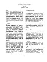
processing is used in the high Doppler bins. Figure 1 illus-
trates the concept. While not addressed in this paper, Figure 1
also suggests that varying the bandwidth as a function of tar-
get radial velocity may also be appropriate.
This paper explores signal processing techniques that
“blur” the line between SAR and GMTI processing. We fo-
cus on STAP implementations using long GMTI CPIs as well
as SAR-like processing strategies for detecting slow-moving
targets. The performance of the techniques is demonstrated
using ideal clutter covariance analysis as well as radar sam-
ple simulations and collected data. Discussion of multires-

olution processing has been previously presented [5, 6].
In this paper, we augment the analysis with SAR-derived
knowledge-aided constraints to improve performance in an
environment that includes large discrete scatterers that in-
duce elevated false-alarm rates.
Section 2 presents the details about the radar simula-
tion used to analyze the signal processing algorithms. In
Section 3, we consider the advantages of long CPIs using
ideal covariance analysis. Section 4 introduces three adaptive
2 EURASIP Journal on Applied Signal Processing
MTI mode
narrow bandwidth
short CPI
Determined by
aperture, sample
support, environment
SAR mode
wide bandwidth
long CPI
Targets outside mainbeam clutter
STAP
∗
, DPCA, conventional beam
Targets
closeorin
the mainbeam
clutter
STAP
∗
? SAR

Moving
targets
Stationary
targets
Decreasing target radial velocity
Figure 1: Illustration of multiresolution processing concept. The “∗” indicates that the targets in the training data is an issue.
signal processing techniques that attempt to exploit long
CPIs to improve the detection performance of very slow-
moving targets. Section 5 presents performance results of the
techniques using simulated and collected radar data. Finally,
Section 6 summarizes the findings and outlines areas for fur-
ther research.
2. GMTI RADAR SIMULATION
Simulated radar data was produced for use in analyzing the
signal processing techniques proposed in this paper. Under
previous simulation efforts [7–10] where the CPI length was
short, it was possible to ign ore certain effects due to platform
motion during a CPI (e.g., range walk and bearing angle
changes of the ground scattering patches). A description of
the simulation methodology has been previously presented
in [5, 6]. It is presented here also for completeness. Under
the current effort, however, where we are specifically inter-
ested in long CPIs, it was important to produce simulated
data that accurately accounts for the effects of platform mo-
tion. Therefore, the simulated data samples were computed
as
x( k, n, m)
=
P
c


p=1
α
p
t
p,m
s

kT
s
−
r
p,m
c

e
j(φ
n
(θ
p,m
)−2πr
p,m
/λ)
,(1)
where k is the range bin index, m = 1, 2, , M is the pulse
index, n
= 1, 2, , N is the channel index, N is the num-
ber of spatial channels, M is the number of pulses, s(t) is the
radar waveform (LFM chirp compressed using a 30 dB side-
lobe Chebychev taper), T

s
is the sampling interval, λ is the
radio wavelength, c is the speed of light, r
p,m
and θ
p,m
are the
two-way range and direction of arrival (DoA), respectively,
for the pth ground clutter patch on the mth pulse, α
p
is the
complex ground scattering coefficient, φ
n
(θ
p,m
) is the relative
phase shift of the nth ar ray channel for a signal from DoA
θ
p,m
, P
c
is the number of clutter scatterers in the scene, and
t
p,m
is a random complex modulation from pulse to pulse
due to internal clutter motion (ICM) [11].
Simulated
ground clutter area
(Clutter patches
∼ 6m× 6m)

Platform
heading
Nominal subarray
pattern mainbeam
Figure 2: Simulation geometry.
The ideal clutter covariance matrix for a given range sam-
ple (i.e., range bin) is given as (e.g., [12])
R
k
=
P
c

p=1


α
p


2
v
p
v
H
p
◦ T
icm
,(2)
where

◦ denotes the matrix Hadamard (elementwise) prod-
uct and v
p
is the MN × 1 space-time response (“steering”)
vector [12] of the pth scattering patch. The elements of v
p
are ordered such that the first N elements are the array spatial
snapshot for the first pulse, the next N elements are the spa-
tial snapshot for the second pulse, and so on. The elements
of v
p
are given as
ν
p

N(m − 1) + n

= s

kT
s
−
r
p,m
c

e
j(φ
n
(θ

p,m
)−2πr
p,m
/λ)
. (3)
Finally, we note that the matrix T
icm
is a covariance ma-
trix taper [13] that accounts for the decorrelation among the
pulses due to ICM (i.e., due to t
p,m
) and is based on the
Billingsley spectral correlation model for wind-blown foliage
decorrelation [14].
The simulation geometry is shown in Figure 2. The plat-
form is flying north at an altitude of 11 km and the radar
antenna is steered to look aft 17
◦
. The clutter environment
consists of an area at a slant range of 38 km that is slightly
wider in the cross-range dimension than the antenna sub-
array pattern. The area is comprised of a grid of scattering
J.S.BerginandP.M.Techau 3
Table 1: Simulation parameters.
Parameter Value (units)
Frequency X-band
Bandwidth 10 MHz
PRF 1 kHz
Number of pulses 512
Antenna 3.5m

× 0.3m
Number of subarrays 6 (50% overlap)
Subarray pattern Hamming (∼ 40 dB sidelobes)
CNR 40 dB per subarray/pulse
Platform speed 125 m/s
Azimuth steering direction 17
◦
re. broadside
Platform altitude 11 km ASL
Slant range 38 km
patches of dimension 6 m × 6 m. The complex amplitudes of
the scattering patches are i.i.d. Gaussian with zero mean and
variance that results in a clutter-to-noise ratio for a single
subarray and pulse of approximately 40 dB at the slant range
of 38 km. A list of system parameters is given in Table 1 .
We note for this particular scenario that a given scattering
patch in the mainbeam will “walk” on the order of one range
resolution cell relative to the platform (due to platform mo-
tion) during the course of the 0.5-second CPI.
3. IDEAL COVARIANCE ANALYSIS
This section presents the results of GMTI system perfor-
mance analyses as a function of CPI length using the ideal
ground clutter covariance matrix.
3.1. Ground clutter cancellation
The ideal clutter covariance was used to investigate GMTI
performance as a function of the CPI length using optimal
space-time beamforming. The goal of this analysis was to
establish an understanding of the theoretical advantages of
using longer CPIs to detect moving targets. We employed
a multi-bin post-Doppler space-time beamformer [15]with

weights computed using the ideal clutter-plus-thermal-noise
covariance matrix,
w
o

θ, f
d

=

H
H

R
k
+ R
n

H

−1
H
H
v

θ, f
d

,(4)
where H represents a matrix transformation of the space-

time data into post-Doppler channel space (i.e., each column
of H represents one of the adjacent Doppler filters), R
n
is the
covariance matrix of the thermal noise, and v(θ, f
d
) is the
space-time response of a signal with DoA θ and Doppler shift
f
d
. We note that v(θ, f
d
) is the usual space-time steering vec-
tor [12] and does not include the effects of range walk. Also,
in the SINR results, we do not account for the small losses
that this will cause due to mismatch with a true target re-
sponse.
Figure 3 shows the signal-to-interference-plus-noise ra-
tio (SINR) loss as a function of CPI length for the cases with
and without ICM. SINR loss is defined as the system sensitiv-
ity loss relative to the performance in an interference-free en-
vironment [12]. In this case, we have used 7 adjacent Doppler
bins formed via orthogonal Doppler filters. It was found that
using more Doppler bins resulted in negligible gain in perfor-
mance. It is interesting to note that the shape of the filter re-
sponse versus Doppler does not improve significantly as the
CPI length is increased suggesting that the improvements in
minimum detectable velocity (MDV) (i.e., the lowest r adial
velocities detectable by the system) will be modest for longer
CPIs.

The curves in Figure 3 do not fully characterize the gain
in system sensitivity with increasing CPI length given a con-
stant power and aperture. Figure 4 shows the SINR for the
cases shown in Figure 3, assuming that the interference-free
SNR of the target using eight pulses in a CPI is 17 dB. Thus
we see the effects on MDV of the increased sensitivity gain
achieved by using more pulses (i.e., longer integration time).
If we assume that 12 dB SINR is required for detection, then
the MDV for each CPI length occurs when that curve inter-
sects the SINR
= 12 dB level.
Figure 5 indicates the MDV value as a function of the CPI
length for the cases with and without ICM. We see that the
gain in MDV drops off rapidly as the CPI length is increased.
Therefore, we conclude that arbitrarily increasing the CPI
will not result in significant gains in MDV beyond a certain
point which will generally be determined by the system aper-
ture size and ICM (or other sources of random modulations
from pulse to pulse).
3.2. Targets in the secondary training data
While longer CPIs do not significantly improve the ability
to resolve targets from clutter beyond a certain point due
to the distributed Doppler response of ground clutter as ob-
served by a moving airborne platform, there is the potential
that longer CPIs will help better resolve targets in the scene.
This has the obvious benefits of improving tracker perfor-
mance by allowing clusters of closely spaced targets to be re-
solved.
An even greater potential benefit of the improved abil-
ity to resolve targets is that targets corrupting the secondary

training data [9, 16]willbelesslikelytoresultinlosseson
other nearby targets. This is illustrated in Figure 6 where the
SINR loss is shown for the case when a single target is in-
jected into the ideal clutter covariance with a target radial
velocity of 3.9 m/s. We see that as the CPI length is increased
the region incurring losses due to the target in the covari-
ance gets increasingly narrow indicating that it will only take
a very small relative Doppler offset between two targets to
avoid mutual cancellation. Quantifying the effectiveness of
longer CPIs in mitigating the problem of targets in the sec-
ondary training data for realistic moving target scenarios is
an area for future research.
4 EURASIP Journal on Applied Signal Processing
0
−5
−10
−15
−20
−25
−30
SINR/SNR
0
(dB)
−6 −4 −20246
Target radial velocity (m/s)
8
32
64
128
256

512
(a)
0
−5
−10
−15
−20
−25
−30
SINR/SNR
0
(dB)
−6 −4 −20 2 46
Target radial velocity (m/s)
8
32
64
128
256
512
(b)
Figure 3: Optimal SINR loss. (a) No ICM. (b) Billingsley ICM. The legend indicates the number of pulses used in a CPI.
30
20
10
0
SINR (dB)
−6 −4 −2024 6
Target radial velocity (m/s)
8

32
64
128
256
512
(a)
30
20
10
0
SINR (dB)
−6 −4 −20246
Target radial velocity (m/s)
8
32
64
128
256
512
(b)
Figure 4: Optimal SINR assuming eight-pulse SNR is 17 dB. (a) No ICM. (b) Billingsley ICM. The legend indicates the number of pulses
used in a CPI.
4. ADAPTIVE ALGORITHMS
This section details three adaptive signal processing algo-
rithms that exploit long CPIs to improve the detection per-
formance of very slow-moving targets. The goal is to eval-
uate the utility of long CPIs for performance improvements
including evaluating the hypothesis that longer CPI data may
be exploited to increase the number of samples available
for covariance estimation without significantly increasing the

range swath over which samples are drawn. It is assumed that
this will be advantageous in realistic clutter environments
where variations in the terrain and land cover often limit the
stationarity of the radar data in the range dimension to nar-
row regions.
4.1. Sub-CPI processing
The ideal covariance matrix analysis presented in Section 3.1
suggests that for a given system it may not be necessary to
coherently process all the pulses in a long CPI to approach
J.S.BerginandP.M.Techau 5
4
3
2
1
0
MDV (m/s)
0 100 200 300 400 500
Number of pusles
No ICM
ICM
Figure 5: MDV based on the curves shown in Figure 4.
0
−5
−10
−15
−20
−25
−30
SINR/SNR
0

(dB)
−6 −4 −20 2 4 6
Target radial velocity (m/s)
8
32
128
256
Figure 6: Optimal SINR loss for the case when a single target cor-
rupts the secondary training data. The target corrupting the train-
ing data has a target r adial velocity of approximately 3.9m/s. The
legend indicates the number of pulses used in a CPI.
the optimal MDV. Therefore, if many pulses are available, it
may be advantageous to limit the coherent processing inter-
val, but exploit the extra pulses to increase the training data
set for covariance estimation. It is important to note that the
potential advantage of reducing effects due to targets in the
training data will not be realized in this case since the coher-
ent processing interval is still short. For example, Figure 7 il-
lustrates an approach for segmenting the pulses to form data
snapshots that can be used for covariance matrix estimation.
In this case, the sample covariance matrix is computed as

R =
1
KK

K

k=1
K



k

=1
x
k,k

x
H
k,k

,(5)
X
K,1
X
K,2
··· X
K,k

··· X
K,K

X
k,1
X
k,2
··· X
k,k


··· X
k,K

X
1,1
X
1,2
··· X
1,k

··· X
1,K

Pulse
Range
···
···
···
···
Element
···
···
···
Figure 7: Illustration of sub-CPI segmentation.
where x
k,k

is the snapshot from the kth range bin and k

th

sub-CPI. We note that vector x
k,k

is formed by reordering the
matrix X
k,k

as shown in Figure 7 so that the first N elements
are the spatial samples on the first pulse, the next N elements
are the spatial samples on the second pulse, and so on. The
quantity K is the number of training range samples and K

is the number of sub-CPIs used in the training. The effect of
varying these quantities is demonstrated in Section 5.
The covariance estimate based on the sub-CPI data is
used to compute an adaptive weight vector that can gener-
ally be applied to each of the sub-CPIs in the range bin under
test to form K

complex beamformer outputs. Methods for
combining these outputs either coherently or incoherently
to improve the system sensitivity are an area for future re-
search. It is worth noting, however, that in general it should
be possible to coherently combine the outputs if unity gain
constraints are employed in the beamformer calculation and
delays in the target response in each sub-CPI relative to the
start of the CPI are accounted for.
While this approach is interesting from a theoretical
point of view in that it shows an alternative approach for
exploiting a long CPI to increase training samples without

increasing the training window, it was found to be difficult
to implement in practice. This is due to the fact that when
used to achieve highly localized training, this technique ex-
acerbates the problem of target self-nulling due to the range
sidelobe contamination of the training data. Also, we would
not expect the sub-CPI training approach to help mitigate
the problem of targets in the training data since the coherent
processing will still occur over a short CPI.
4.2. Long-CPI post-Doppler
An alternative approach to sub-CPI processing is to Doppler
process (e.g., discrete Fourier transform) the CPI using all
the pulses and then apply adaptive techniques similar to
multi-bin post-Doppler STAP [15]. In the case when the CPI
is very long, it may be advantageous to employ SAR process-
ing (instead of Doppler processing) that accounts for range
walk of the scatterers in the scene that results from platform
motion. This approach has been proposed previously [17].
Figure 8 illustrates the concept. We note that this technique
will take advantage of the property of long CPIs to reduce
6 EURASIP Journal on Applied Signal Processing
Cell under test
Training cells
Antenna #1
Antenna #2
Antenna #3
Antenna #N
.
.
.
.

.
.
x(N
× 1)
Cross-range
Range
Figure 8: Illustration of long-CPI post-Doppler processing. Note
training is possible in both range and cross-range.
Physical aperture
mainbeam
Clutter spatial
responses in
these Doppler
bins will be
approximately
linearly
dependent
.
.
.
Angle
Doppler
Figure 9: Illustration of clutter ridge and large difference in angular
and temporal resolution for long CPIs.
the effects of targets in the secondary training data as long as
multiple adaptive Doppler bins are employed.
In the simplest form, the data from each antenna is used
to form a spatial-only covariance matr ix estimate using data
from Doppler and range bins (or cross-range and range pix-
els in the case of SAR preprocessing). If we only employ

data from adjacent range bins for training, this technique
(in the case of Doppler processing) is identical to factored
time-space beamforming [12] (i.e., single-bin post-Doppler
adaptive processing). In [17] it was proposed that adjacent
cross-range (or Doppler bins) should also be included in the
training set. This may at first seem unusual in the context
of GMTI STAP for which training using only adjacent range
bins is the common practice.
Figure 9 illustrates why it is efficacious to use data from
adjacent Doppler bins to estimate the correlation among the
spatial channels when the CPI is long.
We see that since the Doppler resolution is much
finer than the spatial resolution, clutter patches in adjacent
Doppler bins will have highly linearly dependent spatial re-
sponses and therefore can be averaged to improve the spatial
covariance matrix estimate [5, 6]. The azimuth beamwidth
0
−5
−10
−15
−20
−25
−30
SINR/SNR
0
(dB)
−6 −4 −20 2 4 6
Target radial velocity (m/s)
1
11

21
41
Figure 10: Effect of Doppler training region size in long-CPI post-
Doppler processing. The training bins are centered around and
include the bin under test. The legend indicates the number of
Doppler training bins used.
of the physical aperture is given as
δ
a
=
λ
L
,(6)
where L is the length of the aperture in the horizontal di-
mension. The azimuth beamwidth of the synthetic aperture
(azimuthal extent of the ground clutter in a single Doppler
bin) is given as [18]
δ
d
=
λ
2L
eff
=
λf
P
2ν
p
M
,(7)

where L
eff
is the distance traveled by the platform during the
CPI, f
p
is the PRF, and ν
p
is the platform speed. The ratio of
δ
a
to δ
d
,
f
res
=
δ
a
δ
d
=
2ν
p
M
Lf
p
,(8)
gives an approximate expression for the number of Doppler
bins w ithin the mainbeam and thus the number of adjacent
Doppler bins that can be used as training samples. For the

system simulation discussed in Section 2, the quantity f
res
=
36.6.
Figure 10 demonstrates the effects of increasing the num-
ber of adjacent Doppler bins used in the training set for
the single adaptive bin case (i.e., factored time-space adap-
tive beamforming). The total number of pulses in the CPI
is 256 which results in f
res
= 18.2 and we note that a
65 dB sidelobe level Chebychev taper is applied across the
256 pulses prior to Doppler processing. In this example, the
ideal spatial-only covariance matrix for each of the adjacent
Doppler bins used in the training strategy was computed and
then summed together to form the “ideal” (ensemble average
of the) estimated covariance matrix. T his covariance matrix,
J.S.BerginandP.M.Techau 7
which takes into account the effects of training over adjacent
Doppler bins, was then used to compute SINR loss. As ex-
pected, when the number of bins exceeds f
res
= 18.2, the
SINR loss begins to degrade.
More sophisticated versions of the long-CPI post-
Doppler algorithm will include multiple temporal degrees
of freedom. In [17] multiple adjacent SAR pixels were com-
bined adaptively along with the spatial channels to form the
adaptive clutter filter. When training samples are only cho-
sen from adjacent range bins, this version of the algorithm is

similar to multi-bin post-Doppler element-space STAP [15].
In fact, if the preprocessing uses Doppler filters instead of
SAR processing, the algorithm is mathematically equivalent
to multi-bin post-Doppler STAP.
Choosing training samples from adjacent Doppler and
range bins is not as straightforward as it was in the sin-
gle a daptive bin case since the samples can be chosen to be
either overlapped or nonoverlapped in Doppler. In [17]it
was observed that the multipixel covariance estimation pro-
cess introduced “artificial” increases in the correlation of the
background thermal noise between pixels when the over-
lapped training samples were used since the thermal noise
for two overlapping training samples will typically be corre-
lated. Theoretical analysis of estimators that use overlapping
training data to estimate the multipixel correlation matrix is
an area for future research.
4.3. SAR-derived knowledge-aided constraints
In [19–22] the application of knowledge-aided constraints
was developed. In that analysis, the ground clutter is as-
sumed to be known to some degree and the interference co-
variance matrix is assumed to be the sum of three compo-
nents: a known clutter covariance component, an unknown
clutter covariance component, and thermal noise, typically
uncorrelated among the channels and pulses. This struc-
ture is used to derive a post-Doppler channel-space weight
that incorporates the known clutter covariance component
as a quadratic constraint. The approach to finding the op-
timal weight vector for the mth channel w
m
is to solve the

following constrained minimization:
min
w
m
E



w
m
x
m


2

such that
⎧
⎪
⎪
⎪
⎪
⎨
⎪
⎪
⎪
⎪
⎩
w
m

v
m
= 1,
w
H
m
R
c,m
w
m
≤ δ
d,m
,
w
H
m
w
m
≤ δ
l,m
,
(9)
where for a desired reduced-DoF orthonormal MN
× D (D<
MN) transformation H
m
,wehave
x
m
= H

H
m
x, v
m
= H
H
m
v,
R
c,m
= H
H
m
R
c
H
m
, R
m
= H
H
m

R
xx
H
m
,
(10)
and where R

c
represents the known component of the inter-
ference (e.g., (2)),

R
xx
is the usual sample estimate of the co-
variance matrix, and δ
d,m
and δ
L,m
are arbitrarily small con-
stants.
In (9), the first constraint is the usual point con-
straint [12] while the third constraint introduces diagonal
loading to the solution. The second constraint incorporates
a priori knowledge into the solution by forcing the space-
time weights to tend to be orthogonal to the known clutter
subspace. The result, derived in [21, 22], is
w
m
=

R
m
+ β
d,m
R
c,m
+ β

L,m
I
D

−1
v
m
v
H
m

R
m
+ β
d,m
R
c,m
+ β
L,m
I
D

−1
v
m
=

R
m
+ Q

m

−1
v
m
v
H
m

R
m
+ Q
m

−1
v
m
,
(11)
where Q
m
= β
d,m
R
c,m
+ β
L,m
I
D
, I

D
is a D × D identity matrix,
and β
d,m
and β
L,m
are the colored and diagonal loading lev-
els, respectively, that may be specific to each transformation.
Note that β
d,m
and β
L,m
are related to the constraint values
δ
d,m
and δ
L,m
via two coupled nonlinear inequality relations
[22].
It is interesting to note that the solution given in (11)
results in a “blending” of the information contained in the
sample covariance matrix and the a priori clutter model.
Therefore, the solution has the desirable property of combin-
ing adaptive and deterministic filtering. In fact, the solution
will provide beampatterns that are a mix between the fully
adaptive pattern, a fully deterministic filter, and the conven-
tional pattern represented by the constraint v
m
. An interest-
ing area for future research will be to develop rules for setting

the covariance “blending” factors based on the characteris-
tics of the operating environment (e.g., expected density of
targets, terrain type, etc.) derived from auxiliary databases.
Additional discussion regarding the selection of the loading
levels may be found in [19].
We note that the beamformer weights in (11)canbe
re-written to permit inter pretation as a two-stage filter
where the first stage “whitens” the data vector using the
a priori covariance model and then is followed by an adaptive
beamformer based on the whitened data [19]. This leads us
to consider the possibility of using SAR data to identify dis-
crete scatterers, generate a space-time response for that dis-
crete scatterer using the observed spatial response and a pre-
dicted temporal response, and using that response to build a
prefilter/colored-loading matrix to minimize the false-alarm
impact of the discrete scatterers in a given scenario. This pro-
cess is illustrated in Figure 11 and described in more detail in
[22].
5. RESULTS
The simulated data discussed in Section 2 along with exper-
imentally collected data was used to test the adaptive pro-
cessing techniques described in Section 4. Five range samples
were simulated and an ideal covariance matrix for the center
range bin was generated. Adaptive weights were estimated
from the data samples using the various training strategies
and then (for the simulated data) applied to the ideal covari-
ance matrix to compute the SINR loss metric.
8 EURASIP Journal on Applied Signal Processing
24.5
24

23.5
23
22.5
22
21.5
(km)
−10 −50510
Doppler (m/s)
60
50
40
30
Power (dB)
Time: 21 s
(a)
Discrete
s(θ
p
)
Ant. #1
Ant. #2
Ant. #3
Cross-range
Range
v(θ
p
,f
p
) = (H
H

m
t( f
p
)

s(θ
p
))
t
[m]
( f
p
) = exp( j2πmf
p
T
pri
)
(b)
R
c,m
=
P
c

p=1
v
m
(θ
p
,f

p
)v
H
m
(θ
p
,f
p
)
w
m
= γ(R
m
+ β
d,m
R
c,m
+ β
L,m
I)
−1
v
m
(c)
Figure 11: SAR-derived colored-loading processing algorithm. (a) Step 1: threshold “low-resolution” SAR map to detect discrete clutter.
(b) Step 2: form space-time response for each discrete and transform to post-Doppler space (use observed spatial response). (c) Step 3: use
response to form a range-dependent “loading” matrix for each Doppler bin, add to sample covariance, and run STAP processor.
5.1. Sub-CPI processing
Figure 12 shows the SINR loss for sub-CPI processing as a
function of the number of pulses in the sub-CPI for three

cases: (1) range-only training, (2) sub-CPI only training,
and (3) range and sub-CPI training. The adaptive algorithm
was multi-bin post-Doppler channel-space STAP employing
three adjacent adaptive Doppler bins. Diagonal loading with
a level of 0 dB relative to the thermal noise was used in all
cases.
We see that range-only training results in poor perfor-
mance since there are too few training samples to support the
adaptive DoFs. Performance is improved by using the sub-
CPIs from a single range bin as the training data. In this case,
the number of training samples is equal to the total number
of pulses (512) divided by the number of pulses in the sub-
CPI. Thus, for the examples shown, the number of sub-CPI
training samples is 64, 32, and 16 for the 8, 16, and 32 pulse
sub-CPI cases, respectively.
Finally, we see that if training samples are chosen from
both sub-CPIs and range bins, we get near-optimal (relative
to the ideal covariance case) performance. In this case, the
total number of training samples is the number of range bins
multiplied by the number of sub-CPI segments. Thus the
number of samples for the cases shown is 320, 160, and 80 for
the 8, 16, and 32 pulse sub-CPI cases, respectively. This ex-
ample demonstrates that highly localized training regions in
range may be possible if training data is augmented with sub-
CPI data snapshots. This strategy will generally be the most
advantageous in nonhomogeneous clutter environments.
5.2. Long-CPI post-Doppler
Figure 13 shows the SINR loss results for the long-CPI post-
Doppler processing technique. The results are presented for
three cases: (1) a single adaptive Doppler bin, (2) three

adjacent adaptive Doppler bins with overlapped Doppler
training snapshots, and (3) three adjacent adaptive Doppler
bins with nonoverlapped Doppler training snapshots. In each
case, the CPI length is 512 and training data from 21 ad-
jacent Doppler filters is used in the covariance estimation.
In this case, f
res
= 36.6, but a value of 21 was used to en-
sure that no losses were incurred due to overextending the
Doppler training window. We also note that the single adap-
tive Doppler bin case employs a 65 dB sidelobe level Cheby-
chev taper across the 512 pulses prior to Doppler processing.
Figure 13(a) (“1 adaptive bin”) has a black dashed curve
which represents the case when five range samples are used
to estimate the spatial covariance matr ix which in this case
has dimension six due to the six spatial channels employed
in the simulation. We note that diagonal loading at a level of
0 dB relative to the thermal noise floor was required so the
estimated covariance matrix could be inverted. We see that
the range-only training results in poor performance due to
the small number of training samples.
We see, however, that when adjacent Doppler bins are
used for training, we get much better performance (dot-
ted and dash-dotted curves). The dotted curve uses adjacent
Doppler bins and five range samples for training data and the
dash-dotted curve uses adjacent Doppler bins from a single
range bin. We see that the best performance is achieved when
multiple adaptive Doppler bins are employed and train-
ing is performed using both adjacent range bins and over-
lapping Doppler samples. The generally poor performance

when only adjacent Doppler samples are used is most likely
attributed to the correlation of the thermal noise among the
training samples which results in a poor estimate of the back-
ground ther mal noise statistics. Developing a better under-
standing of this phenomenon via analysis and simulation is
an area for future research.
The data set was generated both with and without targets
so clutter-only training data is available for use in analyzing
J.S.BerginandP.M.Techau 9
0
−5
−10
−15
−20
−25
−30
SINR/SNR
0
(dB)
−6 −4 −202 46
Target radial velocity (m/s)
8
16
32
(a)
0
−5
−10
−15
−20

−25
−30
SINR/SNR
0
(dB)
−6 −4 −202 46
Target radial velocity (m/s)
8
16
32
(b)
0
−5
−10
−15
−20
−25
−30
SINR/SNR
0
(dB)
−6 −4 −20 2 4 6
Target radial velocity (m/s)
8
16
32
(c)
Figure 12: SINR loss for sub-CPI t raining. (a) Range-only training (five range bins). (b) Training using sub-CPIs from a single range bin.
(c) Training using sub-CPIs from five range bins. The black dashed line is the optimal full-DoF STAP performance. The legend indicates the
number of pulses u sed in a CPI.

algorithms. For example, the clutter-only training data can
be used to compute adaptive weights and can then be ap-
plied to the clutter-plus-targets data. This allows us to iso-
late the effects of targets corrupting the secondary training
data. Figure 14 shows the beamformer output for three-bin
post-Doppler STAP with 48 training samples chosen in the
range dimension only. Also shown is an overlay of ground
truth targets. The result is shown for a 64-pulse CPI and a
256-pulse CPI. We see that when clutter-only training data
is used for training, both the 64-pulse and 256-pulse CPIs
detect the same targets including the very slow movers near
the clutter ridge (0 m/s Doppler). When the clutter-plus-
targets training data is used, however, the 256-pulse CPI de-
tects significantly more targets for the reasons discussed in
Section 3.2. We note that more than 256 pulses (0.25-second
CPI) were not used to avoid significant losses due to range
and Doppler walk. In cases when longer CPIs than shown
here are employed, more sophisticated preprocessing steps
than simple Doppler processing will be required (e.g., SAR
image formation).
Figure 15 summarizes the number of detections as a
function of threshold level (relative to thermal noise) for
three values of the CPI length. We note that the threshold
values shown are for the 64-pulse case and that the thresh-
old values for the 128- and 256-pulse cases were increased
by 3 dB and 6 dB, respectively, to account for the increased
integration gain. Threshold crossings were declared detec-
tions if they were within a single range and Doppler bin of
a target in the ground truth. We see that when clutter-only
data is used for tra ining, each CPI length produces approxi-

mately the same number of detections. When the targets are
included in the training, however, the longer CPI results in
a significant increase in detections. We note that there are a
total of 38 targets in the scenario.
10 EURASIP Journal on Applied Signal Processing
0
−5
−10
−15
−20
−25
−30
SINR/SNR
0
(dB)
−6 −4 −20 2 4 6
Target radial velocity (m/s)
Ideal
5ranges
1range
(a)
0
−5
−10
−15
−20
−25
−30
SINR/SNR
0

(dB)
−6 −4 −20 2 4 6
Target radial velocity (m/s)
Ideal
5ranges
1range
(b)
0
−5
−10
−15
−20
−25
−30
SINR/SNR
0
(dB)
−6 −4 −20 2 4 6
Target radial velocity (m/s)
Ideal
5ranges
1range
(c)
Figure 13: Long-CPI post-Doppler processing. (a) One adaptive bin (factored post-Doppler). The black dashed line indicates range-only
training. (b) Three adaptive bins (multi-bin post-Doppler) with overlapped training. (c) Three adaptive bins with nonoverlapped training.
legend indicates either ideal covariance matrix result or number of ranges used in training.
Figure 16 shows the beamformer output for the case
when training data from adjacent Doppler bins is employed.
In this case, a single three-bin sample was chosen on each side
of the bin under test in the Doppler dimension (we are still

using three-bin post-Doppler STAP) separated by three bins
from the bin under test over a range swath of 24 samples.
Thus the extra training samples chosen in the Doppler di-
mension are nonoverlapping and the total number of train-
ing samples is 48. We see that even in the clutter-only train-
ing case that the response of the very slow-moving targets
near 0 m/s Doppler are somewhat weaker than in the range-
only training case (Figure 14(a), 256 pulse case) indicating
that this method of training tends to reduce the ability to re-
solve slowly moving targets f rom clutter.
In the clutter-plus-targets training case, we see that in
some cases this method of training improves performance
(compare to Figure 14(b), 256 pulse case). For example, since
this method does not use training samples from the same
Doppler bin versus range, the two targets at approximately
45.25 km range that are closely spaced in Doppler are de-
tected whereas in Figure 14(b) they are not. However, there
are several targets detected in Figure 14(b) that are not de-
tected in Figure 16(b). Even though the targets corrupting
the training data are in a different Doppler bin (since the
training samples a re chosen from adjacent Doppler bins),
across the three chosen bins their response is very similar to
the 3-bin response of the target of interest. Thus they can still
contribute to nulling a target of interest.
An interesting difference between the range-only train-
ing and adjacent Doppler training results is a noticeable re-
duction in the amount of undernulled clutter, particularly
around the clutter ridge. This indicates that the more local-
ized training (the training range swath here is 360 m as op-
posed to 720 m in Figure 14) as well as the inclusion of the

J.S.BerginandP.M.Techau 11
46.5
46
45.5
45
44.5
Range (km)
−6 −4 −20 2
Target radial velocity (m/s)
18
16
14
12
10
8
6
Power (dB)
(a)
46.5
46
45.5
45
44.5
Range (km)
−6 −4 −20 2
Target radial velocity (m/s)
18
16
14
12

10
8
6
Power (dB)
(b)
46.5
46
45.5
45
44.5
Range (km)
−6 −4 −20 2
Target radial velocity (m/s)
18
16
14
12
10
8
6
Power (dB)
(c)
46.5
46
45.5
45
44.5
Range (km)
−6 −4 −20 2
Target radial velocity (m/s)

18
16
14
12
10
8
6
Power (dB)
(d)
Figure 14: Beamformer output for range-only training. (a) and (c) represent clutter-only training data for 64 and 256 pulses, respectively.
(b) and (d) represent clutter-plus-targets training data for 64 and 256 pulses, respectively. Magenta circles are ground truth. Mainbeam
clutter at 0 m/s.
range bin of interest in the training set results in improved
clutter cancellation performance which is the expected re-
sult.
5.3. SAR-derived knowledge-aided constraints
The Tuxedo radar is a data collection platform with an X-
band system with a three-phase center antenna array. The
system collects very long CPIs (greater than ten seconds) that
can be used to form multiaperture synthetic aperture radar
images. For the examples shown in this paper, only a subset
of the pulses spanning a more t ypical GMTI CPI (less than
0.5second)wasused.ThedatasetwascollectedatCamp
Navajo, Ariz, in a desert environment exhibiting very little
terrain relief.
The scenario does include significant strong clutter dis-
cretes scatterers, however, due to various man-made struc-
tures (buildings, towers, etc.). For example, Figure 17(a)
shows the range-Doppler map for the beamformer output
for a single azimuth steering direction. We clearly see the

mainbeam clutter which generally consists of benign under-
lying ground clutter plus large discretes in various range bins.
This type of environment can cause problems for STAP since
omitting the range bin under test from the covariance ma-
trix estimate can lead to severe undernulled clutter. This sit-
uation can be addressed using the technique described in
Section 4.3.
A long GMTI CPI (or “low-resolution SAR”) image was
formed such as the one in Figure 17(a) and thresholded to
extract the largest discretes. Figure 17(b) shows the 254 dis-
cretes extracted from the Tuxedo data by applying a 70 dB
threshold to the image in Figure 17(a). We note that this gen-
eral approach has been previously proposed [23], however,
this implementation varies significantly in that it uses the
colored-loading framework and includes an automatic cal-
ibration scheme. We also note that target cancellation will in
general be avoided since the target-to-clutter ratio is expected
to be low for the chosen long CPI range-Doppler processing
output.
12 EURASIP Journal on Applied Signal Processing
35
30
25
20
15
10
5
Number of detections
8101214161820
Threshold (dB)

M
= 64
M
= 128
M
= 256
Figure 15: Number of detections. The threshold values shown are for the 64-pulse case. The solid lines represent the clutter-plus-targets
training and the dashed lines represent the clutter-only training.
46.5
46
45.5
45
44.5
Range (km)
−6 −4 −20 2
Target radial velocity (m/s)
18
16
14
12
10
8
6
Power (dB)
(a)
46.5
46
45.5
45
44.5

Range (km)
−6 −4 −20 2
Target radial velocity (m/s)
18
16
14
12
10
8
6
Power (dB)
(b)
Figure 16: Post-Doppler STAP with training over adjacent Doppler bins. (a) Clutter-only training for 256 pulses. (b) Clutter-plus-targets
training for 256 pulses. Magenta circles are ground truth.
Figure 18 compares the beamformer output for conven-
tional and KA-STAP using the data-derived colored-loading
matrices discussed above. The information used in the load-
ing mat rices was derived from a 0.4-second CPI and applied
to a 0.1-second CPI. This result is an example of multitem-
poral resolution processing. Both the STAP and KA-STAP re-
sults use a multi-bin post-Doppler element-space algorithm
with three bins and three channels (nine DoFs). The num-
ber of training samples was 200 with the bin under test and
three guard bins on each side of the bin under test excluded
from the training set. In both cases, there is diagonal loading
that is approximately equal to the thermal noise level and for
the KA-STAP case the maximum eigenvalue of the colored-
loading matrix of the Doppler domain colored-loading ma-
trix is approximately 30 dB above the thermal noise level.
Finally, we note that the computed beamforming weights in

all cases have been normalized to give unit gain on white
noise.
We see that many of the “streaks” in the conventional
STAP result (see arrow markers on the plot) caused by
undernulling of the strong discretes have been eliminated in
the KA-STAP result. The conclusion is that by including data-
derived knowledge of the discrete locations and their spatial
responses in the KA-STAP approach will lead to significantly
fewer false alarms and/or improved detection sensitivity than
conventional STAP.
Thirty-five GMTI CPIs were generated from the 40 000
pulses of coherent Tuxedo data by taking a block of pulses
every second. GMTI CPIs consisting of 128 pulses (approx-
imately 100 milliseconds) and 32 pulses (approximately 25
J.S.BerginandP.M.Techau 13
0.3
0.2
0.1
0
−0.1
−0.2
Range re. aim point (km)
−50 5
Doppler (m/s)
5 10152025
Power (dB)
(a)
0.3
0.2
0.1

0
−0.1
−0.2
Range re. aim point (km)
−505
Doppler (m/s)
5 10152025
Power (dB)
(b)
Figure 17: A portion of the Tuxedo beamformed range-Doppler
clutter map (“low-resolution SAR”) for Camp Navajo, Ariz. (a)
Low-resolution SAR map with an overlay of “detected” clutter dis-
cretes (dark grey dots) used to form the colored-loading matrix. (b)
STAP beamformer output with same overlay of discretes. CPI length
is 0.4 second. The markers are the locations of GPS-instrumented
ground targets.
milliseconds) were considered. The radial velocities of two
of the targets, a five-ton truck and an HMMWV, are plot-
ted over time in Figure 19.Wenotethatat15secondsand
approximately 32 seconds, the two target radial velocities co-
incide (i.e., both are in the same Doppler bin).
0.3
0.2
0.1
0
−0.1
−0.2
Range re. aim point (km)
−50 5
Doppler (m/s)

2 4 6 8 10 12 14
Power (dB)
(a)
0.3
0.2
0.1
0
−0.1
−0.2
Range re. aim point (km)
−50 5
Doppler (m/s)
2 4 6 8 10 12 14
Power (dB)
(b)
Figure 18: Comparison of beamformer output for Tuxedo data.
(a) Traditional STAP. (b) STAP with colored loading. Arrows mark
some of the clutter discretes that lead to undernulled clutter in the
traditional STAP case.
Now consider, for a 25-millisecond CPI using the algo-
rithm of Figure 11, the target beamformer output power as
a function of time (CPI). Two training window sizes were
used, 200 m and 60 m. The larger window size results in one
of the targets being included in the training set of the other
14 EURASIP Journal on Applied Signal Processing
2
0
−2
−4
−6

Doppler (m/s)
0 5 10 15 20 25 30 35
Time (s)
HMMWV
5-ton truck
Figure 19: Target radial velocity as a function of time.
50
40
30
20
10
0
Power (dB)
0 5 10 15 20 25 30 35
Time (s)
HMMWV
HMMWV, loc
5-ton
5-ton, loc
Figure 20: Beamformed target power using knowledge-aided STAP
and a 25-millisecond CPI. The shorter training window (60 m) is
indicated by “loc.”
50
40
30
20
10
0
Power (dB)
0 5 10 15 20 25 30 35

Time (s)
HMMWV
HMMWV, loc
5-ton
5-ton, loc
Figure 21: Beamformed target power using knowledge-aided STAP
and a 100-millisecond CPI. The shorter training window (60 m) is
indicated by “loc.”
and vice versa (e.g., the HMMWV is included in the training
for the range bin corresponding to the five-ton truck) while
this does not result with the smaller training window. The
beamformed target output power is shown in Figure 20 as
a function of time. We see that when the two target radial
velocities coincide, there is a significant reduction in the tar-
get power out of the beamformer for the HMMWV when
using the larger training window. The shorter training win-
dow does not result in the same effect. We note that the same
does not happen with the five-ton truck. This is most likely
due to the lower power of the HMMWV.
A 100-millisecond CPI was also analyzed. The results are
shown in Figure 21. Similar effects are observed at time 32
seconds as were observed in Figure 20.However,attime15
seconds the same reduction in beamformed target power
does not result for the larger training window. This is most
likely due to the spreading across multiple Doppler bins that
occurs with the five-ton truck. This spreading results from
the radial acceleration that is observed for that vehicle in
Figure 19.
6. SUMMARY
The concept of using long CPIs to improve the detection of

very slow-moving targets was investigated. The concept was
motivated by observing that airborne radars use short CPIs
to detect fast-moving targets (e.g., GMTI STAP) and very
long CPIs to detect stationary targets (e.g., SAR) so that it is
logical to assume that it may be advantageous to use longer
and longer CPIs as the assumed Doppler velocity of targets
of interest is decreased.
Theoretical analysis of optimal beamforming techniques
that cancel clutter (e.g., STAP) was used to demonstrate that
for a given system and operating environment, there is a CPI
length beyond which significant improvements in MDV di-
minish. Beyond the cutoff, the width of the antenna and phe-
nomenology such as ICM limit the MDV performance. It was
postulated, however, that the problem of targets corrupting
the training data may be significantly reduced since when the
CPI is long, it w ill require only a very small relative difference
in Doppler velocity between targets to cause enough decor-
relation so that when they corrupt the training data, the re-
sulting sensitivity losses are negligible.
While the improvements of optimal beamformers in de-
tecting very slow-moving targets tend to diminish beyond
a certain CPI length, adaptive implementations of the opti-
mal beamformers may benefit significantly from longer CPIs.
Two adaptive techniques were presented that take advantage
of the longer CPI to improve the convergence properties of
the beamformer solution and thus increase the performance
of the beamformer. It was shown that these techniques can
reduce the number of adjacent range samples required for
training which will generally improve performance in realis-
tic clutter environments where the stationarity of the ground

clutter is often limited to narrow range reg i ons due to signif-
icant terrain relief and land cover variations.
Finally, the use of ownship SAR to identify discrete scat-
terers that can increase the false-alarm rate was explored via
a colored-loading framework. The method uses the observed
response of strong scatterers to filter out these discrete scat-
terers prior to adaptive processing. Future work will attempt
to quantify the improvement in false-alarm rate and sensitiv-
ity.
J.S.BerginandP.M.Techau 15
The proposed algorithms were tested using a homoge-
neous clutter simulation that represents a nominal X-band
GMTIradarsystemaswellasexperimentaldata.Futurework
is required to determine the performance of the proposed
techniques under other conditions and for varying system
parameters such as larger scanning angles and higher band-
widths. The goal of the future work will be to develop a better
theoretical understanding of the techniques via analysis and
simulation and to determine under what operating condi-
tions and for what types of systems they are best suited.
Finally, other approaches to multiresolution processing
may prove fruitful. The concept of optimizing the radar re-
sources (i.e., CPI length and bandwidth) to improve detec-
tion performance as a function of assumed target Doppler
shift is an area that may lead to radar systems with signifi-
cantly improved ability to track ground targets.
ACKNOWLEDGMENTS
The authors would like to acknowledge Dr. Paul Monticci-
olo and MIT Lincoln Laboratory for providing the Tuxedo
data and Matlab programs that facilitated its analysis. The

authors would like also to acknowledge Dr. Joseph Guerci
of the DARPA Special Projects Office for discussions and in-
sight regarding the development of the techniques described
herein. This work was sponsored under Air Force Contract
F30602-02-C-0005.
REFERENCES
[1] />[2] KASSPER ’02: APremierEvent, Knowledge-Aided Sensor Sig-
nal Processing and Expert Reasoning Workshop Proceedings,
Washington, DC, USA, April 2002.
[3] Knowledge-Aided Sensor Signal Processing and Expert Rea-
soning Workshop Conference Proceedings, Las Vegas, Nev,
USA, April 2003.
[4] 3rd Annual (KASSPER ’04) Workshop Conference Proceed-
ings, Clearwater, Fla, USA, April 2004.
[5] J. S. Bergin, C. M. Teixeira, and P. M. Techau, “Multi-
resolution signal processing techniques for airborne radar,” in
Proceedings of the 2003 KASSPER Workshop,LasVegas,NV,
USA, April 2003.
[6] J. S. Bergin, C. M. Teixeira, and P. M. Techau, “Multi-
resolution signal processing techniques for airborne radar,”
in Proc. 2004 IEEE Radar Conference, Philadelphia, Pa, USA,
April 2004.
[7] J. S. Bergin and P. M. Techau, “High fidelity site-specific radar
simulation: KASSPER ’02 workshop datacube,” Tech. Rep. ISL-
SCRD-TR-02-105, Information Systems Laboratories (ISL),
Vienna, Va, USA, May 2002.
[8] J. S. Bergin and P. M. Techau, “High-fidelity site-specific radar
simulation: KASSPER data set 2,” Tech. Rep. ISL-SCRD-TR-
02-106, Information Systems Laboratories (ISL), Vienna, Va,
USA, October 2002.

[9] J. S. Bergin, P. M. Techau, W. L. Melvin, and J. R. Guerci,
“GMTI STAP in target-rich environments: site-specific anal-
ysis,” in Proc. 2002 IEEE Radar Conference, pp. 391–396, Long
Beach, Calif, USA, April 2002.
[10] P. M. Techau, J. R. Guerci, T. H. Slocumb, and L. J. Griffiths,
“Performance bounds for hot and cold clutter mitigation,”
IEEE Transactions on Aerospace and Electronic Systems, vol. 35,
no. 4, pp. 1253–1265, 1999.
[11] J. B. Billingsley, “Exponential decay in windblown radar
ground clutter Doppler spect ra: multifrequency measure-
ments and model,” Tech. Rep. 997, MIT Lincoln Laboratory,
Lexington, Mass, USA, July 1996.
[12] J. Ward, “Space-time adaptive processing for airborne radar,”
Tech. Rep. 1015, MIT Lincoln Laborator y, Lexington, Mass,
USA, December 1994.
[13] J.R.Guerci,“Theoryandapplicationofcovariancematrixta-
pers for robust adaptive beamforming,” IEEE Transactions on
Signal Processing, vol. 47, no. 4, pp. 997–985, 1999.
[14] P. M. Techau, J. S. Bergin, and J. R. Guerci, “Effects of internal
clutter motion on STAP in a heterogeneous environment,” in
Proceedings of 2001 IEEE Radar Conference, pp. 204–209, At-
lanta, Ga, USA, May 2001.
[15] R. C. DiPietro, “Extended factored space-time processing for
airborne radar systems,” in Proceedings of 26th Annual Asilo-
mar Conference on Signals, Systems, and Computing, vol. 1, pp.
425–430, Pacific Grove, Calif, USA, October 1992.
[16] W. L. Melvin and J. R. Guerci, “Adaptive detection in dense
target environments,” in Proceedings of 2001 IEEE Radar Con-
ference, pp. 187–192, Atlanta, Ga, USA, May 2001.
[17] A. Yegulalp, “FOPEN GMTI using multi-channel adaptive

SAR,” in Proceedings of 10th Annual Adaptive Sensor Array Pro-
cessing Workshop, MIT Lincoln Laboratory, Lexington, Mass,
USA, March 2002.
[18] M. I. Skolnik, Radar Handbook, McGraw-Hill, Boston, Mass,
USA, 1990.
[19] J. S. Bergin, C. M. Teixeira, P. M. Techau, and J. R.
Guerci, “Space-time beamforming with knowledge-aided con-
straints,” in Proceedings of Adaptive Sensor Array Processing
Workshop, MIT Lincoln Laboratory, Lexington, Mass, USA,
March 2003.
[20] C. M. Teixeira, J. S. Bergin, and P. M. Techau, “Reduced
degree-of-freedom STAP with knowledge-aided data pre-
whitening,” in Proceedings of 2003 KASSPER Workshop,LasVe-
gas, Nev, USA, April 2003.
[21] J. S. Bergin, C. M. Teixeira, P. M. Techau, and J. R. Guerci, “Re-
duced degree-of-freedom STAP with knowledge-aided data
pre-whitening,” in Proceedings of 2004 IEEE Radar Conference,
Philadelphia, Pa, USA, April 2004.
[22] J. S. Bergin, C. M. Teixeira, P. M. Techau, and J. R. Guerci,
“STAP with knowledge-aided pre-whitening,” in Proceedings
of the 2004 Tri-Service Radar Symposium, pp. 289–294, Albu-
querque, NM, USA, June 2004.
[23] W. L. Melvin, G. A. Showman, and D. J. Zywicki, “KA-
STAP Development: GTRI Update,” in Briefing Presented at
the KASSPER 2002 Program Rev iew, MIT Lincoln Laboratory,
Lexington, Mass, USA, September 2002.
Jameson S. Bergin received his B.S.E.E. and
M.S.E.E. degrees from the University of
New Hampshire. He is a Principal Engi-
neer with Information Systems Laborato-

ries, Inc., in Vienna, Virginia. He has been
with ISL since 1996. He has a background
in digital signal processing, adaptive array
processing, time series a nalysis, and com-
munications systems. At ISL, he is mod-
eling terrain-specific radar phenomenology
including propagation, clutter, and hot clutter (terrain-scattered
interference) and analyzing system performance. He has developed
16 EURASIP Journal on Applied Signal Processing
simulation and analysis tools for STAP algorithm development and
applied these tools to the analysis of both simulated and experi-
mental data. At the University of New Hampshire, he was a Member
of the Meteor Wind Radar Laboratory where his research included
the use of higher-order spectral analysis techniques to detect non-
linear mixing of wind components in the upper atmosphere. In ad-
dition, he has analyzed problems such as radar system degradation
due to Doppler quantization and nonuniform sampling.
Paul M. T echau received his M.S.E. de-
gree from the University of Michigan and
his B.S.E.E. degree from the University of
Akron. He is a Vice President and Principal
Engineer with Information Systems Labo-
ratories, Inc., in Vienna, Virginia. He has
been with ISL since 1988. Mr. Techau has a
background in sig nal and array processing,
detection and estimation theory, and radar
and communications systems. For over ten
years, he has led efforts to develop site-specific phenomenology
models for radar and communications systems and is one of the
first researchers to apply these models to system analyses including

space-time adaptive processing (STAP) algorithm development. In
addition, Mr. Techau has performed radar system research in areas
including novel radar waveforms, tracking, and angle-of-arrival es-
timation. Mr. Techau is a Member of the IEEE, Tau Beta Pi, Eta
Kappa Nu, and AFCEA.