Báo cáo hóa học: "Motion Estimation and Signaling Techniques for 2D+t Scalable Video Coding" doc

Hindawi Publishing Corporation
EURASIP Journal on Applied Signal Processing
Volume 2006, Article ID 57308, Pages 1–21
DOI 10.1155/ASP/2006/57308
Motion Estimation and Signaling Techniques for
2D+t Scalable Video Coding
M. Tagliasacchi, D. Maestroni, S. Tubaro, and A. Sarti
Dipartimento di Elettronica e Informazione, Politecnico di Milano, Piazza Leonardo da Vinci, 32 20133 Milano, Italy
Received 1 March 2005; Revised 5 August 2005; Accepted 12 September 2005
We describe a fully scalable wavelet-based 2D+t (in-band) video coding architecture. We propose new coding tools specifically
designed for this framework aimed at two goals: reduce the computational complexity at the encoder without sacrificing compres-
sion; improve the coding efficiency, especially at low bitrates. To this end, we focus our attention on motion estimation and motion
vector encoding. We propose a fast motion estimation algor ithm that works in the wavelet domain and exploits the geometrical
properties of the wavelet subbands. We show that the computational complexity grows linearly with the size of the search window,
yet approaching the performance of a full search strategy. We extend the proposed motion estimation algorithm to work with
blocks of variable sizes, in order to better capture local motion characteristics, thus improving in terms of rate-distortion behavior.
Given this motion field representation, we propose a motion vector coding algorithm that allows to adaptively scale the motion
bit budget according to the target bitrate, improving the coding efficiency at low bitrates. Finally, we show how to optimally scale
the motion field when the sequence is decoded at reduced spatial resolution. Experimental results illustrate the advantages of each
individual coding tool presented in this paper. Based on these simulations, we define the best configuration of coding parameters
and we compare the proposed codec with MC-EZBC, a widely used reference codec implementing the t+2D fr amework.
Copyright © 2006 Hindawi Publishing Corporation. All rights reserved.
1. INTRODUCTION
Today’s video streaming applications require codecs to pro-
vide a bitstream that can be flexibly adapted to the charac-
teristics of the network and the receiving device. Such codecs
are expected to fulfill the scalability requirements so that en-
coding is performed only once, while decoding takes place
each time at different spatial resolutions, fr ame rates, and bi-
trates. Consider for example streaming a video content to
TV sets, PDAs, and cellphones at the same time. Obviously

each device has its own constraints in terms of bandwidth,
display resolution, and battery life. For this reason it would
be useful for the end users to subscribe to a scalable video
stream in such a way that a representation of the video con-
tent matching the device characteristics can be extracted at
decoding time. Wavelet-based video codecs have proved to
be able to naturally fit this application scenario, by decom-
posing the video sequence into a plurality of spatio-temporal
subbands. Combined with an embedded entropy coding of
wavelet coefficients such as JPEG2000 [1], SPIHT (set par-
titioning in hierarchical trees) [2], EZBC (embedded zero-
block coding) [3], or ESCOT (motion-based embedded sub-
band coding with optimized truncation) [4], it is possible to
support spatial, temporal, and SNR (signal-to-noise ratio)
scalability. Broadly speaking, two families of wavelet-based
video codecs have been described in the literature:
(i) t+2D schemes [5–7]: the video sequence is first filtered
in the temporal direction along the motion trajecto-
ries (MCTF—motion-compensated temporal filtering
[8]) in order to tackle temporal redundancy. Then, a
2D wavelet transform is carried out in the spatial do-
main. Motion estimation/compensation takes place in
the spatial domain, hence conventional coding tools
used in nonscalable video codecs can be easily reused;
(ii) 2D+t (or in-band) schemes [9, 10]: each frame of
the video sequence is wavelet-transformed in the
spatial domain, followed by MCTF. Motion esti-
mation/compensation is carried out directly in the
wavelet domain.
Due to the nonlinear motion warping operator needed in

the temporal filtering stage, the order of the transforms does
not commute. In fact the wavelet transform is not shift-
invariant and care has to be taken since the motion esti-
mation/compensation task is performed in the wavelet do-
main. In the literature several approaches have been used
to tackle this issue. Although known under different names
(low-band-shift [11], ODWT (overcomplete discrete wavelet
2 EURASIP Journal on Applied Signal Processing
transform) [12], redundant DWT [10]), all the solutions rep-
resent different implementations of the algorithm
´
atrous
[13], that computes an overcomplete wavelet decomposition
by omitting the decimators in the fast DWT algorithm and
stretching the wavelet filters by inserting zeros. A two-level
ODWT transform on a 1D signal is illustrated in Figure 1,
where H
0
(z)andH
1
(z) are, respectively, the wavelet low-pass
and h igh-pass filters used in the conventional critically sam-
pled DWT. H
k
i
(z) is the dilated version of H
i
(z) obtained
by inserting k
− 1zerosbetweentwoconsecutivesamples.

The extension to 2D signals is straightforward with a separa-
ble approach. Despite its higher complexity, a 2D+t scheme
comes with the advantage of reducing the impact of blocking
artifacts caused by the failure of block-based motion mod-
els. This is because such artifacts are canceled out by the
inverse DWT spatial transform, without the need to adopt
some sort of deblocking filtering. This fact greatly enhances
the perceptual quality of reconstructed sequences, especially
at low bit rates. Furthermore, as shown in [14, 15], 2D+t
approaches naturally fit the spatial scalability requirements
providing higher coding efficiency when the sequence is de-
coded at reduced spatial resolution. This is due to the fact
that with in-band motion compensation it is possible to limit
the problem of drift that occurs when decoder does not have
access to all the wavelet subbands used at the encoder side. Fi-
nally, 2D+t schemes naturally support multi-hypothesis mo-
tion compensation taking advantage of the redundancy of
the ODWT [10].
1.1. Motivations and goals
In this paper we present a fully scalable video coding archi-
tecture based on a 2D+t approach. Our contribution is at the
system level. Figure 2 depicts the overall video coding archi-
tecture, emphasizing the modules we are focusing on in this
paper.
It is widely acknowledged that motion modeling has
a f undamental importance in the design of a video cod-
ing architecture in order to match the coding efficiency of
state-of-the-art codecs. As an example, much of the cod-
ing g a in observed in the recent H.264/AVC standard [16]
is due to more sophisticated motion modeling tools (vari-

able block sizes, quarter-pixel motion accuracy, multiple ref-
erence frames, etc). Motion modeling is particularly rele-
vant especially when the sequences are decoded at low bi-
trates and at reduced spatial resolution, because a signifi-
cant fraction of the bit budget is usually allocated to describe
motion-related information. This fact motivates us to focus
our attention on motion estimation/compensation and mo-
tion signaling techniques to improve the coding efficiency of
the proposed 2D+t wavelet-based video codec. While achiev-
ing better compression, we also want to keep the computa-
tional complexity of the encoder under control, in order to
design a practical architecture.
In Section 2, we describe the details of the proposed
2D+t scalable video codec (see Figure 2). Based on this cod-
ing framework, we propose novel techniques to improve the
coding efficiency and reduce the complexity of the encoder.
H
0
(z)
H
(2)
0
(z) H
(4)
0
(z)
L
3
H
(4)

1
(z) H
3
H
(2)
1
(z)
H
2
H
1
(z) H
1
Figure 1: Two level overcomplete DWT (ODWT) of a 1D signal
according to the algorithm
´
atrousimplementation.
Specifically, we propose the following:
(i) in Section 2.1, a fast motion estimation algorithm that
is meant to work in the wavelet domain (FIBME—fast
in-band motion estimation), exploiting the geomet-
rical properties of the wavelet subbands. Section 2.1
elaborates on this topic comparing the computational
complexity of the proposed approach with that of an
exhaustive full search;
(ii) in Section 2.2, the FIBME algorithm is further ex-
tended to work with blocks of variable size;
(iii) in Section 2.3, a scalable representation of the mo-
tion model is introduced, which is suitable for vari-
able block sizes and allows to adapt the bit budget al-

located to motion a ccording to the target bitrate (see
Section 2.3);
(iv) in Section 2.4, a formal analysis describing how the
motion field estimated at full resolution can be
adapted at reduced spatial resolutions. We show that
motion vector truncation, adopted in the reference im-
plementation of the MC-EZBC codec [5], is not the
optimal choice when the motion field resolution needs
to be scaled.
The paper builds upon our previous work appeared in
[17–19].
1.2. Related works
In 2D+t wavelet-based video codecs, motion estimation/
compensation needs to be carried out directly in the wavelet
domain. Althoug h a great deal of works focuses on how to
avoid the shift variance of the wavelet transform [9–11, 20],
the problem of fast motion estimation in 2D+t schemes is not
thoroughly investigated in the literature. References [21, 22]
propose similar algorithms for in-band motion estimation.
In both cases different motion vectors are assigned to each
scale of wavelet subbands. In order to decrease the complex-
ity of the motion search, the algorithms work in a multi-
resolution fashion, in such a way that the motion search at
a given resolution is initialized with the estimate obtained
at lower resolution. The proposed fast motion estimation
M. Tagliasacchi et al. 3
FIBME
+
variable size BM
Scalable

MV
ME
MV encoding
Motion
information
Spatial domain
DWT
In-band
MCTF
(ODWT)
EZBC
Wavelet
subbands
coefficients
Figure 2: Block diagram of the proposed scalable 2D+t coding architecture. Call-outs point to the novel features described in this paper.
algorithm shares the multi-resolution approach of [21, 22].
Despite this similarity, the proposed algorithm takes full ad-
vantage of the geometrical properties of the wavelet sub-
bands, and different motion vectors are used to compensate
subbands at the same scale but having different orientation
(see Section 2.1), thus giving more flexibility in the model-
ing of local motion.
Variable size block matching is well known in the liter-
ature, at least when it is applied in the spatial domain. The
state-of-the-art H.264/AVC [16] standard efficiently exploits
this technique. In [23], a hierarchical variable size block
matching (HVSBM) algorithm is used in the context of a
t+2D wavelet-based codec. The MC-EZBC codec [5]adopts
the same algorithm in the motion estimation phase. The au-
thors of [24] independently proposed a variable size block

matching strategy within their 2D+t wavelet-based codec.
The search for the best motion partition is close to the idea of
H.264/AVC, since all the possible block partitions are tested
in order to determine the optimal one. On the other hand,
the algorithm proposed in this paper (see Section 2.2)is
more similar to the HVSBM algorithm [23], as the search is
suboptimal but faster.
Scalability of motion vector was first proposed in [25]
and later further discussed in [26], where JPEG2000 is used
to encode the motion field components. The work in [26]
assumes that fixed block sizes (or regular meshes) are used
in the motion estimation phase. More recently, other works
have appeared in the literature [27–29], describing coding
algorithms for motion fields having arbitrary block sizes
specifically designed for wavelet-based scalable video codecs.
The algorithm described in this paper has been designed in-
dependently and shares the general approach of [26, 27],
since the motion field is quantized when decoding at low bi-
trates. Despite these similarities, the proposed entropy cod-
ing scheme is novel and it is inspired to SPIHT [2], allow-
ing lossy to lossless representation of the motion field (see
Section 2.3).
2. PROPOSED 2D+t CODEC
Figure 2 illustrates the functional modules that compose the
proposed 2D+t codec. First, a group of pictures (GOP) is fed
in input and each frame is wavelet transformed in the spatial
domain using Daubechies 9/7 filters. Then, in-band MCTF is
performed using the redundant representation of the ODWT
to combat shift variance. The motion is estimated (ME) by
variable size block matching with the FIBME algorithm (fast

in-band motion estimation) described in Section 2.1. Finally,
wavelet coefficients are entropy coded with EZBC (embed-
ded zero-block coding) while motion vectors are encoded in
a scalable way by the algorithm proposed in Section 2.3.
In the following, we concentrate on the description of the
in-band MCTF module, as we need the background for in-
troducing the proposed fast motion estimation algorithm.
MCTF is usually performed taking advantage of the lift-
ing implementation. This technique enables to split direct
wavelet temporal filtering into a sequence of prediction and
update steps in such a way that the process is both perfectly
invertible and computationally efficient. In our implementa-
tion a simple Haar transform is used, although the extension
to longer filters such as 5/3 [6, 7] is conceptually straight-
forward. In the Haar case, the input frames are recursively
processed two-by-two, according to the following equations:
H
=
1
√
2

B − W
A→B
(A)

,
L
=
√

2A + W
B→A
(H),
(1)
where A and B are two successive frames and W
B→A
(·)isa
motion warping oper ators that warps frame A into the co-
ordinate system of frame B. L and H are, respectively, the
low-pass and high-pass temporal subbands. These two lift-
ing steps are then iterated on the L subbands of the GOP such
that for each GOP only one low-pass subband is obtained.
The prediction step is the counterpart of motion com-
pensated prediction in conventional closed loop schemes.
The energy of frame H is lower than that of the original
frame, thus achieving compression. On the other hand, the
update step can be thought as a motion-compensated aver-
aging along the motion trajectories: the updated frames are
free from temporal aliasing artifacts and at the same time L
requires fewer bits for the same quality than frame A because
of the motion-compensated denoising performed by the up-
date step.
In the 2D+t scenario, temporal filtering occurs in the
wavelet domain and the reference fr a me is thus available in
4 EURASIP Journal on Applied Signal Processing
Reference subband
A
O
1
Current subband

B
1
E
B
A
−
1
√
2
+
1
√
2
C
= A −B
H
IDWT
ODWT
F
√
2
1
H
O
1
D = E + F
+
L
1
(a)

L
1
H
1
D
IDWT
ODWT
F
C
1
√
2
−
1
√
2
H
O
1
+
E
= D −F
A
1
IDWT
ODWT
R
O
B
√

2
1
A
O
1
+
Current
A
= B + C
B
1
(b)
Figure 3: In-band MCTF: (a) temporal filtering at the encoder side (MCTF analysis); (b) temporal filtering at the decoder side (MCTF
synthesis).
its overcomplete version in order to combat the shift variance
of the wavelet transform. In what follows we illustrate an
implementation of the lifting structure, which works in the
overcomplete wavelet domain. Figure 3 shows the current
and the overcomplete reference frame together with the es-
timated motion vector (dx, dy) in the wavelet domain. For
the sake of clarity, we refer to one wavelet subband at decom-
position level 1 (LH
1
, HL
1
,orHH
1
). The computation of H
i
is rather straightforward. For each coefficient of the current

frame, the corresponding wavelet transformed coefficient in
the overcomplete transfor med reference frame is subtracted:
H
i
(x, y) =
1
√
2

B
i
(x, y) − A
O
i

2
i
x + dx,2
i
y + dy

,(2)
where A
O
i
is the overcomplete wavelet-transformed reference
frame subband at level i and it has the same number of sam-
ples as the original frame. The computation of the L
i
subband

is not as trivial. While H
i
shares the coordinate system with
the current frame, L
i
uses the reference frame coordinate sys-
tem. A straightforward implementation could be
L
i
(x, y) =
√
2A
O
i

2
i
x,2
i
y

+ H
i

x − dx/2
i
, y −dy/2
i

.

(3)
The problem here is that the coordinates (x
−dx/2
i
, y−dy/2
i
)
might be noninteger valued even if full pixel accuracy of the
displacements is used in the spatial domain. Consider, for
example, the coefficient D in the L
i
subband, as shown in
Figure 3.Thiscoefficient should be computed as the sum be-
tween coefficients E and F. Unfortunately, the latter does not
exist in subband H
i
, which suggests that an interpolated ver-
sion of H
i
is needed. First, we need to compute the inverse
DWT(IDWT)oftheH
i
subbands, which transforms it back
to the spatial domain. Then, we obtain the overcomplete
M. Tagliasacchi et al. 5
DWT , H
O
i
.TheL
i

frame can be now computed as
L
i
(x, y) =
√
2A
O
i

2
i
x,2
i
y

+ODWT

IDWT

H
i

2
i
x − dx,2
i
y − dy

=
√

2A
O
i

2
i
x,2
i
y

+ H
O
i

2
i
x − dx,2
i
y − dy

.
(4)
The process is repeated in reverse order at the decoder side.
The decoder receives L
i
and H
i
. First the overcomplete copy
of H
i

is computed through IDWT-ODWT. The reference
frame is reconstructed as
A
i
(x, y) =
1
√
2

L
i
(x, y) − ODWT

IDWT

H
i

×

2
i
x − dx,2
i
y − dy

=
1
√
2


L
i
(x, y) − H
O
i

2
i
x − dx,2
i
y − dy

.
(5)
At this point, the overcomplete version of the reference frame
must be reconstructed via IDWT-ODWT in order to com-
pute the current frame:
B
i
(x, y) =
√
2H
i
(x, y)
+ODWT

IDWT

A

i

2
i
x − dx,2
i
y − dy

=
√
2H
O
i

2
i
x − dx,2
i
y − dy

+ A
O
i

2
i
x + dx,2
i
y + dy


.
(6)
Figure 3 shows the overall process diagram that illustrates
the temporal analysis at the encoder and the synthesis at
the decoder. Notice that the combined IDWT-ODWT opera-
tion takes place three times, once at the encoder and twice
at the decoder. In the actual implementation, the IDWT-
ODWT cascade can be combined in order to reduce the
memory bandwidth and the computational complexity ac-
cording to the complete-to-overcomplete (CODWT) algo-
rithm descr ibed in [20].
2.1. Fast in-band motion estimation
The wavelet in-band prediction mechanism (2D+t), as il-
lustrated in [9], works by computing the residual error
after block matching. For each wavelet block, the best-
matching wavelet block is searched in the overcomplete
wavelet-transformed reference frame, using a full search ap-
proach. The computational complexity can be expressed in
terms of the number of required operations as
T
= 2W
2
N
2
,(7)
where W is the size of the search window and N is the block
size. As a matter of fact, for every motion vector, at least N
2
subtractions and N
2

summations are needed to compute the
MAD (mean absolute difference) of the residuals, and there
exist W
2
different motion vectors to be tested.
The proposed fast motion estimation algorithm is based
on optical flow estimation techniques. The family of differ-
ential algorithms, including Lucas-Kanade [30]andHorn-
Schunk [31], assumes that the intensity remains unchanged
along the motion trajectories. This results in the brightness
constraint in differential form:
I
x
v
x
+ I
y
v
y
+ I
t
= 0, (8)
where,
I
x
=
∂I(x, y, t)
∂x
, I
y

=
∂I(x, y, t)
∂y
, I
x
=
∂I(x, y, t)
∂t
,
(9)
I
x
, I
y
,andI
t
are the horizontal, vertical, and temporal gra-
dients, respectively. Notice that when I
x
 I
y
, that is, when
the local texturing is almost vertically oriented, only the dx
(dx
= v
x
dt) component can be accurately estimated because:
I
x
I

x
v
x
+
I
y
I
x
v
y
+
I
t
I
x
 v
x
+
I
t
I
x
= 0. (10)
This is the so-called “aperture problem” [32], which consists
of the fact that when the observation window is too small, we
can only estimate the optical flow component that is parallel
to the local gradient. That of the aperture is indeed a prob-
lem for traditional motion estimation methods, but in the
proposed motion estimation algorithm we take advantage of
this fact.

For the sake of clarity, let us consider a pair of images that
exhibit a limited displacement between corresponding ele-
ments, and let us focus on the HL subband only (before sub-
sampling). This subband is low-pass filtered along the verti-
cal axis and high-pass filtered along the horizontal axis. The
output of this separable filter looks like the spatial horizontal
gradient I
x
. In fact, the HL subbands tend to preserve only
those details that are oriented along the vertical direction.
This suggests us that the family of HL subbands, all sharing
the same orientation, could be used to accurately estimate the
dx motion vector component. Similarly, LH subbands have
details oriented along the horizontal axis, therefore they are
suitable for computing the dy component. For each wavelet
block, a coarse full search is applied to the LL
K
subband only,
where the subscript K is the number of the considered DWT
decomposition levels. This initial computation allows us to
determine a good starting point (dx
FS
, dy
FS
)
1
for the fast
search algorithm, which reduces the risk of getting trapped
into local minima. As the LL
K

subband has 2
2K
fewer samples
than the whole wavelet block, block matching is not compu-
tationally expensive. In fact, the computational complexity of
this initial step expressed in terms of the number of additions
and multiplications is
T
= 2

W
2
K

2

N
2
K

2
=
W
2
N
2
2
4K−1
. (11)
At this point we can focus on the HL subbands. In fact, we

use a block matching process on these subbands in order to
compute the horizontal displacements and estimate the dx
1
The superscript FS stands for full search.
6 EURASIP Journal on Applied Signal Processing
component for block k whose top-left corner has coordinates
(x
k
, y
k
). The search window is reduced to W/4, as we only
need to refine the coarse estimate provided by the full search:
dx
k
= arg min
dx
j
K

i=1
MAD
HL
i

x
k
, y
k
, dx
FS

+ dx
j
, dy
FS

+MAD
LL
K

x
k
, y
k
, dx
FS
+ dx
j
, dy
FS

,
(12)
where MAD
HL
i
(x
k
, y
k
, dx, dy)andMAD

LL
K
(x
k
, y
k
, dx, dy)
are the MAD obtained compensating the block (x
k
, y
k
) in the
subbands HL
i
and LL
K
, respectively, with the motion vector
(dx, dy):
MAD
HL
i

x
k
, y
k
, dx, dy

=
x

k,i
+N/2
i

x=x
k,i
y
k,i
+N/2
i

y=y
k,i


HL
cur
i
(x, y)HL
ref
O
i

2
i
x+dx,2
i
y+dy




,
MAD
LL
K

x
k
, y
k
, dx, dy

=
x
k,i
+N/2
K

x=x
k,i
y
k,i
+N/2
K

y=y
k,i


LL

cur
K
(x, y)LL
ref
O
K

2
K
x + dx,2
K
y



,
(13)
(x
k,i
, y
k,i
) are the top-left corner coordinates of block k sub-
band at level i and it is equal to (
x
k
/2
i
, y
k
/2

i
).
Because of the shift-varying behavior of the wavelet
transform, block matching is performed considering the
overcomplete DWT of the reference frame (HL
ref
O
i
(·)and
LL
ref
O
K
(·)). Similarly we can work on the LH subbands to esti-
mate the dy component. In order to improve the accuracy of
the estimate, this second stage takes (x
k
+dx
FS
+dx
k
, y
k
+dx
FS
)
as a star ting point:
dy
k
=argmin

dy
j
K

i=1
MAD
LH
i

x
k
, y
k
, dx
FS
+ dx
k
, dy
FS
+ dy
j

+MAD
LL
K

x
k
, y
k

, dx
FS
+ dx
k
, dy
FS
+ dy
j

,
(14)
where MAD
LH
i
(x
k
, y
k
, dx, dy) is defined in a similar way to
MAD
HL
i
(x
k
, y
k
, dx, dy).
We refer to this algorithm for motion estimation as
fast in-band motion estimation (FIBME). The algorithm
achieves a good solution that compares favorably with re-

spect to a full search approach with a modest computational
effort. The computational complexity of this method is
T
 2 ·
2
3
·
W
4
N
2
+
W
2
N
2
2
4K−1
=
1
3
WN
2
+
W
2
N
2
2
4K−1

, (15)
where W/4 comparisons are required to compute the hori-
zontal component and other W/4 for the vertical component.
Each comparison involves either HL or LH subbands, whose
size is approximately one third of the whole wavelet block
(if we neglect the LL
K
subband). If we keep the block size
N fixed, the proposed algorithm runs in linear time with the
search window size, while the complexity of the full search
grows with the square power. The speedup factor with re-
spect to the full search in terms of number of operations is
speedup
=
2W
2
N
2
(1/3)WN
2
+ W
2
N
2
/2
4K−1
 6W. (16)
It is worth pointing out that this speedup factor refers to
the motion estimation task, which is only part of the overall
computational burden at the encoder. In Section 3,wegive

more precise indications, based on experimental evidence,
about the actual encoding time speedup, including wavelet
transforms, motion compensation, and entropy coding. At
a fraction of the cost of the full search, the proposed algo-
rithm achieves a solution that is suboptimal. Nevertheless,
Section 3 shows through extensive experimental results on
different test sequences that the coding efficiency loss is lim-
ited approximately to 0.5 dB on sequences with large motion.
We have investigated the accuracy of our search algo-
rithm in case of large displacements. If we do not use a full
search for the LL
K
subband, our approach tends to give a bad
estimate of the horizontal component when the vertical dis-
placement is too large. In this scenario, when the search win-
dow scrolls horizontally, it cannot match the reference dis-
placed block. We observed that the maximum allowed ver-
tical displacement is approximately as large as the low-pass
filter impulse response used by the critically sampled DWT.
This is due to the fact that such filter operates along the ver-
tical direction by stretching the details proportionally to its
impulse response extension.
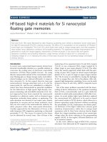
The same conclusions can be drawn if we take a closer
look at Figure 4. A wavelet block from the DWT-transformed
current fr ame is taken as the current block, while the ODWT
transformed reference frame is taken as the reference. For all
possible displacements (dx, dy), the MAD of the prediction
residuals is computed by compensating only the HL sub-
band family, that is, the one that we argue being suitable
for estimating the horizontal displacement. In Figure 4(a),

the global minimum of this function is equal to zero and is
located at (0, 0). In addition, around the global minimum
there is a region that is elongated in the vertical direction,
which is characterized by low values of the MAD. Let u s now
consider a sequence of two images, one obtained from the
other through translation of the vector (dx

, dy

) = (10, 5)
(see Figure 4(b)). Considering a wavelet block on the current
image, Figure 4 shows the MAD value for all the possible dis-
placements. A full search algorithm would identify the global
minimum M. Our algorithm starts f rom point A(0, 0) and
proceeds horizontally both ways to search for the minimum
(B). If dy

is not too large, the horizontal search finds its op-
timum in the elongated valley centered on the global mini-
mum, therefore the horizontal component is estimated quite
accurately. The vertical component can now be estimated
without problems using the LH family subbands. In conclu-
sion, coarsely initializing the algorithm with a full search pro-
vides better results in case of large dy

displacement without
significantly affecting the computational complexity.
M. Tagliasacchi et al. 7
−15
−10

−5
0
5
10
15
dy
−15 −10 −50 51015
dx
(a)
−15
−10
−5
0
5
10
15
dy
−15 −10 −50 51015
dx
AB
M
(b)
Figure 4: Error surface as a function of the candidate motion vector (dx, dy): (a) global minimum in (0, 0); (b) global minimum in (15, 5).
HL
1
HH
1
HL
2
HH

2
LH
1
LH
2
HL
3
HH
3
LL
3
LH
3
(a)
HL
1
HH
1
HL
2
HH
2
LH
1
LH
2
HL
3
HH
3

LL
3
LH
3
(b)
HL
1
HH
1
HL
2
HH
2
LH
1
LH
2
HL
3
HH
3
LL
3
LH
3
(c)
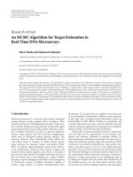
Figure 5: Motion field assigned to a 16 × 16 wavelet block: (a) one vector per wavelet block; (b) four vectors per wavelet block; (c) further
splitting of the wavelet subblock.
2.2. Variable size block matching
As described so far, the FIBME fast search algorithm works

with wavelet blocks of fixed sizes. We propose a simple ex-
tension that allows to adopt blocks of variable sizes by gener-
alizing the HVSBM (hierarchical variable size block match-
ing) [23] algorithm to work in the wavelet domain. Let us
consider a three-level wavelet decomposition and a wavelet
block of size 16
× 16 (refer to Figure 5(a)). In the fixed size
implementation, only one motion vector is assigned to each
wavelet block. If we focus on the lowest frequency subband,
the wavelet block covers a 2
× 2 pixel area. Splitting this area
into four and taking the descendants of each element, we
generate four 8
× 8 wavelet blocks, which are the offspring
of the 16
× 16 parent block (see Figure 5(b)). Block match-
ing is performed on those smaller wavelet blocks to estimate
four distinct motion vectors. In that figure, all the elements
that have the same color are assigned the same motion vector.
Like in HVSBM, we build a quadtree-like structure where in
each node we store the motion vector, the rate R needed to
encode the motion vector and the distortion D (MAD). A
pruning algorithm is then used to select the optimal splitting
configuration for a given bitrate budget [23]. The number B
of different block sizes relative to the wavelet block size N and
the wavelet decomposition level K is
B
= log
2


N
2
K

+ 1 (17)
that corresponds to the block sizes:

N
2
i
×
N
2
i

, i = 0, , B − 1. (18)
If we do not want to be forced to work with fixed size
blocks, we need to have at least two different block sizes. For
8 EURASIP Journal on Applied Signal Processing
example, with B = 2, we have
log
2

N
2
K

> 1 =⇒
N
2

K
> 2 =⇒ N>2
K+1
. (19)
Having fixed K, the previous equation sets a lower bound
on the size of the smallest wavelet block. By setting N
= 16
and K
= 3, three different block sizes are allowed: 16 × 16,
8
× 8, and 4 × 4. We can take this approach one step fur-
ther in order to overcome the lower bound. If N
= 2
K
or
if we have already split the wavelet block in such a way that
there is only one pixel in the LL
K
subband, further split can
be performed according to the above scheme. In order to
provide a motion field of finer granularity, we can still as-
sign a new motion vector to each subband LH
K
, HL
K
, HH
K
,
plus the refined version of LL
K

alone. This way we produce
four children motion vectors, as shown in Figure 5(c). In this
case, the motion vector shown in subband HL
3
is the same
one used for compensating all of the coefficients in subbands
HL
3
, HL
2
,andHL
1
. The same figure shows a further splitting
step perfor med on the wavelet block of the LH
3
subband. In
fact, the splitting can be iterated at lower scales, by assigning
one motion vector to each one-pixel subblock at level K
− 1
(in subband LH
2
in this example). Figure 5(c) shows that the
wavelet block with roots on the blue pixel (in the top-left po-
sition) in subband LH
3
, is split into four subblocks in the LH
2
subband. These refinement steps allow us to compensate el-
ements in different subbands with different motion vectors
that correspond to the same spatial location. We need to em-

phasize that this last splitting step makes the difference be-
tween spatial domain variable size block matching and the
proposed algorithm. In fact, in the latter case it is possible
to compensate the same spatial region with separate motion
vectors, according to the local texture orientation. Following
this simple procedure, we can generate subblocks of arbitrary
size in the wavelet domain.
2.3. Scalable coding of motion vec tors
In both t+2D and 2D+t, wavelet-based video codec SNR scal-
ability is achieved by truncating the embedded representa-
tion of the wavelet coefficients. In this way, only the texture
information is scaled, while the motion information is loss-
less encoded, thus occupying a fixed amount of the bit bud-
get decided at encoding time and unaware of the decoding
bitrate. This fact has two major drawbacks. First, the video
sequence cannot be encoded at a target bitrate lower than the
one necessary to lossless encode the motion vectors. Second,
no optimal tradeoff between motion and residuals bit budget
can be computed.
Recently, it has been demonstrated [26] that in the case
of open-loop wavelet-based video coders it is possible to use
a quantized version of the motion field dur ing decoding to-
gether w ith the residual coefficients computed at the encoder
with the lossless version of the motion. A scalable representa-
tion of the motion is achieved in [26] by coding the motion
field as a two-component image u sing a JPEG2000 scheme.
This is possible as long as the motion vectors are disposed on
a regular lattice, as it is the case for fixed size block matching
or deformable meshes using equally spaced control points.
In this section, we introduce an algorithm able to build a

scalable representation of the motion vectors which is specifi-
cally designed to work with blocks of variable sizes produced
in output by the motion estimation algorithm presented in
Sections 2.1 and 2.2.
Block sizes range from N
max
× N
max
to N
min
× N
min
and
they tend to be smaller in reg ions characterized by complex
motion. Neighboring blocks usually manifest a high degree
of similarity, therefore a coding algorithm able to reduce
their spatial redundancy is needed. In the standard imple-
mentation of HVSBM [23], a simple nearest neighbor pre-
dictor is used for this purpose. Although it achieves a good
lossless coding efficiency, it does not provide a scalable rep-
resentation. The proposed algorithm aims at achieving the
same performance when working in lossless mode allowing
at the same time a scalable representation of the motion in-
formation.
In order to tackle spatial redundancy, a multi-resolution
pyramid of the motion field is built in a bottom-up fashion.
As shown in Figure 6, variable size block matching generates
a quadtree-like representation of the motion model. At the
beginning of the algorithm, only the leaf nodes are assigned
with a value, representing the two components of the mo-

tion vector. For each component, we compute the value of
the node as a simple average of its four offspring. Then we
code each offspring as the difference between each value and
its parent. We iterate these steps further up the motion vec-
tor tree. The root node contains an average of the motion
vectors over the whole image. Depending on the size of the
image and N
min
, the root node might have fewer than four
offspring.
Figure 6 illustrates a toy example that clarifies this multi-
resolution representation. The motion vector components
are the numbers indicated just below each leaf node. The av-
erages computed on intermediate nodes are shown in grey,
while the values to be encoded are written in bold typeface.
The same figure also shows the labeling convention we use:
each node is identified by a pair (i, d), where d represents the
depth in the tree while i is the index number starting from
zero of the nodes at a given depth. Since the motion field
usually exhibits a certain amount of spatial redundancy, the
leaf nodes are likely to have a smaller absolute values. In other
words, walking down from the root to the leaves, we can ex-
pect the same sort of energy decay that is specific of wavelet
coefficients across subbands following parent-children rela-
tionships. This fact suggested us that the same ideas under-
pinning wavelet-based image coders could be exploited here.
Specifically, if an intermediate node is insignificant w ith re-
spect with a given threshold, then it is likely that its de-
scendants are also insignificant. This is the reason why the
proposed algorithm inherits some of the basic concepts of

SPIHT [2] (set partitioning in hierarchical trees).
Before detailing the steps of the algorithm, it is impor-
tant to point out that, in the quadtree representation that we
have built so far, the node values should be multiplied by a
weighting factor that depends on their depth in the tree. Let
us consider only one node and its four offspring. If we wish to
achieve a lossy representation of the motion field, these nodes
M. Tagliasacchi et al. 9
00 00
0,1 1,1 2,1 3,1
2222
0
−13−20 1 −13
2 1502312
0,2 1,2 2,2 3,2 4,2 5,2 6,2 7,2
−10 1 0
0,3 1,3 2,3 3,3
12 34
2
0,0
2
Motion vector difference
Node coordinates
Motion vector component
Average of children motion vectors
Δmv
x
i,d
mv
x

mv
avg
Figure 6: Quadtree-like representation of the motion model generated by the variable size block matching algorithm.
will be quantized. If we make an error in the parent node,
that will badly affec t its offspring, while the same error will
have fewer consequences if one of the children is involved. If
we use the mean squared error as a distortion measure, the
parent node needs to be multiplied by a factor of 2, in such a
way that errors are weighted equally and the same quantiza-
tion step sizes can be used regardless of the node depth.
The proposed algorithm encodes the nodes of the
quadtree from top to bottom starting from the most signif-
icant bitplane. As in SPIHT, the algorithm is divided into
a sorting pass that identifies which nodes are significant
with respect to a given threshold, and a refinement pass
that refines the nodes already found significant in the pre-
vious steps. There are four lists that are maintained both at
the encoder and the decoder, which allow to keep track of
each node status. The L IV (list insignificant vectors) con-
tains those nodes that have not been found significant yet.
The LIS (list insignificant sets) represents those nodes whose
descendants are insignificant. On the other hand, LSV (list
significant vectors) and LSS (list significant sets) contain ei-
ther nodes found significant or whose descendants are signif-
icant. A node can be moved from LIV to LIS and from LIS to
LSS, but not vice versa. Only the nodes in the LSV are refined
during the refinement pass. The follow ing notation is used:
(i) P(i, d): coordinates of parent node of node i at depth
d;
(ii) O(i, d): set of coordinates of all offspring of node i at

depth d;
(iii) D(i, d): set of coordinates of all descendants of node i;
at depth d;
(iv) H(0, 0): coordinate of the quadtree root node.
The algorithm is described in detail by pseudocode listed in
Algorithm 1. Note that

d keeps track of the depth of the cur-
rent node. This way instead of scaling by a factor of 2 all the
intermediate nodes with respec t to their offspring, the signif-
icance test is carried out at bitplane n +

d, that is, S
n+

d
(i

d
,

d).
As for SPIHT, encoding and decoding use the same algo-
rithm, where the word output is substituted by input at the
decoder side. The symbols emitted by the encoder are arith-
metic coded.
The bitstream produced by the proposed algorithm is
completely embedded, in such a way that it is possible to
truncate it at any point and obtain a quantized representation
of the motion field. In [26], it is proved that for small dis-

placement errors, there is a linear relation between the MSE
(mean square error) of the quantized motion field parame-
ters (MSE
W
) and the MSE of the prediction residue (MSE
r
):
MSE
r
= k
ψ
x
+ ψ
y
2
MSE
W
, (20)
where the motion sensitivity factors are defined as
ψ
x
=
1
(2π)
2

S
f
(ω)ω
2

x
dω,
ψ
y
=
1
(2π)
2

S
f
(ω)ω
2
y
dω,
(21)
where S
f
(ω) is the power spectrum of the current frame
f (x, y). Using this result it is possible to estimate a priori
the optimal bit allocation between motion information and
residual coefficients [26]. Informally speaking, at low bitrates
the motion field can be heavily quantized in order to reduce
its bit budget and save bits to encode residual information.
On the other hand, at high bitrates the motion field is usu-
ally sent lossless as it occupies a small fraction of the overall
target bitrate.
2.4. Motion vectors and spatial scalability
A spatially scalable video codec is able to deliver a sequence
at a lower resolution than the original one in order to fit

the receiving device display capabilities. Wavelet-based video
coders address spatial scalability in a st raightforward way. At
the end of spatio-temporal analysis each frame of a GOP of
size T represents a temporal subband further decomposed
into spatial subbands up to level K. Each GOP thus consists
10 EURASIP Journal on Applied Signal Processing
(1) Initialization:
(1.1) output msb
= n =log
2
max
(i,d)
(c
i,d
)
(1.2) output max depth = max(d)
(1.3) set the LLS and the LSV as empty lists add H(0,0) to the LIV and to the LIS.
(2) Sorting pass
(2.1) set

d = 0, set i
d
= 0(d = 0, 1, ,max depth)
(2.2) if 0
≤ n +

d ≤ msb do:
(2.2.1) if entry (i

d

,

d)isintheLIVdo:
(i) output S
n+

d
(i

d
,

d)
(ii) if S
n+

d
(i

d
,

d) = 1thenmove(i

d
,

d)toLSVandoutputthesignofc
i


d
,

d
(2.3) if entry (i

d
,

d)isintheLISdo:
(2.3.1) if n +

d<msb do:
(i) S
D
= 0
(ii) for h
=

d +1tomax depth do:
–foreach(j, h)
∈ D(i

d
,

d), if S
n+h
( j, h) = 1 then S
D

= 1
(iii) output S
D
(iv) if S
D
= 1thenmove(i

d
,

d) to LSS, add each (k, l) ∈ O(i

d
,

d) to the LIV and to the LIS, increment

d
by 1, and go to Step (2.2)
(2.4) if entry (i

d
,

d) is in the LSS the increment

d by 1 and go to Step (2.2).
(3) Refinement pass
(3.1) if 0
≤ n +


d ≤ msb do:
(i) if entry (i

d
,

d) is in t he LSV and was not included during the last sorting pass, then output the nth most signifi-
cant bit of
|c
i,

d
|
(3.2) if

d ≥ 1do
(i) increment i

d
by 1
(ii) if (i

d
,

d) ∈ O(P(i

d
−1,


d
)) then go to Step (2.2); otherwise decrement

d by 1 and go to Step (3).
(4) Quantization step update:decrementn by 1 and go to Step (2).
Algorithm 1: Pseudocode of the proposed scalable motion vector encoding algorithm.
of the following subbands: LL
t
i
, LH
t
i
, HL
t
i
, HH
t
i
with spatial
subband index i
= 1, , K and temporal subband index t =
1, , T. Let us assume that we want to decode a sequence at a
resolution 2
(k−1)
times lower than the original one. We need
to send only those subbands with i
= k, , K. At the de-
coder side, spatial decomposition and motion-compensated
temporal filtering is inverted in the synthesis phase. It is a de-

coder task to adapt the full resolution motion field to match
the resolution of the received subbands.
In this section we compare analytically the following two
approaches:
(a) the original motion vectors are truncated and rounded
in order to match the resolution of the decoded se-
quence,
(b) the original motion vectors are retained, while a full
resolution sequence is interpolated starting from the
received subbands.
The former implementation tends to be computationally
simpler while not as efficient as the latter in terms of coding
efficiency as it will be demonstrated in the following. Fur-
thermore, this is the technique adopted in the MC-EZBC [5]
reference software, used as a benchmark in Section 3.
Let us concentrate our attention on a one-dimensional
discrete signal x(n) and its translated version by an integer
displacement d, that is, y(n)
= x(n − d). Their 2D counter-
part are the current and the reference frame, respectively. We
arethusneglectingmotioncompensationerrorsduetocom-
plex motion, reflections, and illumination changes. Temporal
analysis is carried out with the lifting implementation of the
Haar transform along the motion trajectory d:
H(n)
=
1
√
2


y(n) − x(n − d)

=
0,
L(n) =
√
2x(n)+H(n + d) =
√
2x(n),
(22)
M. Tagliasacchi et al. 11
L(n)andH(n) are wavelet-transformed and, in the case of
spatial scalability, only a subset of their subbands is sent. If
we scale at half the original resolution, the decoder receives
the following signals:
H
low
(n) = 0,
L
low
(n) =
√
2x
low
(n) =
√
2

x ∗ h(k)


k=2n
.
(23)
Temporal synthesis reconstructs a low resolution approxima-
tion of the original signals:
x
low
(n) =
1
√
2

L
low
(n) − H
low

n +
d
2

=
x
low
(n),
y
low
(n) =
√
2H

low
(n)+x
low

n −
d
2

=
x
low

n −
d
2

.
(24)
We compute the reconstruction error using the spatially low-
pass filtered and subsampled version of the original fra mes
as reference:
e
x
(n) = x
low
(n) − x
low
(n) = 0,
e
y

(n) = y
low
(n) − y
low
(n) = x
low

n −
d
2

−
y
low
(n).
(25)
We derive the solution for scenario (b) first, since we will see
(a) as a particular case.
First, the decoder reconstructs an interpolated version
of the original sequence. This is accomplished by setting to
zero the coefficients of the missing subbands before perform-
ing the wavelet synthesis. It is wor th pointing out that this
is equivalent to estimating the missing samples using the
wavelet scaling function as interpolating kernel. The recon-
structionerrorcanbewrittenas
N/2−1

n=0
e
2

y
=
N−1

n=0
e
2
rec
=
N/2−1

n=0


x
rec
b
(n − d) − y
rec
(n)


2
. (26)
The first equivalence holds as far as we use an orthogonal
transform to reconstruct a full resolution approximation of
the signals.
Figure 7 illustrates how e
rec
(n) is computed starting from

x( n)andy(n). H(z) represents the analysis wavelet low-pass
filter, while G(z) is the synthesis low-pass filter. In the rest of
this paper, we assume that they are Daubechies 9/7 biorthog-
onal filters. As they are nearly orthogonal, (26)issatisfiedin
practice. The reconstructed signal x
rec
(n) is an approxima-
tion of x(n) having the same number of samples. Therefore
motion compensation can use the original motion vector d.
Using the Parseval’s theorem and further manipulating the
expression, the prediction error in (26) becomes (for any odd
displacement d)
N/2−1

n=0
e
2
rec
b
= 2

+π
0


G(ω + π)


2



H(ω)


2


X(ω)


2
dω. (27)
If d is even the error expression is identically equal to zero.
Figure 8 depicts
|G(ω + π)|
2
and |H(ω)|
2
together with their
(x)n
H(z) G(z)
x
rec
(n) e
rec
(n)
−
z
−d
y(n)

H(z) G(z)
z
d
y
rec
(n)
Figure 7: Reconstruction error computation without motion vec-
tor truncation (scenario (b)).
0
0.5
1
1.5
2
2.5
00.511.522.533.5
ω
|H(ω)|
2
|G(ω + π)|
2
|I(ω + π)|
2
|H(ω)|
2
|G(ω + π)|
2
|H(ω)|
2
|I(ω + π)|
2

Figure 8: Frequency responses of the filters cited in the paper.
product. We can conclude that the error depends on the fre-
quency characteristics of the signal and it is close to zero if its
energy is mostly concentrated at low frequencies. Indeed the
approximation we get interpolating with G(ω)isverymuch
similar to the original.
The error in scenario (a) can be derived as a special case
of scenario (b). Since the received signal has lower resolution
than the motion field, vectors are truncated. If the compo-
nents are odd, the y are also rounded to the nearest integer.
The reconstruction error is
N/2−1

n=0
e
2
y
=
N/2−1

n=0




x
low

n − round


d
2

−
y
low
(n)




2
. (28)
In order to find a frequency domain expression for this sce-
nario, we can observe that the operation of truncating and
rounding motion vectors is equivalent to interpolating the
low resolution version received by the decoder with a sample
and hold filter and then applying the full resolution motion
12 EURASIP Journal on Applied Signal Processing
0
0.2
0.4
Error
0.65 0.70.75 0.80.85 0.90.95 1
1.5
2
2.5
Error ratio
Err
a

Err
b
Err
a
/Err
b
Figure 9: Comparison between the (normalized) error in scenario (a) and (b) as a function of the correlation coefficient ρ.
field. As a matter of fact, the error can be expressed as
N/2−1

n=0
e
2
y
=
N−1

n=0
e
2
rec
a
(n)
= 2

+π
0





e
jω
√
2
−
1
√
2




2


H(ω)


2


X(ω)


2
dω
= 2

+π

0


I(ω + π)


2


H(ω)


2


X(ω)


2
dω.
(29)
The equivalence holds because the interpolating sample and
hold filter I(ω) is equivalent to the inverse Haar DWT, where
the low-frequency subband is the subsampled signal and the
high-frequency subband coefficients are set to zero. Having
fixed
|H(ω)|
2
, we are unable to state which of the two ap-
proaches is better, that is, has smaller error, since

|I(ω)|
2
is
not greater than
|G(ω)|
2
for all ω (see Figure 2)andwedo
not know the power spectrum of the signal. Nevertheless, if
we assume that most of the energy is concentrated at low fre-
quencies, approach (b) gives better coding efficiency. In fact,
taking the expectation of (27)and(29)withrespecttox(n):
Err
a
= E

N−1

n=0
e
2
rec
a
(n)

=
2

+π
0



I(ω + π



2


H(ω)


2
S
x
(ω)dω,
Err
b
= E

N−1

n=0
e
2
rec
b
(n)

=
2


+π
0


G(ω + π)


2


H(ω)


2
S
x
(ω)dω.
(30)
If we model the signal as an autoregressive process of order
1 with correlation coefficient ρ, the signal power spectrum
S
x
(ω) can be expressed in closed form as
S
x
(ω) =
1 − ρ
2



1 − ρe
jω


2
. (31)
We are now able to evaluate numerically (30). As illustrated
in Figure 9,foranyρ,in[0.7, 1]
2
Err
a
> Err
b
and their ra-
tio is higher for ρ close to 1, meaning that the penalty due
to motion vector truncation with respect to interpolating at
full resolution with G(ω) is greater when the input signal has
energy concentrated in the low-frequency range.
Section 3 validates the results of the formal analysis by
giving experimental evidence about the better coding effi-
ciency achievable without truncating the motion vectors.
3. EXPERIMENTAL RESULTS
In this section, we discuss the overall performance of the
2D+t scalable video codec presented in Section 2 in terms of
complexity and coding efficiency. We emphasize the impact
of each of the coding tools detailed in this paper, in order to
evaluate the best combination of the coding parameters.
As a benchmark, we use the MC-EZBC codec (motion-
compensated embedded zero-block coding) [5] for the t+2D

case, as the proposed 2D+t codec shares some of its func-
tional modules (i.e., spatial and temporal filters, entropy cod-
ing algorithm).
Throughout our simulations, we used the following set
of parameters:
2
Although Figure 9 is zooming on the [0.7, 1] range, the same behavior is
observed in the whole [0, 1] interval.
M. Tagliasacchi et al. 13
(i) sequence spatio-temporal resolution:
– QCIF (176
× 144) at 30 fps: Silent
– CIF (352
× 288) at 30 fps: Mobile & Calendar,
Foreman, Football
– 4CIF (704
× 576) at 60 fps: City, Soccer;
(ii) number of frames: 300;
(iii) spatial wavelet transform: Daubechies 9/7:
–QCIF:K
= 3
–CIF:K
= 3
–4CIF:K
= 4;
(iv) temporal transform: Haar;
(v) GOP size: 16 frames;
(vi) search window: [
−W/2,+W/2]:
–QCIF:[

−16, +16]
–CIF:[
−32, +32]
–4CIF:[
−48, +48];
(vii) motion accuracy: 1/4 pixel;
(viii) block size:
– QCIF and CIF: fixed size 16
× 16, variable size
64
× 64 to 4 × 4
–4CIF:fixedsize32
×32, variable size 128 ×128 to
4
× 4;
(ix) entropy coding: EZBC.
In the first experiment, we compare the proposed fast
motion estimation algorithm (FIBME) (see Section 2.1)with
the computationally demanding full search st rategy. As a ref-
erence, we include the rate-distortion curve obtained with
MC-EZBC. In terms of encoding complexity, the proposed
algorithm allows a speedup factor of the overall encoding
phase equal to 18–19. To this regard, Tabl e 1 shows, for each
sequence, the encoding time normalized with respect to the
encoding time needed when FIBME is used for the same se-
quence. Note that also MC-EZBC uses a fast motion estima-
tion algorithm (HVSBM [23]).
Figure 10 and Tabl e 2 show the rate-distortion perfor-
mance of the proposed 2D+t codec with FIBME with respect
to a full search motion estimation algorithm. In both cases,

blocks of variable sizes are used. From these results we can
conclude that, apart from the Mobile & Calendar sequence
and Foreman at high bitrates, the rate-distortion gap between
FIBME and full search remains within the 0 dB–0.3 dB range.
In all of the remaining experiments, the 2D+t codec always
uses the FIBME algorithm in the motion estimation phase.
Figure 11 and Table 3 show the object ive PSNR gain that
can be obtained by using blocks of variable sizes with the
FIBME algorithm. It should be noticed that the effective-
ness of this feature depends on the complexity of the scene
to be encoded. The more complex the motion, the highest
the benefit of using blocks of variable size would be. For rea-
sons of space, we report the results for Foreman and Football.
The other sequences are characterized by a simpler motion,
therefore the coding gain tends to be more limited. In all of
the remaining simulations, blocks of variable sizes are always
used.
Table 1: Normalized encoding time.
Sequence MC-EZBC Full search FIBME
Silent 1.35 19.32 1
Mobile & Calendar 1.80 18.03 1
Foreman 1.60 18.56 1
Football 1.72 19.02 1
City 1.54 18.47 1
Soccer 1.60 19.14 1
Figure 12 and Table 4 show the results of the simula-
tions conducted when the scalable motion coding algorithm
presented in Section 2.3 is introduced. In the 2D+t codec,
both FIBME and blocks of variable sizes are turned on. For
the nonscalable case, motion vectors are encoded as in MC-

EZBC, by arithmetic coding the prediction residue obtained
as the difference between the motion vector and its causal
predictor. We can conclude the following:
(i) when the motion information is scaled, it is possible
to achieve a lower target bitrate. In Figure 12,itcan
be noticed that in the nonscalable case, for the Foot-
ball sequence, the minimum target bitrate is equal to
128 kbps, whereas it is possible to decode at 64 kbps
when the proposed algorithm is used;
(ii) at low bitrates, a P SNR improvement (up to +3 dB)
is obtained by scaling the motion information as a
fraction of the bit budget can be allocated to encode
wavelet residual coefficients;
(iii) at high bitrates, the proposed algorithm causes a lim-
ited coding efficiency loss (less than 0.1 dB) due to the
fact that the lossless representation produced in the
scalable case is not as efficient as in the nonscalable
case. This is the cost associated to the embedded rep-
resentation of the motion information.
Finally, we discuss the effect of truncating the motion
vectors when a sequence is decoded at reduced spatial resolu-
tions. In this case, there is no unique reference for the PSNR
computation [33], since the truncation of motion vectors af-
fects the MCTF synthesis phase. For this reason, in Figure 13
and Tab le 5 , PSNR values are computed using the spatially
downsampled sequence obtained extracting the LL
K
sub-
band from the wavelet spatial analysis. When the sequences
are decoded at reduced frame rate, the frame skipped se-

quence is used as a reference. Experimental subjective results
[33] demonstrated that the relationship between visual qual-
ity and objective PSNR measurements is usually weak, unless
the reference stays the same. For this reason, we also carried
out visual tests in order to assess the effect of motion vec-
tors truncation in terms of visual quality. In Figure 14,itis
possible to see a sample frame from the Mobile & Calendar
sequence where it is clearly visible that motion vector trunca-
tion affects the visual quality of the reconstructed sequence.
The same evidence is also true for all of the other tested se-
quences.
As a final remark, we can see that the proposed codec
has a coding efficiency comparable with the t+2D MC-EZBC
codec at full resolution a nd tends to outperform MC-EZBC
14 EURASIP Journal on Applied Signal Processing
25
30
35
40
45
50
55
Average Y PSNR
256 512 768 1024 1280 1536
Rate (kbps)
t+2D (MC-EZBC)
2D+t-full search
2D+t-FIBME
Silent QCIF@30 fps
(a)

16
18
20
22
24
26
28
30
32
34
36
Average Y PSNR
256 512 768 1024 1280 1536 1792 2048
Rate (kbps)
t+2D (MC-EZBC)
2D+t-full search
2D+t-FIBME
Mobile & Calendar CIF@30 fps
(b)
22
24
26
28
30
32
34
36
38
40
42

Average Y PSNR
256 512 768 1024 1280 1536 1792 2048
Rate (kbps)
t+2D (MC-EZBC)
2D+t-full search
2D+t-FIBME
Foreman CIF@30 fps
(c)
22
24
26
28
30
32
34
36
Average Y PSNR
256 512 768 1024 1280 1536 1792 2048
Rate (kbps)
t+2D (MC-EZBC)
2D+t-full search
2D+t-FIBME
Football CIF@30 fps
(d)
22
24
26
28
30
32

34
36
38
Average Y PSNR
512 1536 2560 3584 4608 5632
Rate (kbps)
t+2D (MC-EZBC)
2D+t-full search
2D+t-FIBME
City 4CIF@60 fps
(e)
24
26
28
30
32
34
36
38
40
Average Y PSNR
512 1536 2560 3584 4608 5632
Rate (kbps)
t+2D (MC-EZBC)
2D+t-full search
2D+t-FIBME
Soccer 4CIF@60 fps
(f)
Figure 10: FIBME versus full search.
M. Tagliasacchi et al. 15

Table 2: Comparison between MC-EZBC (t+2D with HVSBM), 2D+t with full search motion estimation, and 2D+t w ith FIBME.
kbps
MC- 2D+t 2D+t
(c)–(a) (c)–(b)
EZBC (a) FS (b) FIBME (c)
32 — 27.30 27.25 — −0.05
64 30.61 31.59 31.58 0.97
−0.01
128 34.90 35.73 35.71 0.81
−0.02
256 39.56 40.58 40.56 1.00
−0.02
512 45.35 46.17 46.15 0.80
−0.02
768 48.87 49.63 49.62 0.75
−0.01
1024 51.33 51.84 51.83 0.50
−0.01
1536 53.37 53.47 53.46 0.09
−0.01
(a) Silent QCIF@30 fps
kbps
MC- 2D+t 2D+t
(c)–(a) (c)–(b)
EZBC (a) FS (b) FIBME (c)
64 — 17.46 17.07 — −0.39
128 — 20.95 20.54 —
−0.41
256 23.31 24.31 23.76 0.45
−0.55

512 28.02 28.05 27.27
−0.75 −0.78
768 30.34 30.06 29.46
−0.88 −0.60
1024 31.74 31.56 31.05
−0.69 −0.51
1536 33.69 33.52 33.15
−0.54 −0.37
2048 35.27 35.19 34.86
−0.41 −0.33
(b) Mobile & Calendar CIF@30 fps
kbps
MC- 2D+t 2D+t
(c)–(a) (c)–(b)
EZBC (a) FS (b) FIBME (c)
64 — 23.86 23.69 — −0.17
128 — 28.37 28.16 —
−0.21
256 31.29 31.65 31.31 0.02
−0.34
512 34.53 34.82 34.34
−0.19 −0.48
768 36.19 36.55 36.03
−0.16 −0.52
1024 37.56 38.03 37.49
−0.07 −0.54
1536 39.44 39.89 39.38
−0.06 −0.51
2048 40.98 41.49 40.98 0
−0.51

(c) Foreman CIF@30 fps
kbps
MC- 2D+t 2D+t
(c)–(a) (c)–(b)
EZBC (a) FS (b) FIBME (c)
64 — — — — —
128 — 22.83 23.00 — 0.17
256 — 25.59 25.58 —
−0.01
512 27.70 28.26 28.18 0.48
−0.08
768 29.45 29.94 29.81 0.36
−0.13
1024 30.80 31.48 31.32 0.52
−0.16
1536 32.83 33.69 33.51 0.68
−0.18
2048 34.63 35.63 35.40 0.77
−0.23
(d) Football CIF@30 fps
kbps
MC- 2D+t 2D+t
(c)–(a) (c)–(b)
EZBC (a) FS (b) FIBME (c)
256 — 23.48 23.34 — −0.14
512 23.82 26.71 26.52 2.70
−0.19
768 28.16 28.49 28.26 0.10
−0.23
1024 30.13 29.68 29.42

−0.71 −0.26
1536 32.34 31.50 31.22
−1.12 −0.28
2048 33.71 32.73 32.44
−1.27 −0.29
3000 35.19 34.41 34.15
−1.04 −0.26
6000 37.47 37.02 36.85
−0.62 −0.17
(e) City 4CIF@60 fps
kbps
MC- 2D+t 2D+t
(c)–(a) (c)–(b)
EZBC (a) FS (b) FIBME (c)
256 — 24.57 24.97 — 0.40
512 — 27.84 27.65 —
−0.19
768 — 29.42 29.17 —
−0.25
1024 29.61 30.47 30.26 0.65
−0.21
1536 31.84 32.17 31.96 0.12
−0.21
2048 33.09 33.34 33.18 0.09
−0.16
3000 34.73 35.06 34.93 0.20
−0.13
6000 37.65 38.12 37.89 0.24
−0.23
(f) Soccer 4CIF@60 fps

22
24
26
28
30
32
34
36
38
40
42
Average Y PSNR
256 512 768 1024 1280 1536 1792 2048
Rate (kbps)
t+2D (MC-EZBC)
2D+t-FIBME-VSBM
2D+t-FIBME-FSBM
Foreman CIF@30 fps
(a)
22
24
26
28
30
32
34
36
Average Y PSNR
256 512 768 1024 1280 1536 1792 2048
Rate (kbps)

t+2D (MC-EZBC)
2D+t-FIBME-VSBM
2D+t-FIBME-FSBM
Football CIF@30 fps
(b)
Figure 11: FIBME: fixed block sizes versus variable block sizes.
16 EURASIP Journal on Applied Signal Processing
Table 3: FIBME: fixed block sizes (FSBM) versus variable block sizes (VSBM).
kbps
MC- 2D+t FIBME 2D+t FIBME
(c)–(a) (c)–(b)
EZBC (a) FSBM (b) VSBM (c)
64 — — 23.69 — —
128 — — 28.16 — —
256 31.29 28.73 31.31 0.02 2.58
512 34.53 31.99 34.34
−0.19 2.35
768 36.19 34.03 36.03
−0.16 2.00
1024 37.56 35.30 37.49
−0.07 2.19
1536 39.44 37.54 39.38
−0.06 1.84
2048 40.98 39.05 40.98 0 1.93
(a) Foreman CIF@30 fps
kbps
MC- 2D+t FIBME 2D+t FIBME
(c)–(a) (c)–(b)
EZBC (a) FSBM (b) VSBM (c)
64 — — — — —

128 — — 23.00 — —
256 — 24.24 25.58 — 1.34
512 27.70 27.09 28.18 0.48 0.72
1024 30.80 30.57 31.32 0.52 0.75
1536 32.83 32.76 33.51 0.68 0.75
2048 34.63 34.73 35.40 0.77 0.67
(b) Football CIF@30 fps
Table 4: Nonscalable versus scalable motion vectors.
kbps
MC- Nonscal. Scal.
(c)–(a) (c)–(b)
EZBC (a) MV (b) MV (c)
32 — 27.25 27.50 — 0.25
64 30.61 31.58 31.70 1.09 0.12
128 34.90 35.71 35.80 0.90 0.09
256 39.56 40.56 40.60 1.04 0.04
512 45.35 46.15 46.14 0.79
−0.01
768 48.87 49.62 49.60 0.73
−0.02
1024 51.33 51.83 51.79 0.46
−0.04
1536 53.37 53.46 53.40 0.03
−0.06
(a) Silent QCIF@30 fps
kbps
MC- Nonscal. Scal.
(c)–(a) (c)–(b)
EZBC (a) MV (b) MV (c)
64 — 17.07 20.01 — 2.94

128 — 20.54 22.10 — 1.56
256 23.31 23.76 24.90 1.59 1.14
512 28.02 27.27 27.60
−0.42 0.33
768 30.34 29.46 29.45
−0.89 −0.01
1024 31.74 31.05 31.02
−0.72 −0.03
1536 33.69 33.15 33.10
−0.59 −0.05
2048 35.27 34.86 34.80
−0.47 −0.06
(b) Mobile & Calendar CIF@30 fps
kbps
MC- Nonscal. Scal.
(c)–(a) (c)–(b)
EZBC (a) MV (b) MV (c)
64 — 23.69 25.80 — 2.11
128 — 28.16 29.27 — 1.11
256 31.29 31.31 32.01 0.72 0.70
512 34.53 34.34 34.40
−0.13 0.06
768 36.19 36.03 36.02
−0.17 −0.01
1024 37.56 37.49 37.47
−0.09 −0.02
1536 39.44 39.38 39.33
−0.11 −0.05
2048 40.98 40.98 40.93
−0.05 −0.05

(c) Foreman CIF@30 fps
kbps
MC- Nonscal. Scal.
(c)–(a) (c)–(b)
EZBC (a) MV (b) MV (c)
64 — — 24.30 — —
128 — 23.00 25.30 — 2.30
256 — 25.58 26.80 — 1.22
512 27.70 28.18 28.80 1.10 0.62
768 29.45 29.81 30.10 0.65 0.29
1024 30.80 31.32 31.32 0.52 0.00
1536 32.83 33.51 33.49 0.66
−0.02
2048 34.63 35.40 35.35 0.72
−0.05
(d) Football CIF@30 fps
kbps
MC- Nonscal. Scal.
(c)–(a) (c)–(b)
EZBC (a) MV (b) MV (c)
256 — 23.34 25.80 — 2.46
512 23.82 26.52 27.82 4.00 1.30
768 28.16 28.26 28.88 0.72 0.62
1024 30.13 29.42 29.70
−0.43 0.28
1536 32.34 31.22 31.20
−1.14 −0.02
2048 33.71 32.44 32.40
−1.31 −0.04
3000 35.19 34.15 34.09

−1.10 −0.06
6000 37.47 36.85 36.78
−0.69 −0.07
(e) City 4CIF@60 fps
kbps
MC- Nonscal. Scal.
(c)–(a) (c)–(b)
EZBC (a) MV (b) MV (c)
256 — 24.97 26.50 — 1.53
512 — 27.65 28.75 — 1.10
768 — 29.17 29.90 — 0.73
1024 29.61 30.26 30.80 1.19 0.54
1536 31.84 31.96 32.03 0.19 0.07
2048 33.09 33.18 33.15 0.06
−0.03
3000 34.73 34.93 34.90 0.17
−0.03
6000 37.65 37.89 37.85 0.20
−0.04
(f) Soccer 4CIF@60 fps
M. Tagliasacchi et al. 17
25
30
35
40
45
50
55
Average Y PSNR
256 512 768 1024 1280 1536

Rate (kbps)
t+2D (MC-EZBC)
2D+t-nonscalable MV
2D+t-scalable MV
Silent QCIF@30 fps
(a)
16
18
20
22
24
26
28
30
32
34
36
Average Y PSNR
256 512 768 1024 1280 1536 1792 2048
Rate (kbps)
t+2D (MC-EZBC)
2D+t-nonscalable MV
2D+t-scalable MV
Mobile & Calendar CIF@30 fps
(b)
22
24
26
28
30

32
34
36
38
40
42
Average Y PSNR
256 512 768 1024 1280 1536 1792 2048
Rate (kbps)
t+2D (MC-EZBC)
2D+t-nonscalable MV
2D+t-scalable MV
Foreman CIF@30 fps
(c)
22
24
26
28
30
32
34
36
Average Y PSNR
256 512 768 1024 1280 1536 1792 2048
Rate (kbps)
t+2D (MC-EZBC)
2D+t-nonscalable MV
2D+t-scalable MV
Football CIF@30 fps
(d)

22
24
26
28
30
32
34
36
38
Average Y PSNR
512 1536 2560 3584 4608 5632
Rate (kbps)
t+2D (MC-EZBC)
2D+t-nonscalable MV
2D+t-scalable MV
City 4CIF@60 fps
(e)
24
26
28
30
32
34
36
38
Average Y PSNR
512 1536 2560 3584 4608 5632
Rate (kbps)
t+2D (MC-EZBC)
2D+t-nonscalable MV

2D+t-scalable MV
Soccer 4CIF@60 fps
(f)
Figure 12: Nonscalable versus scalable motion vectors.
18 EURASIP Journal on Applied Signal Processing
18
20
22
24
26
28
30
Average Y PSNR
256 512 768 1024
Rate (kbps)
t+2D (MC-EZBC)
2D+t-no MV truncation
2D+t-MV truncation
Mobile & Calendar QCIF@30 fps
(a)
19
20
21
22
23
24
25
26
27
28

29
Average Y PSNR
256 512 768 1024
Rate (kbps)
t+2D (MC-EZBC)
2D+t-no MV truncation
2D+t-MV truncation
Mobile & Calendar QCIF@15 fps
(b)
20
22
24
26
28
30
32
34
36
38
Average Y PSNR
256 512 768 1024
Rate (kbps)
t+2D (MC-EZBC)
2D+t-no MV truncation
2D+t-MV truncation
Foreman QCIF@30 fps
(c)
27
28
29

30
31
32
33
34
35
36
Average Y PSNR
256 512 768 1024
Rate (kbps)
t+2D (MC-EZBC)
2D+t-no MV truncation
2D+t-MV truncation
Foreman QCIF@15 fps
(d)
Figure 13: Effect of motion vector truncation.
(a) (b)
Figure 14: Effect of motion vector truncation. Mobile & Calendar, QCIF@30 fps—256 kbps: (a) with MV truncation; (b) without MV
truncation.
M. Tagliasacchi et al. 19
Table 5: FIBME: fixed block sizes (FSBM) versus variable block sizes (VSBM).
kbps
MC- MV No MV
(c)–(a) (c)–(b)
EZBC (a) tr unc. (b) trunc. (c)
64 — 18.47 18.53 — 0.06
128 — 22.09 22.78 — 0.69
256 24.41 24.42 25.95 1.54 1.53
512 25.96 25.55 27.83 1.87 2.28
768 26.26 25.88 28.41 2.15 2.53

1024 26.39 26.02 28.65 2.26 2.63
(a) Mobile QCIF@30 fps
kbps
MC- MV No MV
(c)–(a) (c)–(b)
EZBC (a) tr unc. (b) trunc. (c)
64 — 19.84 19.98 — 0.14
128 21.25 22.91 23.46 2.21 0.55
256 25.81 25.15 26.34 0.53 1.19
512 27.06 26.27 27.98 0.92 1.71
768 27.33 26.56 28.40 1.07 1.84
1024 27.42 26.67 28.57 1.15 1.90
(b) Mobile QCIF@15 fps
kbps
MC- MV No MV
(c)–(a) (c)–(b)
EZBC (a) tr unc. (b) trunc. (c)
64 — 25.04 25.16 — 0.12
128 21.84 29.36 30.18 8.34 0.82
256 32.75 31.66 33.50 0.75 1.84
512 34.40 32.97 36 1.60 3.03
768 34.99 33.48 37.16 2.17 3.68
1024 35.25 33.69 37.70 2.45 4.01
(c) Foreman QCIF@30 fps
kbps
MC- MV No MV
(c)–(a) (c)–(b)
EZBC (a) tr unc. (b) trunc. (c)
64 — 27.24 27.53 — 0.29
128 30.28 30.07 30.93 0.65 0.86

256 33.62 31.81 33.43
−0.19 1.62
512 35.06 32.83 35.05
−0.01 2.22
768 35.44 33.07 35.49 0.05 2.42
1024 35.58 33.17 35.68 0.10 2.51
(d) Foreman QCIF@15 fps
at reduced spatio-temporal resolution. Further m ore, the se-
quences decoded with the proposed 2D+t codec are not af-
fected by blocking artifacts that appear in the MC-EZBC
codec, thus improving the subjective qualit y when they at-
tain the same objective performance.
4. CONCLUSIONS
In this paper, we present a fully scalable 2D+t video codec,
where we introduced novel algorithms in the motion estima-
tion and signaling part. The proposed fast motion estima-
tion algorithm is able to achieve good coding efficiency at a
fraction of the computational complexity of a full search ap-
proach. The scalable representation of motion information
improves the objective and subjective quality of sequences
decoded at low bitrates. Our current research activities in
this area focus on the study of rate-distortion optimal mo-
tion modeling in wavelet-based 2D+t video coding schemes.
REFERENCES
[1] D. Taubam and M. W. Marcellin, JPEG2000: Image Compres-
sion Fundamentals, Standards and Practice, Kluwer Academic,
Boston, Mass, USA, 2002.
[2] A. Said and W. A. Pearlman, “A new, fast, and efficient im-
age codec based on set partitioning in hierarchical trees,”
IEEE Transactions on Circuits and Systems for Video Technol-

ogy, vol. 6, no. 3, pp. 243–250, 1996.
[3] S T. Hsiang and J. W. Woods, “Embedded image coding using
zeroblocks of subband/wavelet coefficients and context mod-
eling,” in Proceedings of IEEE International Symposium on Cir-
cuits and Systems (ISCAS ’00), vol. 3, pp. 662–665, Geneva,
Switzerland, May 2000.
[4] J. Xu, Z. Xiong, S. Li, and Y Q. Zhang, “Three-dimensional
embedded subband coding with optimized truncation (3-
DESCOT),”Applied and Computational Harmonic Analysis,
vol. 10, no. 3, pp. 290–315, 2001.
[5] P. Chen and J. W. Woods, “Bidirectional MC-EZBC with lift-
ing implementation,” IEEE Transactions on Circuits and Sys-
tems for Video Technology, vol. 14, no. 10, pp. 1183–1194, 2004.
[6] A. Secker and D. Taubman, “Lifting-based invertible motion
adaptive transform (LIMAT) framework for highly scalable
video compression,” IEEE Transactions on Image Processing,
vol. 12, no. 12, pp. 1530–1542, 2003.
[7] G.Pau,C.Tillier,B.Pesquet-Popescu,andH.Heijmans,“Mo-
tion compensation and scalability in lifting-based video cod-
ing,” Signal Processing: Image Communication,vol.19,no.7,
pp. 577–600, 2004.
[8] J R. Ohm, “T hree-dimensional subband coding with motion
compensation,” IEEE Transactions on Image Processing, vol. 3,
no. 5, pp. 559–571, 1994.
[9] Y. Andreopoulos, A. Munteanu, J. Barbarien, M. van der
Schaar, J. Cornelis, and P. Schelkens, “In-band motion com-
pensated temporal filtering,” Signal Processing: Image Commu-
nication, vol. 19, no. 7, pp. 653–673, 2004.
[10] Y. Wang, S. Cui, and J. E. Fowler, “3D video coding using
redundant-wavelet multihypothesis and motion-compensated

temporal filtering,” in Proceedings of IEEE International Con-
ference on Image Processing (ICIP ’03), vol. 2, pp. 755–758,
Barcelona, Spain, September 2003.
[11] H W. Park and H S. Kim, “Motion estimation using low-
band-shift method for wavelet-based moving-picture coding,”
IEEE Transactions on Image Processing, vol. 9, no. 4, pp. 577–
587, 2000.
[12] J. C. Ye and M. van der Schaar, “Fully scalable 3D overcomplete
wavelet video coding using adaptive motion compensated
temporal filtering,” in Visual Communications and Image Pro-
cessing (VCIP ’03), T. Ebrahimi and T. Sikora, Eds., vol. 5150 of
20 EURASIP Journal on Applied Signal Processing
Proceedings of SPIE, pp. 1169–1180, Lugano, Switzerland, July
2003.
[13] S. Mallat, A Wavelet Tour of Signal Processing, Academic Press,
San Diego, Calif, USA, 1998.
[14] N. Mehrseresht and D. Taubman, “A flexible structure for fully
scalable motion compensated 3D-DWT with emphasis on the
impact of spatial scalability,” submitted to IEEE Transactions
on Image Processing.
[15] N. Mehrseresht and D. Taubman, “An efficient content-
adaptive motion compensated 3D-DWT with enhanced spa-
tial and temporal scalability,” submitted to IEEE Transactions
on Image Processing.
[16] ITU-T, Information technology—Coding of audio-visual
objects—Part 10: Advanced video coding, May 2003, ISO/IEC
International Standard 14496-10:2003.
[17] D. Maestroni, A. Sarti, M. Tagliasacchi, and S. Tubaro, “Fast
in-band motion estimation with variable size block matching,”
in Proceedings of IEEE International Conference on Image Pro-

cessing (ICIP ’04), vol. 4, pp. 2287–2290, Singapore, October
2004.
[18] D. Maestroni, A. Sarti, M. Tagliasacchi, and S. Tubaro, “Scal-
able coding of variable size blocks motion vectors,” in Pro-
ceedings of IEEE International Conference on Image Processing
(ICIP ’04), vol. 2, pp. 1333–1336, Singapore, October 2004.
[19] D. Maestroni, A. Sarti, M. Tagliasacchi, and S. Tubaro,
“Wavelet-based video coding: optimal use of motion informa-
tion for the decoding of spatially scaled video sequences,” in
Proceedings of the 12th European Signal Processing Conference
(EUSIPCO ’04), Vienna, Austria, September 2004.
[20] Y. Andreopoulos, A. Munteanu, G. Van der Auwera, P.
Schelkens, and J. Cornelis, “A new method for complete-to-
overcomplete discrete wavelet transforms,” in Proceedings of
the 14th International Conference on Digital Signal Processing
(DSP ’02), vol. 2, pp. 501–504, Santorini, Greece, July 2002.
[21] Y. Andreopoulos, M. van der Schaar, A. Munteanu, J. Bar-
barien, P. Schelkens, and J. Cornelis, “Fully-scalable wavelet
video coding using in-band motion compensated temporal
filtering,” in Proceedings of IEEE International Conference on
Acoustics, Speech, and Signal Processing (ICASSP ’03), vol. 3,
pp. 417–420, Hong Kong, China, April 2003.
[22] W. Cai and M. Adjouadi, “An efficient approach of fast motion
estimation and compensation in wavelet domain video com-
pression,” in Proceedings of IEEE International Conference on
Acoustics, Speech, and Signal Processing (ICASSP ’04), vol. 2,
pp. 977–980, Montreal, Quebec, Canada, May 2004.
[23] S J. Choi and J. W. Woods, “Motion-compensated 3-D sub-
band coding of video,” IEEE Transactions on Image Processing,
vol. 8, no. 2, pp. 155–167, 1999.

[24] R. Xiong, F. Wu, S. Li, Z. Xiong, and Y Q. Zhang, “Exploiting
temporal correlation w ith adaptive block-size motion align-
ment for 3D wavelet coding,” in Visual Communications and
Image Processing 2004, vol. 5308 of Proceedings of SPIE,pp.
144–155, San Jose, Calif, USA, January 2004.
[25] D. Taubman and A. Secker, “Highly scalable video compres-
sion with scalable motion coding,” in Proceedings of IEEE In-
ternational Conference on Image Processing (ICIP ’03), vol. 3,
pp. 273–276, Barcelona, Spain, September 2003.
[26] A. Secker and D. Taubman, “Highly scalable video compres-
sion with scalable motion coding,” IEEE Transactions on Image
Processing, vol. 13, no. 8, pp. 1029–1041, 2004.
[27] J. Barbarien, A. Munteanu, F. Verdicchio, Y. Andreopoulos, J.
Cornelis, and P. Schelkens, “Scalable motion vector coding,”
Electronics Le tters, vol. 40, no. 15, pp. 932–934, 2004.
[28] G. Boisson, E. Francois, and C. Guillemot, “Accuracy-scalable
motion coding for efficient scalable video compression,” in
Proceedings of IEEE International Conference on Image Process-
ing (ICIP ’04), vol. 2, pp. 1309–1312, Singapore, October 2004.
[29] R. Xiong, J. Xu, F. Wu, S. Li, and Y Q. Zhang, “Layered motion
estimation and coding for fully scalable 3D wavelet video cod-
ing,” in Proceeding of IEEE International Conference on Image
Processing (ICIP ’04), vol. 4, pp. 2271–2274, Singapore, Octo-
ber 2004.
[30] B. D. Lucas and T. Kanade, “An iterative image registration
technique with an application to stereo vision,” in Proceed-
ings of the 7th International Joint Conference on Artificial Intel-
ligence (IJCAI ’81), pp. 674–679, Vancouver, BC, Canada, Au-
gust 1981.
[31] B. K. P. Horn and B. G. Schunck, “Determining optical flow,”

Artificial Intelligence, vol. 17, no. 1–3, pp. 185–203, 1981.
[32] M. A. Tekalp, Digital Video Processing, Prentice-Hall Signal
Processing Series, Prentice-Hall, Upper Saddle River, NJ, USA,
1995.
[33] U. Benzler and M. Wien, “Results of SVC CE3 (Quality
Evaluation),” ISO/IEC JTC1/SC29/WG11 MPEG Document
M10931, July 2004.
M. Tagliasacchi born in 1978, received the
“Laurea” degree (2002, cum Laude) in com-
puter systems engineering from Politec-
nico di Milano, Italy. He is currently work-
ing toward the Ph.D. degree at Politec-
nico di Milano. During 2004, he was Vis-
iting Scholar at University of California at
Berkeley. His research interests include dis-
tributed video coding, scalable video cod-
ing, wavelet-based video coding, and local-
ization of acoustic sources.
D. Maestroni received the “Laurea” de-
gree in communication systems engineering
from Politecnico di Milano, Italy, in 2003.
During 2004, he collaborated with Politec-
nico di Milano and Telecom Italia Lab in
the research activities on scalable video cod-
ing within MPEG. His thesis work and
further research activities concern wavelet-
based scalable video coding.
S. Tubaro born in 1957, completed his stud-
ies in electronic engineering at the “Politec-
nico d i Milano,” Italy, in 1982. He then

joined the “Dipartimento di Elettronica e
Informazione” of the “Politecnico di Mi-
lano,” first as a Researcher of the National
Research Council, then (in November 1991)
as an Associate Professor, and from Decem-
ber 2004 as a Full Professor. In the first
years of activities, he worked on problems
related to speech analysis; motion estimation/compensation for
video analysis/coding, and vector quantization applied to hybrid
video coding. In the past few years, his research interests have fo-
cused on image and video analysis for the geometric and radio-
metric modeling of 3D scenes, advanced algorithms for video cod-
ing and sound processing. He authored more than 150 scientific
publications on international journals and congresses. He coau-
thored two books on digital processing of video sequences. He
M. Tagliasacchi et al. 21
is also a co-author of se veral patents relative to image processing
techniques. He coordinates the research activities of the image and
sound processing group (ISPG) at the “Dipartimento di Elettronica
e Informazione” of the “Politecnico di Milano” that is involved in
several research programs funded by industrial partners, the Italian
Government and by the European Commission.
A. Sarti born in 1963, received the “Laurea”
degree (1988, cum Laude) and the Ph.D.
(1993) in electrical engineering, from the
University of Padua, Italy. He completed his
graduate studies at the University of Califor-
nia at Berkeley. In 1993, he joined the Di-
partimento di Elettronica e Informazione of
the Politecnico di Milano, where he is now

an Associate Professor. His current research
interests are in the area of digital signal pro-
cessing, with particular focus on computer vision, image and sound
processing.