Báo cáo hóa học: " Space-Time Joint Interference Cancellation Using Fuzzy-Inference-Based Adaptive Filtering Techniques in Frequency-Selective Multipath Channels" potx
Bạn đang xem bản rút gọn của tài liệu. Xem và tải ngay bản đầy đủ của tài liệu tại đây (933.17 KB, 17 trang )
Hindawi Publishing Corporation
EURASIP Journal on Applied Signal Processing
Volume 2006, Article ID 62052, Pages 1–17
DOI 10.1155/ASP/2006/62052
Space-Time Joint Interference Cancellation Using
Fuzzy-Inference-Based Adaptive Filtering
Techniques in Frequency-Selective
Multipath Channels
Chia-Chang Hu,
1
Hsuan-Yu Lin,
1
Yu-Fan Chen,
2
and Jyh-Horng Wen
1, 3
1
Department of Electrical Engineering, National Chung Cheng University, Min-Hsiung, Chia-Yi 621, Taiwan
2
Department of Communications Engineering, National Chung Cheng University, Min-Hsiung, Chia-Yi 621, Taiwan
3
Institute of Communication Engineering, National Chi Nan University, Puli, Nantou 545, Taiwan
Received 7 March 2005; Revised 29 May 2005; Accepted 19 July 2005
Recommended for Publication by Helmut Bolcskei
An adaptive minimum mean-square error (MMSE) array receiver based on the fuzzy-logic recursive least-squares (RLS) algorithm
is developed for asynchronous DS-CDMA interference suppression in the presence of frequency-selective multipath fading. This
receiver employs a fuzzy-logic control mechanism to perform the nonlinear mapping of the squared error and squared error
variation, denoted by (e
2
,Δe
2
), into a forgetting factor λ. For the real-time applicability, a computationally efficient version of
the proposed receiver is derived based on the least-mean-square (LMS) algorithm using the fuzzy-inference-controlled step-size
μ. This receiver is capable of providing both fast convergence/tracking capability as well as small steady-state misadjustment as
compared with conventional LMS- and RLS-based MMSE DS-CDMA receivers. Simulations show that the fuzzy-logic LMS and
RLS algorithms outperform, respectively, other variable step-size LMS (VSS-LMS) and variable forgetting factor RLS (VFF-RLS)
algorithms at least 3 dB and 1.5 dB in bit-error-rate (BER) for multipath fading channels.
Copyright © 2006 Hindawi Publishing Corporation. All rights reserved.
1. INTRODUCTION
Direct-sequence code-division multiple access (DS-CDMA),
a specific form of spread-spectrum tr ansmission, has been
adopted as the multiaccess technology for nonorthogonal
transmission in the third-generation (3G) mobile cellular
systems, such as wideband CDMA (W-CDMA) or multi-
carrier CDMA (MC-CDMA). This sort of the code-division
multiaccess techniques requires no time or frequency coor-
dination among the mobile stations. However, the so-called
near-far problem and the multipath fading are the major
impediments to maintain reliable communication links in
CDMA systems.
It is well known that an adaptive minimum mean-square
error (MMSE) linear receiver [1] has immunit y to the near-
far problem and the interference floor in performance exhib-
ited by the conventional matched filter reception. In addi-
tion, a linear MMSE receiver can be implemented as an adap-
tive tapped delay line (TDL), analogous to a linear equalizer,
with a relatively low complexity. However, the computation
of the MMSE solution involves the calculation of the inverse
of the input autocorrelation matrix, which costs a complex-
ity of O((MN)
3
). Here M denotes the size of the MMSE re-
ceiving arr ay and N is the processing gain of the CDMA sys-
tem so that MN indicates the number of tap weights of the
linear MMSE filter. This cost is even more expensive when
the linear MMSE receiver operates in a nonstationary mul-
tipath environment. In practice, the filter-coefficient vector
of the MMSE-type receiver can be obtained from the train-
ing sequence and the received signal by means of conven-
tional adaptive filtering techniques, such as the least-mean-
square (LMS) [2] and the recursive least-squares (RLS) [3]
approaches. The LMS provides simple implementation but
suffers from slow convergence, while, on the other hand, the
RLS converges much faster as compared with the LMS, but it
possesses more computational complexity. The drawback of
slow convergence of an LMS-based algorithm, due to its de-
pendence on the eigenvalue spread, is overcome in an RLS
algorithm [3] by replacing the gradient step-size μ with a
gain matrix, denoted by R
−1
x
[n], at the nth iteration. In [4],
2 EURASIP Journal on Applied Signal Processing
Honig et al. proposed an adaptive blind LMS implementa-
tion of the MMSE-type receiver based on the concept of the
constrained minimum output energy (CMOE) for multiuser
detection. An adaptive blind RLS version of the MMSE re-
ceiver was presented in [5] by Poor and Wang In [5], the pro-
posed rotation-based QR-RLS algorithms for both the blind
adaptation mode and the decision-directed adaptation mode
were developed and implemented efficiently.
In recent years, the concept of fuzzy logic is used in
many different senses. Fuzzy logic can be treated as a tool
for embedding structured human knowledge into workable
algorithms. In a wider sense, fuzzy logic is a fuzzy set the-
ory of classes with unsharp or fuzzy boundaries. Systems
designed and developed utilizing fuzzy-logic methods have
been shown to be more efficient than those based on conven-
tional approaches [6]. Notably, a fuzzy-logic controller (FLC)
has been applied successfully to the fuzzy-neural scheme
for on-line system identification [7] and the strength-based
power control strategy in wireless multimedia cellular sys-
tems [8, 9]. In principle, FLC provides an adaptation mech-
anism that converts the linguistic control strategy based on
the charac teristics of mobile radio channels into an adaptive
parameter-control str ategy. By using the defuzzification, the
fuzzy control decisions are converted to a crisp control com-
mand which is used to adjust properly the level of the param-
eter of interest. To improve the FLC performance, the use of
a fuzzy proportional-plus-integral ( PI) control is addressed
in [10].
In the present paper, an adaptive robust MMSE arr ay-
receiver is proposed based on a fuzzy-logic controlled LMS or
RLS algorithm for space-time joint asynchronous DS-CDMA
signals. The FLC system is employed to perfor m the non-
linear mapping of the input variables into a scalar adapta-
tion step-size μ of the LMS algorithm or a forgetting fac-
tor λ of the RLS algorithm in response to the channel vari-
ation. Note that the input variables of the FLC system may
include the error signal, duration of training, squared error,
input power, and any other useful variables. Owing to the
flexibility and richness of the fuzzy-inference control system,
it may produce many different mappings that are especially
suitable for applications in nonlinear and time-varying cel-
lular systems. In [11], the behavior of different adaptive LMS
algorithms with the fuzzy step size is analyzed. Experimental
results show that the fuzzy step-size LMS (FSS-LMS) algo-
rithms proposed by the author in [11] possess superior con-
vergence characteristics than other existing variable step-size
LMS (VSS-LMS) approaches [12, 13]. In particular, the per-
formance of the FSS-LMS system with two inputs of e
2
and
N
T
is noticeable, where e
2
is the squared error and N
T
de-
notes the duration of training. Unfortunately, the quantity of
N
T
may not be attainable to the category of adaptive blind-
based receivers. In [14], the authors proposed the variable
forgetting factor linear least-squares (VFF-LLS) algorithm to
improve the tracking capability of channel estimation. These
works motivate the development of the linear MMSE CDMA
receiver with a fuzzy-logic controlled two-parameter system
of (e
2
, Δe
2
) instead of (e
2
, N
T
), where Δe
2
[n]
=|e
2
[n]−e
2
[n−
1]| indicates the squared error variation at time n. In other
words, the pair values of (e
2
, Δe
2
) are calculated and fed to
the FLC system to assign an exact value of μ or λ for the cor-
responding adaptive receiver on an iterative basis in order
to improve the convergence characteristic and steady-state
MSE simultaneously. Most of the fuzzy inference rules are
derived by a human expert or extracted from numerical data.
In this paper, we focus attention on the fuzzy rules which ac-
cumulate past experience operating in the practical applica-
tions. Therefore, it seems natural and reasonable to expect
that wireless communication systems with the use of a two-
parameter (e
2
, Δe
2
)-FLC produce better convergence char-
acteristics than those with only single-parameter (e
2
)-FLC.
Furthermore, the pair of (e
2
, Δe
2
) provides the FLC system
with more precise channel dynamic-tracking and adaptation
capability than the pair of (e
2
, N
T
). This is because the “aux-
iliary” parameter Δe
2
offers an effective and robust means
to monitor instantaneous fluctuations of a fast-fading mul-
tipath channel and assists the FLC system in selec ting an ap-
propriate value for μ or λ. It is remarkable that the proposed
FLC-based approaches produce a faster speed of convergence
without trading off the steady-state performance.
Computational requirements of the proposed fuzzy-
logic-controlled LMS and RLS algorithms of the MMSE re-
ceiver, abbreviated as FLC-LMS and FLC-RLS hereafter, are
evaluated in this paper. Slightly additional computational
load is incurred in the fuzzification (table lookup), inference
(MIN, MAX, and PROD operators), and defuzzification pro-
cesses. There is also additional cost which comes from the
preparation of the two input variables, (e
2
, Δe
2
), prior to
the fuzzification process. Fortunately, these operations can be
done very efficiently in the latest range of DSPs which pro-
vide single-cycle multiply and add, table lookup, and com-
parison instructions. The computational load is compared to
other known MMSE CDMA algorithms as well.
The material included in this paper is organized as fol-
lows. In Section 2, an asynchronous DS-CDMA signal model
is outlined. For demodulation, an adaptive linear MMSE ar-
ray receiver is employed and implemented by the fuzzy-logic
controlled LMS and RLS algorithms. The proposed MMSE
CDMA receiver is developed in Section 3. Section 3.1 de-
scribes briefly the ideal MMSE solution for DS-CDMA inter-
ference suppression. In Section 3.2, the FLC-LMS and FLC-
RLS algorithms of the MMSE CDMA receiver are derived in
detail. Section 3.3 presents the analysis to compare the com-
putational load of the proposed algorithms with other equiv-
alent DS-CDMA schemes. In Section 4,abriefreviewofex-
isting VSS-LMS and VFF-RLS algorithms is provided. The
convergence/tracking capability and the steady-state perfor-
mance of the proposed MMSE receiver under the frequency-
selective multipath fading channel is analyzed in Section 5.
Finally, concluding remarks are given in Section 6.
2. SIGNAL MODEL
An asynchronous DS-CDMA system operating over a dy-
namic fading multipath channel is considered. The transmit-
ted baseband signal r
l
(t)foruserl is obtained by spreading a
set of BPSK data symbols
{d
l
[i]}, that is, a set of independent
Chia-Chang Hu et al. 3
equiprobable ±1 random variables, onto a spreading wave-
form s
l
(t). That is,
r
l
(t) =
∞
i=−∞
E
l
d
l
[i]s
l
t − iT
b
,(1)
where E
l
denotes bit energy of user l. The spreading wave-
form s
l
(t) is generated by modulating a spreading sequence
c
l,k
∈{−1, 1}, k = 0, 1, , N − 1, of length N with a train
of rectangular chip waveforms, ψ(t), of duration T
c
= T
b
/N,
that is,
s
l
(t) =
N−1
k=0
c
l,k
ψ
t − kT
c
, t ∈
0, T
b
,(2)
where T
b
is the bit interval. In [15], a multipath fading chan-
nel of user l can be descr ibed by its baseband complex im-
pulse response
h
l
(t) =
K
l
j=1
a
lj
δ
t − τ
lj
,(3)
where K
l
denotes the total number of distinct, resolvable,
propagation paths of user l. In this paper, K
l
is set equally
for all users. Here δ(
·) denotes the Dirac delta function,
a
lj
is the complex channel fading coefficient, and τ
lj
is the
propagation delay, which are associated with the jth propa-
gation path of user l. To model frequency-selective fading,
multipath components are assumed to fade independently
[16]. The discretized sequence of channel coefficients for the
lth user is a complex Gaussian random process obtained by
passing complex white Gaussian noise through a filter with
transfer function κ/
1 − ( f/f
D
)
2
,whereκ = 1/π f
D
is a nor-
malization constant, f
D
= v/λ is the maximum Doppler
frequency, and v is the user’s vehicle speed. In general, the
value of the normalized fading rate, f
D
T
b
, that is, the prod-
uct of the Doppler frequency and the symbol period, deter-
mines the degree of signal fading. For slowly fading chan-
nels, f
D
T
b
1. In other words, the transmitted signal of the
lth user is distorted by a frequency-selective multipath chan-
nel, modeled in discrete time by an K
l
-taptappeddelayline
(TDL) whose coefficients are represented by h
l
[n] = [h
l1
[n],
h
l2
[n], , h
lK
l
[n]], where K
l
is known as the delay spread of
the channel. The multipath spread of the channel is assumed
to be less than one symbol period in this paper. The chan-
nel coefficients of user l, h
lj
[n], j = 1, 2, , K
l
, are inde-
pendent random variables with Rayleigh distribution. Inde-
pendent fading on each path implies that h
lj
[n]andh
lk
[n],
j
= k, are independent for all n.
After multipath fading channel “processing,” the total re-
ceived signal at the receiver is a superposition of propagated
signals from all K users and the background channel noise.
The received sig nal r(t)canbewrittenas
r(t)
=
K
l=1
r
l
(t)+n(t),
=
K
l=1
E
l
K
l
j=1
a
lj
b
lj
∞
i=−∞
d
l
[i]s
l
t − iT
b
− τ
lj
+ n(t),
(4)
where n(t) is an additive white Gaussian noise (AWGN) vec-
tor. The M
×1 linear array response vector b
lj
for the jth path
of the lth user’s signal is defined by b
m
lj
= e
j2π(m−1)(d/λ) sin θ
lj
,
m
= 1,2, , M,whereλ is the carrier wavelength, d de-
notes the element spacing of the antenna, and θ
lj
identifies
the angle of arrival (AOA). In a ddition, it is assumed that all
channels are constant during each symbol period and the re-
ceiver’s clock is synchronized with the reception of the first
path of the desired user, say of user 1, that is, τ
11
= 0[17].
Note that the term asynchronous means that the timings of
signals and multipaths from different users received by the
base station in either intracell or intercell are not the same.
In other words, the propagation delays associated with the
propagation paths of different users are considered in this pa-
per.
3. RECEIVER ARCHITECTURE
For convenience, the proposed receiver is described by means
of a baseband-equivalent structure. The received signal of
each individual antenna element is passed through a filter
that is matched to the square-wave chip waveform. If r
m
(t)
is the mth component of r(t)in(4), the output of the mth
antenna element is
z
m
(t) =
t
−∞
ψ(t − t
)r
m
(t
)dt
=
T
c
0
r
m
(t − u)du,(5)
for m
= 1, 2, , M. Subsequently, the output of this chip
matched filter (MF) is sampled at the chip rate 1/T
c
over the
multipath extended (N + K
l
− 1)-chip period for one-shot
data detection. These discrete-time outputs are used as the
inputs of M adaptive, (N + K
l
− 1)-element TDLs with a tap
spacing of T
c
to form M such (N + K
l
− 1)-element data vec-
tors. Assume that the output signals of the chip MFs are sam-
pled at the times nT
c
. The TDLs for the M-element antenna
array are expressed as an M
× (N + K
l
− 1) data array, given
by
Z[n]
=
⎡
⎢
⎢
⎢
⎢
⎢
⎢
⎢
⎣
z
1
nT
c
z
1
(n−1)T
c
···
z
1
n−N −K
l
+2
T
c
z
2
nT
c
z
2
(n−1)T
c
···
z
2
n−N −K
l
+2
T
c
.
.
.
.
.
.
.
.
.
.
.
.
z
M
nT
c
z
M
(n−1)T
c
··· z
M
n−N −K
l
+2
T
c
⎤
⎥
⎥
⎥
⎥
⎥
⎥
⎥
⎦
.
(6)
The data matrix Z[n] is then “vectorized” by sequencing all
matrix rows to form the M(N + K
l
− 1) vector as follows:
x[n]
= Ve c
Z[n]
=
x
1
[n], x
2
[n], , x
M
N+K
l
−1
[n]
T
.
(7)
The symbol (
·)
T
denotes matrix transpose. The vector
x[n]in(7) denotes the joint space-time data of the
C
M×(N+K
l
−1)
complex vector domain, and the x
i
[n]fori =
1, 2, , M(N + K
l
− 1) are the data components of the vec-
tor x[n], lexigraphically ordered. Similarly, the adaptive
4 EURASIP Journal on Applied Signal Processing
weight vector of a filter for vector x[n] is expressed as the
column vector,
w[n]
=
w
1
[n], w
2
[n], , w
M
N+K
l
−1
[n]
T
. (8)
The components of the weight vector w[n]
∈ C
M(N+K
l
−1)×1
are adapted to minimize the MSE at the output of the TDLs
(i.e., an MMSE-type filter coefficients) and determined ex-
plicitly later in (16)and(21). The output of the tapped delay-
line adaptive filter for x[n] is the inner product of the vectors
in (7)and(8) as follows:
y[n]
= w
†
[n]x[n] =
M(N+K
l
−1)
i=1
w
∗
i
[n]x
i
[n], (9)
where the superscripts (
·)
†
and (·)
∗
denote the conjugate
transpose (Hermitian) of a matrix and the conjugate of a
complex number, respectively.
3.1. MMSE demodulator
In [1], the minimum mean-square error (MMSE) linear
equalizer for asynchronous CDMA systems was first pro-
posed by Xie et al. as a nonadaptive receiver. This was fol-
lowed by various adaptive recursive implementations which
operated in a decision-directed (DD) mode [18–20]. Later it
was shown in [4] that the linear MMSE receiver can be op-
erated in a blind adaptation manner which obviates the ne-
cessity of training. The MMSE receiver often is employed to
detect the desired information symbol, owing to its simple
implementation and excellent performance. Let x[n]denote
the observation vector obtained at time clock n. The linear
MMSE receiver has the form
d
1
[n] = sgn
Re
w
†
[n]x[n]
, (10)
where sgn denotes the sign operator, Re
{·} takes the real
part, and x[n]isgivenby(7). The weight vector w[n]
∈
C
M(N+K
l
−1)×1
is chosen to minimize the MSE,
MSE[n]
=E
e[n]
2
, (11)
where the output error e[n] between the decision statistic
and the transmitted symbol is expressed by
e[n]
= d
1
[n] − y[n] = d
1
[n] − w
†
[n]x[n]. (12)
It is easy to show that the ideal MMSE solution of the weight
vector w[n] is given by the vector
w
MMSE[n]
= E
x[n]x
†
[n]
−1
E
d
∗
1
[n]x[n]
= R
−1
x
[n]p
1
[n],
(13)
where R
x
[n] = E{x[n]x
†
[n]} and p
1
[n] = E{d
∗
1
[n]x[n]}
are the input autocorrelation matrix and the steering vector,
that is, the result of correlating the desired bit with the obser-
vation vectors, respectively. The notation E
{·} denotes the
expected-value operator. The MSE achieved by the MMSE
solution in (13)isgivenby
MMSE[n]
= min
w[n]
MSE[n] = 1 − p
†
1
[n]R
−1
x
[n]p
1
[n]
= 1 − w
†
MMSE
[n]p
1
[n].
(14)
Then the estimate of the information symbol d
1
[n]isob-
tained from the expression
d
1
[n] = sgn
Re
p
†
1
[n]R
−1
x
[n]x[n]
. (15)
In practice, an adaptive linear MMSE demodulator is usually
achieved by means of training with respect to a known train-
ing or pilot sequence
{d
1
[k]}
N
T
k=1
of length N
T
,followedbya
DD adaptation utilizing the estimate symbol
d
1
as the feed-
back information for better adaptation. The adaptive imple-
mentation can be realized using a variety of well-known al-
gorithms, for example, stochastic gradient (SG), least squares
(LS), and recursive least-squares (RLS). In this paper, the
adaptive implementations of the LMS and the RLS for the
proposed MMSE demodulator are described in detail as fol-
lows:
LMS adaptation
An adaptive LMS-type filter calculates the estimates of the
receiver tap-weight vector by minimizing the MSE in (11),
that is, E
{|d
1
[n] − w
†
[n]x[n]|
2
}. The tap-weight estimate at
the (n + 1)th iteration using information available up to the
iteration n is
w[n +1]
= w[n]+μ
d
∗
1
[n] − x
†
[n]w[n]
x[n], (16)
where the positive scalar μ denotes the step size of the
LMS algorithm, which depends on the statistics of the ob-
servation vector x[n]. For stability, μ needs to be implic-
itly bounded in magnitude by the values of its minimum
(μ
min
= 0 or the smallest possible value) and maximum
(μ
max
= min
k
(2/|α
k
|), where α
k
stands for the kth eigenvalue
of R
x
[n]) values.
RLS adaptation
The convergence rate of the LMS algorithm depends princi-
pally upon the eigenvalue spread of R
x
[n]. In an environment
yielding R
x
[n] with a large eigenvalue spread, the LMS algo-
rithm converges with a slow speed. This problem is solved in
an RLS algorithm by replacing the gradient step-size μ with a
gain matrix R
−1
x
[n]atiterationn, producing the weight up-
date equation
w[n]
= w[n − 1] + R
−1
x
[n]
d
∗
1
[n] − x
†
[n]w[n − 1]
x[n],
(17)
with R
x
[n]givenby
R
x
[n] = λR
x
[n − 1] + x[ n]x
†
[n]
=
n
k=0
λ
n−k
x[k]x
†
[k],
(18)
Chia-Chang Hu et al. 5
where the quantity of λ ∈ (0,1]isnormallyreferredtoasthe
exponential weighting factor, or forgetting factor, of the RLS
algorithm. The reciprocal of 1
−λ is a measure of the memor y
of the algorithm. The special case, as λ approaches one, cor-
responds to infinite memory. The inverse of R
x
[n]required
in (17) is computed by the Woodbury’s identity
1
[21]
R
−1
x
[n]=λ
−1
R
−1
x
[n−1]−
λ
−2
R
−1
x
[n−1]x[n]x
†
[n]R
−1
x
[n − 1]
1+ λ
−1
x
†
[n]R
−1
x
[n−1]x[n]
.
(19)
The matrix is usually initialized as R
−1
x
[0] = δ
−1
I with δ>0,
where I is the M(N +K
l
− 1)×M(N +K
l
− 1) identity matrix.
An adaptive RLS-type filter calculates the estimates
of the tap-weight vector by minimizing the cumulative
exponentially-weighted squared error, that is,
n
k=0
λ
n−k
e[k]
2
=
n
k=0
λ
n−k
d
1
[k] − w
†
[k]x[k]
2
. (20)
By using (19), the recursive equation of the RLS algorithm
in (17) for updating the tap-weight vector at iteration n is
reexpressed as
w[n]
= w[n − 1] + ξ
∗
[n]k[n]
= w[n − 1] +
d
∗
1
[n] − x
†
[n]w[n − 1]
k[n],
(21)
where the scalar ξ[n]
= d
1
[n] − w
†
[n − 1]x[n]definesa
priori estimation error, which is generally different from the
a posteriori estimation error e[n]definedin(20), and the
M(N +K
l
−1)-vector k[n] denotes the time-varying gain vec-
tor given by
k[n]
=
P[n − 1]x[n]
λ + x
†
[n]P[n − 1]x[n]
(22)
with the M(N + K
l
− 1) × M(N + K
l
− 1) matrix P[n], which
is defined by the inverse autocorrelation matrix R
−1
x
[n], com-
puted by the Riccati equation as follows:
P[n]
= λ
−1
P[n − 1] − λ
−1
k[n]x
†
[n]P[n − 1]. (23)
By rearranging (22), the fact that P[n]x[n] equals the gain
vector k[n] is easily verified.
3.2. Fuzzy-inference-based LMS and RLS adaptation
The conventional LMS-based adaptive filter uses a constant
step size to update its weig ht coefficients in response to the
changing environment. A large step size usually leads to a
faster initial convergence, but results in larger fluctuation in
the steady-state MSE. The opposite phenomena occur when
a small step size is utilized. To overcome this problem, the de-
cision of the step size is generally made by a tradeoff between
convergence time and steady-state error.
1
Woodbury’s identity (or the matrix inversion lemma) A
−1
= (B
−1
+
CD
−1
C
†
)
−1
= B − BC(D + C
†
BC)
−1
C
†
B is applied to (19)withA =
R
x
[n], B
−1
= λR
x
[n − 1], C = x[n], and D
−1
= 1.
Adaptive filter
FIR filter
LMS/RLS
Defuzzification
interface
Fuzzy
rule base
Inference
engine
Fuzzification
interface
Delay
Fuzzy inference system (FIS)
x[n]
y[n]
d
1
[n]
+
−
e[n]
e
2
[n]
+
−
Δe
2
[n]
e
2
[n − 1]
γ[n]
Figure 1: Block diagram for the FLC-LMS and FLC-RLS algo-
rithms.
The use of the exponential weighting factor λ in the RLS
algorithm, in general, is intended to ensure that the data in
the distant past are “forgotten” in order to afford the possi-
bility of following the statistical variations of the observable
data when the filter operates in a nonstationary environment.
To improve the dynamic-tracking capability of the adaptive
filter, the RLS algorithm equipped with an adaptive iterative
scheme is usually introduced for tuning the time-dependent
value of λ[n] at discrete time index n.
A novel approach, which uses the fuzzy inference sys-
tem (FIS), is developed here to adjust adaptively the step-
size μ for the LMS algorithm or the forgetting factor λ for
the RLS algorithm at each time index. This proposed fuzzy-
based MMSE CDMA receiver provides superior conver-
gence/tracking characteristic and smaller steady-state MSE
over the conventional LMS and EW-RLS MMSE CDMA re-
ceivers. In what follows, the symbol γ[n] is employed to stand
for both time-dependent variables μ[n]andλ[n]attimen.
In this paper, the two-input one-output FIS, which oper-
ates based on the principle of fuzzy logic proposed originally
by Zadeh [22], takes in two inputs, the squared error (e
2
[n]),
and the squared error variation (Δe
2
[n]) at the nth iteration.
In general, the basic configuration of the FIS comprises four
essential components, namely, (i) a fuzzification interface,
(ii) a fuzzy rule base, (iii) an inference engine, and (iv) a de-
fuzzification interface, which map two inputs (e
2
[n], Δe
2
[n])
into an output γ[n] for adaptive filtering schemes, as shown
in Figure 1. The general format for the proposed FLC-LMS
and FLC-RLS approaches to assign a suitable γ[n] at time in-
dex n is formulated as
e[n]
= d
1
[n] − y[n] = d
1
[n] − w
†
[n]x[n],
Δe
2
[n] =
e
2
[n] − e
2
[n − 1]
,
FLC-LMS, FLC-RLS : γ[n]
= FIS
e
2
[n], Δe
2
[n]
,
(24)
6 EURASIP Journal on Applied Signal Processing
where e[n], d
1
[n], and y[n] represent the error signal, the
transmitted information bit, and the output of the adaptive
filter, respectively, at the time instant n. The function of each
component in the FIS is introduced briefly as follows.
Fuzzification interface
The fuzzification interface converts the values of each input
parameter into suitable linguistic values that can be viewed
as terms of fuzzy sets. These fuzzy sets are used for par tition-
ing the continuous domains of the FIS input/output variables
into a small number of P-overlapping regions labeled with
linguistic terms, such as small (S), medium (M), large (L),
and very large (VL) in the case of P
= 4, as shown in Figures
2 and 3 . In other words, the input variables to the FIS are
transformed to the respective degrees to which they belong to
each of the appropriate fuzzy sets by using membership func-
tions (MBFs, possibilit y distributions, degrees of belonging).
In this paper, the t riangular-shaped MBF is employed and
defined as follows:
m
B
(x) =
⎧
⎪
⎪
⎪
⎪
⎪
⎪
⎪
⎪
⎨
⎪
⎪
⎪
⎪
⎪
⎪
⎪
⎪
⎩
0, if x<a,
x
− a
c − a
,ifx
∈ [a, c],
b
− x
b − c
,ifx
∈ [c, b],
0, if x>b,
(25)
where a, b,andc denote the lower bound, upper bound, and
centroid of a triangle, respectively. Figures 2 and 3 illustrate
three MBFs of (a) the squared error (e
2
), (b) the squared er-
ror variation (Δe
2
), and (c) the variable γ for the FLC-LMS
and FLC-RLS algorithms, respectively. In the case of P
= 4,
four triangular MBFs with centroids of the very large (VL
c
),
large (L
c
), medium (M
c
), and small (S
c
) MBFs, respectively,
are selected to cover the entire universe of discourse (do-
main, universe), as illustrated in Figures 2 and 3. Thus, the
FIS utilizes two fuzzy inputs, (e
2
[n], Δe
2
[n]), and determines
the respective degree to w hich they belong to each of the ap-
propriate fuzzy sets via triangular MBFs. The crisp numer-
ical inputs need to be limited to their respective domain of
the input variables. The output of the fuzzification process
demonstrates a fuzzy degree of membership between 0 and 1.
Fuzzy rule base
The fuzzy rule base consists of the knowledge of the applica-
tion domain and the attendant control goals. It consists of a
fuzzy database and a linguistic (fuzzy) control rule base. The
fuzzy database is used to define linguistic control rules and
fuzzy data manipulation in the FLC. The control rule base
characterizes the control goals and control policy by means
of a set of linguistic control rules.
More generally, the operation of this component is to
construct a set of fuzzy IF-THEN rules of the following form:
for example, IF the squared error is “L” OR the squared er-
ror variation is “M,” THEN the value of γ is “M.” The “OR”
SMLVL
S
c
M
c
L
c
VL
c
e
2
0
1
m
B
(e
2
)
S
c
= 10
−2
M
c
= 0.05
L
c
= 0.1
VL
c
= 0.5
(a)
SMLVL
ΔS
c
ΔM
c
ΔL
c
ΔVL
c
Δe
2
0
1
m
B
(Δe
2
)
ΔS
c
= 10
−3
ΔM
c
= 10
−2
ΔL
c
= 0.1
ΔVL
c
= 0.3
(b)
SMLVL
μ
S
c
μ
M
c
μ
L
c
μ
VL
c
μ
0
1
m
B
(μ)
μ
S
c
= 3 ∗ 10
−4
μ
M
c
= 6 ∗ 10
−4
μ
L
c
= 1 ∗ 10
−3
μ
VL
c
= 2 ∗ 10
−3
(c)
Figure 2: Three MBFs of the FLC-LMS algorithm spread over their
respective universe of discourse: (a) the squared error e
2
,(b)the
squared error variation Δe
2
, and (c) the variable μ.
operator, which combines the degrees of two input variables
into a single value, selects the maximum value of the two.
An important fact to note is that there exists no real causal-
ity between the antecedent (IF-part) and the consequent
(THEN-part) in Boolean logic. This fact shows a big differ-
ence in human reasoning. Hence, the set of fuzzy IF-THEN
rules expresses cause-effect relations, and fuzzy logic is used
as a tool for transferring such structured human knowledge
into feasible algor ithms. Specifically, these IF-THEN fuzzy
rules have been derived from the usual rule of thumb for the
purpose of adjusting the value of γ. The relations between
the MBFs and the fuzzy rules in the FIS of the LMS and RLS
algorithms are illustr ated in Figures 4 and 5.
Chia-Chang Hu et al. 7
SMLVL
S
c
M
c
L
c
VL
c
e
2
0
1
m
B
(e
2
)
S
c
= 10
−2
M
c
= 0.1
L
c
= 0.2
VL
c
= 0.3
(a)
SMLVL
ΔS
c
ΔM
c
ΔL
c
ΔVL
c
Δe
2
0
1
m
B
(Δe
2
)
ΔS
c
= 5 ∗ 10
−3
ΔM
c
= 5 ∗ 10
−2
ΔL
c
= 0.1
ΔVL
c
= 0.2
(b)
SMLVL
λ
S
c
λ
M
c
λ
L
c
λ
VL
c
λ
0
1
m
B
(λ)
λ
S
c
= 0.94
λ
M
c
= 0.96
λ
L
c
= 0.98
λ
VL
c
= 1
(c)
Figure 3: Three MBFs of the FLC-RLS algorithm spread over their
respective universe of discourse: (a) the squared error e
2
,(b)the
squared error variation Δe
2
, and (c) the variable λ.
In this paper, we claim that the convergence is just at the
beginning in case of a “VL” e
2
and a “VL” Δe
2
and a very large
step size is used to increase its convergence rate. On the other
hand, the adaptive filter is assumed to operate in the steady-
state status when both e
2
and Δe
2
show “S” and a small step
size is adopted to lower its steady-state MSE. In particular, we
may declare that a huge estimation error has occurred when
e
2
is “S” and Δe
2
indicates “VL” and a small step size is as-
signed to system in order to stabilize system performance.
This particular rule prevents algorithms from overreacting
to some abnormal conditions which cause an unexpectedly
abrupt jump in the error, therefore, making them robust
e
2
Δe
2
μ
SMLVL
ΔS
μ
S
μ
S
μ
M
μ
M
ΔM
μ
S
μ
M
μ
M
μ
L
ΔL
μ
M
μ
M
μ
L
μ
VL
ΔVL
μ
S
μ
M
μ
L
μ
VL
μ
S
= 0.0003
μ
M
= 0.0006
μ
L
= 0.001
μ
VL
= 0.002
Figure 4: Predicate box for the FLC-LMS algorithm.
e
2
Δe
2
λ SMLVL
ΔS λ
VL
λ
L
λ
M
λ
S
ΔM λ
L
λ
L
λ
M
λ
S
ΔL λ
L
λ
L
λ
M
λ
S
ΔVL λ
M
λ
M
λ
S
λ
S
λ
S
= 0.94
λ
M
= 0.96
λ
L
= 0.98
λ
VL
= 1
Figure 5: Predicate box for the FLC-RLS algorithm.
algorithms while compared to the other numerical-based al-
gorithms. The key concepts of the fuzzy rules are shared and
used to establish a common foundation for both the LMS
and RLS algorithms in order to make the best choice for the
γ. All the fuzzy inference rules used for the proposed LMS
andRLSalgorithmsaresummarizedinFigures4 and 5,re-
spectively.
Inference engine
The inference engine in Figure 1 is a decision-making logic
mechanism of the FIS. The fuzzified input variables, which
contain the degrees of the antecedents (IF-part) of a fuzzy
rule, need to be combined using a fuzzy operator to ob-
tain a single value. Two built-in fuzzy operators of the “OR”
and “AND,” which select, respectively, the “maximum” and
“minimum” of the two values, are chosen mostly to im-
plement combinations in the FIS. We have examined these
two commonly used fuzzy operators, “AND” and “OR,” as
8 EURASIP Journal on Applied Signal Processing
150010005000
Number of iterations
10
−3
10
−2
10
−1
10
0
10
1
MSE
C-RLS
FLC-RLS (“AND”)
FLC-RLS (“OR”)
Figure 6: Mean square error (MSE) versus the number of iterations
L parameterized by fuzzy operators for the FLC-RLS with the pa-
rameters K
= 10 (K
intra
= 8, K
inter
= 2), K
l
= 3, M = 1, SNR =
20 dB, and a multipath fading rate = 1/500 fade cycle/symbol.
shown in Figure 6. In general, the use of the “OR” operator
is able to produce better performance than the “AND” op-
erator in multipath Rayleigh-fading channels. Subsequently,
this is followed by the implication process, which defines the
reshaping task of the consequent (THEN-part) of the fuzzy
rule based on the antecedent. The input for the implication
process is a single number given by the antecedent, and the
output is a fuzzy set. Implication process is implemented
for each rule. A min (minimum) operation is generally em-
ployed to truncate the output fuzzy set for each rule. Since
decisions are based on the testing of all of the rules in an
FIS, the rules need to be combined in some manner in order
to make a decision. Aggregation is the process by which the
fuzzy sets that represent the outputs of each rule are com-
bined into a single fuzzy set. Aggregation only occurs once
for each output variable, just prior to the process of defuzzi-
fication. The input of the aggregation process is the list of
truncated output functions returned by the implication pro-
cess for each rule. The output of the aggregation process is
one fuzzy set for each output variable.
Defuzzification interface
Before feeding the signal to the adaptive filter, we need a de-
fuzzification process to get a crisp decision. The procedure
for obtaining a crisp output value from the resulting fuzzy
set is called defuzzification. Note the subtle difference be-
tween fuzzification and defuzzification: fuzzification repre-
sents the transformation of a crisp input into a vector of
membership degrees, and defuzzification tr a nsforms a fuzzy
set into a crisp value. In other words, the defuzzification
interface converts fuzzy control decision into crisp, nonfuzzy
(physical) control signals. These control signals are applied
to adjust the value of the variable γ inordertoimprove
convergence/tracking capability of the proposed CDMA re-
ceiver. The crisp nonfuzzy control command is computed
by the centroid-defuzzification method. The reason for us-
ing the center-of-gravity or fuzzy centroid-defuzzification
method instead of other defuzzification methods such as
first-, middle-, and largest-of-maximum and center-of-area
for singletons is because the fuzzy centroid-defuzzification
method yields an excellent performance, for example, the
smallest MSE, and grants itself well to be implemented on
the DSP. The other approaches require comparison opera-
tions to be carried out which complicate the implementation
of defuzzification in DSP. The centroid-defuzzification out-
put γ[n]iscalculatedby[23]
γ[n]
=
q
i
=1
γ
i
[n]m
B
γ
i
[n]
q
i
=1
m
B
γ
i
[n]
, (26)
where q is the number of discrete samples of the output MBF,
γ
i
[n] is the value at the location used in approximating the
area under the aggregated MBF, and m
B
(γ
i
[n]) ∈ [0, 1] indi-
cates the MBF value at location γ
i
[n]. To allev iate the com-
putational load in the centroid-defuzzification calculation,
fewer points q must be used. The calculation of γ[n]in(26)
returns the center of the area under the aggregated MBFs.
The adaptive parameter γ[n] which is determined from (26)
is used to update the adaptive filter coefficients in (16)and
(21)ofSection 3.1.
3.3. Computational complexity analysis
We first evaluate the extra complexity requirements by intro-
ducing the (2-to-1)-FIS in the adjust ment of value γ.Ingen-
eral, the increase in complexity comes in the form of special
instructions, to perform table lookups and comparisons in
the IF-THEN rules and additional multiplications and addi-
tions in the defuzzification process. Ta ble 1 lists the required
multiplications, additions, and special instructions to per-
form the FIS, which come primarily from the preparation
and fuzzification of two input variables, fuzzy OR operations,
fuzzy minimum implication, aggregation of the output, and
the centroid-defuzzification output process [24, 25].
For simplicity of notation, let Υ stand for the number
of (N + K
l
− 1) in what follows. The computational com-
plexity of the conventional adaptive LMS algorithm, in terms
of multiplications and additions, can be easily shown to be
equal to 2MΥ +1and2MΥ + 1 per tap-weight update, re-
spectively. In [12], Harris et al. proposed the VSS-LMS ap-
proachwhichrequires6MΥ multiplications, 2MΥ additions,
Υ sign operations, and 2Υ compares per iteration. The VSS-
LMS algorithm proposed in [13]byKwongandJohnston
needs 2MΥ + 4 multiplications, 2MΥ + 2 additions, and 2
compares. The complexity cost of the proposed FLC-LMS is
2MΥ + q +3 multiplications, 2MΥ +2q+ 2 additions, and ex-
tra special instructions (i.e., a total of 24 lookups + 16 com-
pares+16q max. operations.) per iteration. Thus, the load of
Chia-Chang Hu et al. 9
Table 1: Computational load (per iteration) for the FIS.
FIS Mult. and div. Add. and sub. Special instructions
Two fuzzified inputs 1 for computing e
2
1 for computing Δe
2
8 lookups
Fuzzy OR operator
— — 16 compares
Fuzzy min implication
— — 16 lookups
Aggregation of output
——16q max. operations
using max operator
Defuzzification using centroid
q +1 2q —
method over q-point interval
(2-to-1)-FIS q +2 2q+1
24 lookups + 16 compares
+16q max. operations
Table 2: Computational complexity (per iteration) for the LMS, RLS, FLC-LMS, and FLC-RLS.
Algorithm Mult. and div. Add. and sub. Special instructions
C-LMS 2MΥ +1 2MΥ +1 —
Harris’s VSS-LMS [12]
6MΥ 2MΥΥsign operations + 2Υ compares
Kwong’s VSS-LMS [13]
2MΥ +4 2MΥ + 2 2 compares
FLC-LMS
2MΥ + q +3 2MΥ +2q +2
24 lookups + 16 compares
+16q max. operations
C-RLS
2(MΥ)
2
+4MΥ 2(MΥ)
2
+3MΥ +2 —
FLC-RLS
2(MΥ)
2
+4MΥ + q +2 2(MΥ)
2
+3MΥ+2q+3
24 lookups + 16 compares
+16q max. operations
the FLC-LMS is slightly heavier than that of the conventional
LMS (C-LMS), but it is still a tolerable level.
The conventional RLS (C-RLS) algorithm requires
2(MΥ)
2
+4MΥ multiplications and 2(MΥ)
2
+3MΥ + 2 addi-
tions, which involve the derivations of the filtered informa-
tion vector v[n]
=P[n − 1]x[n], gain vector k[n], a priori es-
timation error ξ[n], weight vector w[n], and autocorrelation
inverse P[n]. It is evident that the C-RLS approach based on
the matrix inversion lemma for recursively updating R
−1
x
[n]
requires O((MΥ)
2
) complexity. It should be emphasized that
the proposed FLC-RLS is able to achieve the same order of
complexity as the conventional one, but produces a better
performance in convergence and data demodulation. Finally,
the computational complexity, in terms of multiplications,
additions, and special instructions, of the compared algo-
rithms is summarized in Table 2.
4. REVIEW OF EXISTING LMS AND RLS ALGORITHMS
In this section, three variable step-size LMS (VSS-LMS) ap-
proaches (Algorithms I
∼ III) and three variable forgetting
factor (VFF-RLS) RLS approaches (Algorithms IV
∼ VI),
which we use to analyze and compare the behavior of the
proposed FLC-LMS and FLC-RLS algorithms in the simu-
lations, are explained briefly.
Algorithm I (Harris’s VSS-LMS)
In order to improve the performance of the LMS algo-
rithm, the class of VSS-LMS algorithms was introduced. The
VSS-LMS algorithm proposed in [12] by Harris et al. controls
the step size by examining the polarity of successive sam-
ples of the estimation errors. If there are m
0
consecutive sign
changes (i.e., in steady-state mode), the step size is decreased
by an appropriate amount, whereas if there are m
1
consecu-
tive signs unchanged (i.e., in tracking mode), the step size is
increased by an appropriate amount [12]. The thresholds of
m
0
and m
1
are selected based on the requirements and a ppli-
cations.
Algorithm II (Kwong’s VSS-LMS)
Kwong and Johnston [13] proposed an alternative scheme
that adjusts the step size based on the fluctuation of the pre-
diction squared error. The algorithm in [13] uses a time-
variable step size, which is adjusted as follows:
μ
[n +1]= f
μ[n], e[n]
=
κ
1
μ[n]+κ
2
e
2
[n], (27)
where κ
1
and κ
2
are two positive scalars, e[n] is the filter out-
put error at time instant n, f (
·) denotes the function of the
arguments, and
μ[n +1]
=
⎧
⎪
⎪
⎪
⎨
⎪
⎪
⎪
⎩
μ
max
,ifμ
[n +1]>μ
max
,
μ
min
,ifμ
[n +1]<μ
min
,
μ
[n + 1], otherwise.
(28)
Here μ
max
and μ
min
are the minimum and the maximum val-
ues allowed for the step size (0 <μ
min
<μ
max
), respectively.
10 EURASIP Journal on Applied Signal Processing
The constant μ
max
is chosen to ensure that the MSE of the
algorithm remains bounded. The value of κ
1
needs to be se-
lected in the range of (0, 1) to provide exponential forgetting.
Algorithm III (Aboulnasr’s VSS-LMS)
In [13], the transient and steady-state analysis of the VSS-
LMS is given and the theoretical misadjustment is derived for
both stationary and nonstationary cases. However, from the
analysis presented in [13] the value of the misadjustment and
the convergence speed depend on both coefficients κ
1
and κ
2
.
Therefore, we can conclude that the VSS-LMS increases the
convergence speed but still has the drawback between a fast
convergence and a small steady-state error. Another adaptive
LMS algorithm with a time-varying step size was introduced
by Aboulnasr and Mayyas in [26] to improve the steady-state
performance of the VSS-LMS algorithm in [13]. The step-
size update of the VSS-LMS algorithm of [26]isdescribedby
the following equations:
μ
[n +1]= f
μ[n], p[n]
=
κ
1
μ[n]+κ
2
p
2
[n],
μ[n +1]
=
⎧
⎪
⎪
⎪
⎨
⎪
⎪
⎪
⎩
μ
max
,ifμ
[n +1]>μ
max
,
μ
min
,ifμ
[n +1]<μ
min
,
μ
[n + 1], otherwise,
(29)
where
p[n]
= κ
3
p[n − 1] +
1 − κ
3
e[n]e[n − 1]. (30)
Constants κ
1
and κ
2
are the same as those of Kwong’s VSS-
LMS algorithm. The positive constant κ
3
is an exponential
weighting parameter. Using an approximation of the error
autocorrelation p[n] in the step-size update, the influence
of the measurement noise is reduced and the algorithm per-
forms better at the steady state. However, also in the case of
this algorithm the steady-state misadjustment depends on all
three parameters (κ
1
, κ
2
,andκ
3
), so the dependence between
the convergence speed and the steady-state error still exists.
Algorithm IV (the EW-RLS with an optimal
fixed forgetting factor)
In [27], an explicit expression of the optimal forgetting factor
for the EW-RLS algorithms (OFFF-RLS) is derived based on
a prior Doppler power spectrum of the Jakes’ fading channel
model [28] as follows:
λ
opt
= 1 −
8π
2
f
2
D
E
x
K
l
σ
2
n
1/3
, (31)
where E
x
is the average energy of x[n]. It is reflected in (31)
that λ
opt
needs to be updated by f
D
and SNR.
Algorithm V (the gradient-based variable
forgetting factor RLS)
The control of the forgetting factor is to adjust λ to minimize
the error criterion, given as
J[n]
=
1
2
E
ξ[n]
2
. (32)
The essence of the gradient-based variable forgetting factor
RLS (GVFF-RLS) a lgorithm [29] is to use the dynamic equa-
tion of the MSE to calculate the g radient recursively rather
than using the noisy instantaneous estimate. By using the
steepest descent (SD) method, the forgetting factor is up-
dated recursively as
λ[n]
=
λ[n − 1] − α ·∇
λ
J[n]
λ
+
λ
−
, (33)
where
∇
λ
(·)
=∂(·)/∂λ and α is a positive small learning-rate
parameter. The bracket in (33) is a clipper function with the
ceiling λ
+
and the floor λ
−
. Thus, taking the derivative of J[n]
in (32)withrespecttoλ, the minimization problem of (32)
yields a set of iterative equations as follows:
k[n]
=
P[n − 1]x[n]
λ[n − 1] + x
H
[n]P[n − 1]x[n]
, (34)
ξ[n]
= d
1
[n] − w
H
[n − 1]x[n], (35)
w[n]
= w[n − 1] + ξ
∗
[n]k[n], (36)
P[n]
= λ
−1
[n − 1]
I − k[n]x
H
[n]
P[n − 1], (37)
λ[n]
=
λ[n − 1] + α · Re
Φ
H
[n − 1]x[n]ξ
∗
[n]
λ
+
λ
−
, (38)
S[n]
=∇
λ
P[n]
=
λ
−1
[n]
I − k[n]x
H
[n]
S[n − 1]
×
I − x[n]k
H
[n]
+x[n]k
H
[n]−P[n]
,
(39)
Φ[n]
=∇
λ
w[n]
=
I−k[n]x
H
[n]
Φ[n − 1]+S[n]x[n]ξ
∗
[n].
(40)
Algorithm VI (VFF-LLS algorithm)
In [30], the cost function with the use of noise variance
weighting is adopted for better performance, which is de-
fined as
J
[n] =
1
2
E
ξ[n]
2
σ
2
n
. (41)
The optimal vector of w[n]attimen is therefore calculated
by the minimization of the J
[n]in(41). In other words,
differentiating J
[n]withrespecttoλ, the minimization
Chia-Chang Hu et al. 11
problem of (41) leads to the following:
k[n]
=
P[n]x[n]
σ
2
n
,
λ[n]
=
λ[n − 1] +
α
σ
2
n
· Re
Φ
H
[n − 1]x[n]ξ
∗
[n]
λ
+
λ
−
,
S[n]
= λ
−1
[n]
I − k[n]x
H
[n]
S[n − 1]
I − x[n]k
H
[n]
+
x[n]k
H
[n]
σ
2
n
− P[n]
,
Φ[n]
=
I − k[n]x
H
[n]
Φ[n − 1] + S[n]x[n]
ξ
∗
[n]
σ
2
n
.
(42)
The equations for ξ[n], w[n], and P[n] remain unchanged
(i.e., the same expressions as (35)–(37)).
5. NUMERICAL RESULTS
In computer simulations, an asynchronous BPSK DS-CDMA
system with the number of users K
= K
intra
+ K
inter
is consid-
ered in the presence of frequency-selective multipath fading.
Users 1
∼ K
intra
are assumed to be users in the active cell and
users 1
∼ K
inter
are the intercell interferers. The spreading se-
quence of each user in the active cell is a Gold sequence of
length N
= 31 while the spreading codes for intercell in-
terferers are random codes. For a frequency-selective mul-
tipath fading channel, each user signal is assumed to experi-
ence K
l
= 3 independent Rayleigh-fading paths due to multi-
path reflections and independent angle of arrival (AOA) dis-
tributed uniformly in (
−π/2, π/2). The relative delays of dif-
ferent users and paths are multiples of T
c
. The user of in-
terest, say of user 1, is the user to be acquired in the pres-
ence of intersymbol interference (ISI) and multiple-access
interference (MAI). The information about the in-cell and
inter-cell interferers is assumed to be unavailable at the base
station receiver. The antenna array receiver employs uni-
formly spaced linear-array antenna with M elements of half-
wavelength spacing. In addition, the linear MMSE receiver
is assumed to employ a known training sequence
{d
1
[k]}
N
T
k=1
of length N
T
= 100, followed by a DD adaptation for rapid
adaptive convergence. The settings of the MBFs par a me-
ters required for the FIS of the FLC-LMS and FLC-RLS are
shown in Figures 2 and 3,respectively.Itmustbeempha-
sized that these are not the only settings for the input and
output fuzzy variables. In simulations, the performance of
the proposed FLC-based algorithms is evaluated and com-
pared with three VSS-LMS (i.e., Harr is’s VSS-LMS [12]with
m
0
= m
1
= 4, Kwong’s VSS-LMS [13]withκ
1
= 0.97
and κ
2
= 4.8 × 10
−4
, and Aboulnasr’s VSS-LMS [26]with
κ
1
= 0.97, κ
2
= 4.8 × 10
−4
,andκ
3
= 0.1) and three VFF-
RLS (i.e., the OFFF-RLS [27], GVFF-RLS [29], and VFF-LLS
[30]) algorithms. The LMS step size μ is chosen to be con-
servatively limited by 2/trace(R
x
[n]), where trace(R
x
[n]) in-
dicates the total tap-input power of the filter. With this step
size, the LMS filter, given the limitations of the independence
assumption [21], guarantees the convergence to the optimal
Wiener solution in the mean and in the mean square. The
RLS forgetting factor λ is assumed to be bounded by the val-
ues of 0.94 (λ
−
)and1.0(λ
+
) in simulations. The learning-
rate parameter α is set to 0.005. All experimental curves are
obtained using 2
× 10
4
independent trials.
First of all, the convergence behavior and the steady-state
performance of the proposed FLC-LMS and FLC-RLS algo-
rithms is presented in Figure 7 in terms of the number of iter-
ations L in the presence of the Rayleigh-fading channel with a
medium-fading rate
= 1/500 fade cycle/symbol. Figures 7(a)
and 7(b) presents the results with the parameters K
= 10
(K
intra
= 8, K
inter
= 2), K
l
= 3, M = 1, and SNR = 10 dB.
In general, a large step size causes a f aster convergence speed
and a larger MSE fluctuation. The characteristic exhibits en-
tirelyreversewhenasmallstepsizeisutilized.Experimental
results in Figure 7(a) show that the proposed FLC-LMS ap-
proach possesses a faster rate of convergence without trad-
ing off the steady-state performance. Thus, it is evident that
the behavior of the FLC-LMS in convergence and steady state
takes the advantage of both the large and small step sizes.
Moreover, the FLC-LMS algorithm produces a comparable
convergence and steady-state performance to the C-RLS al-
gorithm. Furthermore, it is demonstrated in Figure 7(b) that
the FLC-RLS algorithm provides the fastest speed of con-
vergence and the smallest steady-state misadjustment among
all the other algorithms. The proposed FLC-RLS algorithm
possesses a superior capability of transient response and dy-
namic tracking to a sudden environment change that makes
it possible to operate in a dynamic fading channel. The com-
parison between the FLC-LMS and FLC-RLS algorithms is
provided as well and shown in Figure 7. The FLC-RLS al-
gorithm produces a better convergence characteristic and a
lower steady-state MSE as compared to the FLC-LMS algo-
rithm, but incurs a heavier computation and implementa-
tion load.
Figure 8 demonstrates the bit-error-rate (BER) per-
formance of the LMS-based, RLS-based, FLC-LMS, and
FLC-RLS approaches as a function of SNR under the
MAI and Rayleigh-fading environment. Evidently, the FLC-
RLS a chieves a much better BER performance than other
schemes, because of the use of a fuzzy variable forgetting fac-
tor λ in response to the time-varying channels. Simulation
results in Figure 8 show that a significant improvement in
BER performance is achieved by the FLC-based algorithms.
More specifically, the FLC-LMS approach in Figure 8(a)
achieves,respectively,3dBand6dBovertheKwong’sand
Aboulnasr’s VSS-LMS algorithms at a specific BER require-
ment of 0.25 (marked by a dashed line in Figure 8(a))for
multipath Rayleigh-fading channels. The BER improvement
is enhanced further when the FLC-LMS algorithm is com-
pared with the C-LMS and Harris’s VSS-LMS algorithms.
Moreover, it is clearly seen from Figure 8(b) that the FLC-
RLS approach accomplishes 8 dB, 4 dB, 2.1dB, and 1.5dB
over the C-RLS, OFFF-RLS, GVFF-RLS, and VFF-RLS, re-
spectively, at a fixed BER of 4
× 10
−2
(marked by a dashed
line in Figure 8(b)). Also, results show that the FLC-LMS
does not perform as good as the RLS-based approaches in
data demodulation, due to its slow convergence speed, but
the FLC-LMS provides a much simpler implementation.
12 EURASIP Journal on Applied Signal Processing
150010005000
Number of iterations
10
−2
10
−1
10
0
10
1
MSE
C-LMS
Harris’s VSS-LMS
Aboulnar’s VSS-LMS
Kwong’s VSS-LMS
FLC-LMS
C-RLS
FLC-RLS
(a)
150010005000
Number of iterations
10
−2
10
−1
10
0
10
1
MSE
C-LMS
FLC-LMS
C-RLS
OFFF-RLS
GVFF-RLS
VFF-LLS
FLC-RLS
(b)
Figure 7: Mean square error versus the number of iterations L for
(a) C-LMS, VSS-LMS, and FLC-LMS, and (b) C-RLS, VFF-RLS,
and FLC-RLS, both cases with the parameters K
= 10 (K
intra
= 8,
K
inter
= 2), K
l
= 3, M = 1, SNR = 10 dB, and a multipath fading
rate
= 1/500 fade cycle/symbol.
In Figure 9, the BER performance for various LMS and
RLS algorithms is presented in terms of the number of users
K for K
l
= 3, M = 2, SNR = 10 dB, and a multipath fad-
ing rate
= 1/500 fade cycle/symbol. E ach interfering user in
the simulations is assumed to have a received power equal
to the desired user. It should be pointed out that an increase
20181614121086420
SNR (dB)
10
−3
10
−2
10
−1
10
0
BER
C-LMS
Harris’s LMS
Aboulnasr’s LMS
Kwong’s LMS
FLC-LMS
C-RLS
FLC-RLS
(a)
20181614121086420
SNR (dB)
10
−3
10
−2
10
−1
10
0
BER
C-LMS
FLC-LMS
C-RLS
OFFF-RLS
GVFF-RLS
VFF-LLS
FLC-RLS
(b)
Figure 8: BER performance versus SNR for (a) C-LMS, VSS-LMS,
and FLC-LMS, and (b) C-RLS, VFF-RLS, and FLC-RLS, both cases
with the parameters K
= 17 (K
intra
= 15, K
inter
= 2), K
l
= 3, M = 2,
and a multipath fading rate
= 1/500 fade cycle/symbol.
in system capacity is achieved under a fixed performance re-
quirement when either the FLC-LMS or the FLC-RLS algo-
rithm is employed.
Figure 10(a) depicts the BER performance of the pro-
posed FLC-LMS and FLC-RLS algorithms as a function of
SNR parameterized by the size of the FIS and Figure 10(b)
Chia-Chang Hu et al. 13
181614121086
Number of users
10
−3
10
−2
10
−1
10
0
BER
C-LMS
Harris’s VSS-LMS
Aboulnasr’s VSS-LMS
Kwong’s VSS-LMS
FLC-LMS
C-RLS
FLC-RLS
(a)
181614121086
Number of users
10
−3
10
−2
10
−1
10
0
BER
C-LMS
FLC-LMS
C-RLS
OFFF-RLS
GVFF-RLS
VFF-LLS
FLC-RLS
(b)
Figure 9: BER performance versus the number of users K for (a)
C-LMS, VSS-LMS, and FLC-LMS, and (b) C-RLS, VFF-RLS, and
FLC-RLS, both cases with the parameters K
l
= 3, M = 2, SNR =
10 dB, and a multipath fading rate = 1/500 fade cycle/symbol.
illustrates the BER performance of the FLC-RLS algorithm
versus SNR parameterized by the P-partitioned MBFs for
K
= 17 (K
intra
= 15, K
inter
= 2), K
l
= 3, M = 2, and a mul-
tipath fading rate
= 1/500 fade cycle/symbol. Experimental
results in Figure 10(a) show that the DS-CDMA systems
with a two-input (e
2
, Δe
2
)-FIS outperform the systems with
one-input (e
2
)-FIS. It is noticed that the FLC-LMS with a
20151050
SNR (dB)
10
−3
10
−2
10
−1
10
0
BER
FLC-LMS
FLC-RLS
FLC-LMS w/o Δe
2
FLC-RLS w/o Δe
2
(a)
20151050
SNR (dB)
10
−3
10
−2
10
−1
10
0
BER
FLC-RLS (4 − e
2
region, 2 − Δe
2
region)
FLC-RLS (4
− e
2
region, 4 − Δe
2
region)
FLC-RLS (8
− e
2
region, 4 − Δe
2
region)
(b)
Figure 10: (a) BER performance of the proposed FLC-LMS and
FLC-RLS algorithms versus SNR parameterized by the size of the
FISs and (b) BER performance of the proposed FLC-RLS algorithm
versus SNR parameteri zed by the size of the P-partitioned MBFs,
for K
= 17 ( K
intra
= 15, K
inter
= 2), K
l
= 3, M = 2, and a multipath
fading rate
= 1/500 fade cycle/symbol.
(e
2
, Δe
2
)-FIS demonstrates a comparable performance in
demodulation to the FLC-RLS with a (e
2
)-FIS. In
Figure 10(b), results show that the more regions of the MBFs
are partitioned, the better BER performance is achieved. In
addition, the improvement in BER per formance is enhanced
substantially when the larger P-partitioned regions to the
universe of Δe
2
are employed. These facts imply that the
14 EURASIP Journal on Applied Signal Processing
20181614121086420
SNR (dB)
10
−3
10
−2
10
−1
10
0
BER
Matched filter
Single element
2elements
3elements
4elements
Figure 11: BER performance of the proposed FLC-RLS algorithm
versus SNR parameterized by the array of the M-element receiving
antenna for K
= 17 (K
intra
= 15, K
inter
= 2), K
l
= 3, and a multipath
fading rate
= 1/500 fade cycle/symbol.
parameter Δe
2
provides the proposed MMSE receiver with
the precise knowledge of the fast-fading channels and
enables rapid adaptive convergence.
In Figure 11, the BER performance of the FLC-RLS al-
gorithm is presented in terms of SNR parameterized by the
size of the M-element receiving antenna array for K
= 17
(K
intra
= 15, K
inter
= 2), K
l
= 3, and a multipath fading rate
= 1/500 fade cycle/symbol. The proposed FLC-RLS provides
superior performance as an increasing function of the size of
the M-element antenna array. This is made possible because
the MAI a nd ISI between users are suppressed successfully
by the proposed algorithm in that they adaptively place nulls
in the directions of the stronger interference. An M-element
beamforming array antenna is known to be able to perform
beamforming with M
− 1 degrees of freedom to control the
directions of M
− 1 nulls of the antenna. Furthermore, the
FLC-RLS array receiver yields a superior performance in de-
modulation over the conventional receiver that uses a stan-
dard matched filter.
Simulation results in Figures 12 and 13(a) demonstrate
the BER performance of the FLC-RLS algorithm as a func-
tion of SNR parameterized by a variety of FISs for K
= 17
(K
intra
= 15, K
inter
= 2), K
l
= 3, M = 2, and N
T
= 2000 in the
presence of the stationary and nonstationary environments,
respectively. In a stationary environment, the FLC-RLS sys-
tems with two-input FIS (i.e., (e
2
, N
T
)or(e
2
, Δe
2
)) provide
a better BER performance than the FLC-RLS systems with a
single input (e
2
)-FIS, as shown in Figure 12.Notably,itisdif-
ficult to evaluate the difference in demodulation achieved by
parameters N
T
and Δe
2
. However, the improvement in de-
modulation is substantial when the proposed FLC-RLS algo-
rithm operates in a nonstationary (i.e., a multipath fading
20181614121086420
SNR (dB)
10
−3
10
−2
10
−1
10
0
BER
FLC-RLS (e
2
)
FLC-RLS (e
2
,N
T
)
FLC-RLS (e
2
, Δe
2
)
Figure 12: BER performance of the proposed FLC-RLS algorithm
versus SNR parameterized by a variety of FIS for K
= 17 (K
intra
=
15, K
inter
= 2), K
l
= 3, M = 2, and N
T
= 2000 in the presence of the
stationar y environment.
rate = 1/500 fade cycle/symbol) environment, as illustrated
in Figure 13(a). This is because the FLC-RLS algorithm with
the (e
2
, N
T
)-FIS fails to track effectively the statistical varia-
tions of the dynamic fading channels, due to the use of the
fixed-length duration of training. Similar results are shown
in Figure 13(b) for the convergence/tracking performance
when the proposed FLC-RLS algorithm operates in a non-
stationary environment with a multipath fading rate
= 1/200
fade cycle/symbol. Again, the use of a (e
2
, Δe
2
)-FIS demon-
strates a much better convergence and steady-state character-
istic in multipath dynamic fading channels.
6. CONCLUSIONS
An adaptive linear MMSE receiver is an effective mean of in-
terference suppression in DS-CDMA systems, but is inappli-
cable due to the excessively computational complexity. The
computation load required to realize the MMSE receiver is
formidable when the number of the filter tap-weights for DS-
CDMA systems is large. Moreover, the slow convergence of
an adaptive MMSE receiver is undesirable for the dynamic
multipath fading channels. In this paper, a robust adap-
tive MMSE array receiver based on the fuzzy-inference-based
RLS algorithm is developed for space-time joint DS-CDMA
interference mitigation in the presence of frequency-selective
multipath fading. An alternative lower complexity version
of the proposed MMSE linear receiver is de veloped based
on the LMS algorithm with a fuzzy-logic controlled adap-
tation step size. The incorporation of an FIS into the LMS
and RLS approaches produces convergence and steady-state
benefits, at the expense of a very slight increase in compu-
tational or receiver hardware complexity. Simulations show
Chia-Chang Hu et al. 15
20181614121086420
SNR (dB)
10
−3
10
−2
10
−1
10
0
BER
FLC-RLS (e
2
)
FLC-RLS (e
2
,N
T
)
FLC-RLS (e
2
, Δe
2
)
(a)
6005004003002001000
Number of iterations
10
−2
10
−1
10
0
10
1
MSE
FLC-RLS (e
2
)
FLC-RLS (e
2
,N
T
)
FLC-RLS (e
2
, Δe
2
)
(b)
Figure 13: (a) BER performance of t he FLC-RLS algorithm ver-
sus SNR parameterized by a variety of FISs for a multipath fad-
ing rate
= 1/500 fade cycle/symbol. (b) Mean square error of the
FLC-RLS algorithm versus the number of iterations L parameter-
ized by a variety of FISs for a multipath fading rate
= 1/200 fade
cycle/symbol and SNR
= 20 dB, both cases with the parameters
K
= 17 (K
intra
= 15, K
inter
= 2), K
l
= 3, M = 2, and N
T
= 2000.
that the proposed FLC-RLS adaptive receiver for interference
suppression provides an extremely fast convergence rate,
superior dynamic-tracking capability, and excellent steady-
state performance in time-varying channel conditions. Also,
results illustrate that an improvement in BER perfor-
mance is achieved by the fuzzy-inference-based algorithms.
Remarkably, the FLC-RLS approach accomplishes 8 dB, 4 dB,
2.1dB, and 1.5 dB over the C-RLS, OFFF-RLS, GVFF-RLS,
and VFF-RLS, respectively, at a fixed BER of 4
×10
−2
for mul-
tipath fading channels. The FLC-LMS approach outperforms
Kwong’s and Aboulnasr’s VSS-LMS algorithms by about 3 dB
and 6 dB, respectively, at BER
= 0.25. The BER improvement
is enhanced substantially when the comparison is performed
with the C-LMS and Harris’s VSS-LMS algorithms. In addi-
tion, the proposed DS-CDMA systems with the use of a (e
2
,
Δe
2
)-FIS demonstrate a much better performance for data
demodulation over DS-CDMA systems with either (e
2
)-FIS
or (e
2
, N
T
)-FIS. It has to b e stressed that the improvement in
demodulation is significantly enhanced when the proposed
(e
2
, Δe
2
)-FIS system is employed instead of the (e
2
)-FIS or
(e
2
, N
T
)-FIS system in a time-varying multipath fading en-
vironment. Furthermore, the fuzzy-based LMS and RLS re-
ceivers obtain a better performance than the C-LMS and C-
RLS receivers and achieve a substantial improvement in per-
formance as an increasing function of the size of an antenna
array or a fuzzy set. As a consequence, a combination of the
(e
2
, Δe
2
)-FIS and LMS/RLS adaptive filtering techniques pro-
vides an effective method for applications in real wireless
communication systems.
REFERENCES
[1]Z.Xie,R.T.Short,andC.K.Rushforth,“Afamilyofsub-
optimum detectors for coherent multiuser communications,”
IEEE Journal on Selected Areas in Communications,vol.8,no.4,
pp. 683–690, 1990.
[2] B. Widrow, P. E. Mantey, L. J. Griffiths,andB.B.Goode,
“Adaptive antenna systems,” Proceedings of the IEEE, vol. 55,
no. 12, pp. 2143–2159, 1967.
[3] C. W. Jim, “A comparison of two LMS constrained optimal
array structures,” Proceedings of the IEEE, vol. 65, no. 12, pp.
1730–1731, 1977.
[4] M. Honig, U. Madhow, and S. Verd
´
u, “Blind adaptive mul-
tiuser detection,” IEEE Transactions on Information Theory,
vol. 41, no. 4, pp. 944–960, 1995.
[5] H. V. Poor and X. Wang, “Code-aided interference suppres-
sion for DS/CDMA communications. II. Parallel blind adap-
tive implementations,” IEEE Transactions on Communications,
vol. 45, no. 9, pp. 1112–1122, 1997.
[6] V. Kecman, Learning and Soft Computing: Support Vector Ma-
chines,NeuralNetworks,andFuzzyLogicModels, MIT Press,
Cambridge, Mass, USA, 2001.
[7] X. Wu, L. Ge, and G. Liang, “Adaptive power control on the
reverselinkforCDMAcellularsystem,”inProceedings of 5th
IEEE Asia-Pacific Conference on Communications and 4th Op-
toelectronics and Communications Conference (APCC/OECC
’99), vol. 1, pp. 608–611, Beijing, China, October 1999.
[8] P R. Chang and B C. Wang, “Adaptive fuzzy power control
for CDMA mobile radio systems,” IEEE Transactions on Vehic-
ular Technology, vol. 45, no. 2, pp. 225–236, 1996.
[9] P R. Chang and B C. Wang, “Adaptive fuzzy proportional in-
tegral power control for a cellular CDMA system with time de-
lay,” IEEE Journal on Selected Areas in Communications, vol. 14,
no. 9, pp. 1818–1829, 1996.
16 EURASIP Journal on Applied Signal Processing
[10] M. Jamshidi, “Fuzzy logic software and hardware,” in Fuzzy
Logic and Control: Software and Hardware Applications,
Prentice-Hall, Englewood cliffs, NJ, USA, 1993.
[11] W S. Gan, “Designing a fuzzy step size LMS algorithm,” IEE
Proceedings - Vision, Image and Signal Processing, vol. 144,
no. 5, pp. 261–266, 1997.
[12] R. W. Harris, D. M. Chabries, and F. A. Bishop, “A variable
step (VS) adaptive filter algorithm,” IEEE Transactions Acous-
tics, Speech, Signal Processing, vol. 34, no. 2, pp. 309–316, 1986.
[13] R. H. Kwong and E. W. Johnston, “A variable step size LMS al-
gorithm,” IEEE Transactions on Signal Processing, vol. 40, no. 7,
pp. 1633–1642, 1992.
[14] S.Song,J S.Lim,S.J.Back,andK M.Sung,“Variableforget-
ting factor linear least squares algorithm for frequency selec-
tive fading channel estimation,” IEEE Transactions on Vehicular
Technology, vol. 51, no. 3, pp. 613–616, 2002.
[15] J. G. Proakis, Digital Communications,McGraw-Hill,New
York, NY, USA, 4th edition, 2000.
[16] M. L. Honig, S. L. Miller, M. J. Shensa, and L. B. Milstein,
“Performance of adaptive linear interference suppression in
the presence of dynamic fading,” IEEE Transactions on Com-
munications, vol. 49, no. 4, pp. 635–645, 2001.
[17] M. L. Honig and J. S. Goldstein, “Adaptive reduced-rank in-
terference suppression based on the multistage Wiener filter,”
IEEE Transactions on Communications, vol. 50, no. 6, pp. 986–
994, 2002.
[18] P. B. Rapajic and B. S. Vucetic, “Adaptive receiver structures for
asynchronous CDMA systems,” IEEE Journal on Selected Areas
in Communications, vol. 12, no. 4, pp. 685–697, 1994.
[19] M. Abdulrahman, A. U. H. Sheikh, and D. D. Falconer, “Deci-
sion feedback equalization for CDMA in indoor wireless com-
munications,” IEEE Journal on Selected Areas in Communica-
tions, vol. 12, no. 4, pp. 698–706, 1994.
[20] U. Madhow and M. L. Honig, “MMSE interference sup-
pression for direct-sequence spread-spectrum CDMA,” IEEE
Transactions on Communications, vol. 42, no. 12, pp. 3178–
3188, 1994.
[21] S. Haykin, Adaptive Filter Theory, Prentice-Hall, Englewood
Cliffs, NJ, USA, 3rd edition, 1996.
[22] L. A. Zadeh, “Fuzzy sets,” Information and Control, vol. 8,
no. 3, pp. 338–353, 1965.
[23] Y L. Chen, Y S. Lin, J H. Wen, W M. Chang, and J. Liao,
“Combined fuzzy-based rate and selective power control in
multimedia CDMA cellular systems,” in Proceedings of 58th
IEEE Vehicular Technology Conference (VTC ’03), vol. 4, pp.
2506–2510, Orlando, Fla, USA, October 2003.
[24] M. J. Patyra, J. L. Grantner, and K. Koster, “Digital fuzzy logic
controller: design and implementation,” IEEE Transactions on
Fuzzy Systems, vol. 4, no. 4, pp. 439–459, 1996.
[25] A. Costa, A. De Gloria, P. Faraboschi, A. Pagni, and G. Riz-
zotto, “Hardware solutions for fuzzy control,” Proceedings of
IEEE, vol. 83, no. 3, pp. 422–434, 1995.
[26] T. Aboulnasr and K. Mayyas, “A robust variable step-size LMS-
type algorithm: analysis and simulations,” IEEE Transactions
on Signal Processing, vol. 45, no. 3, pp. 631–639, 1997.
[27] J. Lin, J. G. Proakis, F. Ling, and H. Lev-Ari, “Optimal t racking
of time-varying channels: a frequency domain approach for
known and new algorithms,” IEEE Journal on Selected Areas in
Communications, vol. 13, no. 1, pp. 141–154, 1995.
[28] W. C. Jakes, Microwave Mobile Communications, John Wiley &
Sons, New York, NY, USA, 1974.
[29] C. F. So, S. C. Ng, and S. H. Leung, “Gradient based variable
forgetting factor RLS algorithm,” Sig nal Processing, vol. 83,
no. 6, pp. 1163–1175, 2003.
[30] D. K. Borah and B. T. Hart, “Frequency-selective fading
channel estimation with a polynomial time-varying channel
model,” IEEE Transactions on Communications,vol.47,no.6,
pp. 862–873, 1999.
Chia-Chang Hu received the B.S. and M.S.
degrees from the National Cheng Kung Uni-
versity, Tainan, Taiwan, in 1990 and 1992,
respectively, and the Ph.D. degree from the
University of Southern California, Los An-
geles, Calif, in 2002, all in electrical engi-
neering. Since February 2003, he has been
with the Department of Electrical Engineer-
ing, the National Chung Cheng University,
Chia-Yi, Taiwan, where he is an Assistant
Professor. His current research interests are in the areas of com-
munication theory and advanced signal processing for commu-
nications, with a special emphasis on statistical signal and array
processing, wireless multiuser communications, synchronization,
blind channel equalization, wideband CDMA, and ultra-wideband
technology.
Hsuan-Yu Lin received the B.S. and M.S.
degrees in electrical engineering from the
National Chung Cheng University (CCU),
Chia-Yi, Taiwan, in 1996 and 1998, respec-
tively. He is currently pursuing the Ph.D.
degree at CCU, where he works on adap-
tive signal processing and its applications in
mobile communications. In addition, he is a
leading engineer at TaiwanMobile, where he
works in the area of 3G system design and
performance optimization. His research interests include adaptive
signal processing, radio resource management, and performance
evaluation of cellular systems.
Yu-Fan Chen wasborninTaiwan,theRe-
public of China, on 18 August 1981. He
received the M.S. degree in communica-
tion engineering from the National Chung
Cheng University (CCU), Chia-Yi, Taiwan,
in 2005. He is currently pursuing the Ph.D.
degree at the Department of Communica-
tion Engineering, the National Chiao Tung
University (NCTU), Hsinchu, Taiwan. His
research interest is in the area of advanced
signal processing for wireless communications.
Jyh-Horng Wen received the Ph.D. degree
in electrical engineering from the National
Taiwan University, Taipei, in 1990. From
1983 to 1991, he was a Research Assis-
tant with the Institute of Nuclear Energy
Research, Taoyun, Taiwan. Since February
1991, he has been with the Institute of Elec-
trical Engineering, National Chung Cheng
University, Chia-Yi, Taiwan, first as an Asso-
ciate Professor and, since 2000, as a Profes-
sor. He was also the Managing Director of the Center for Telecom-
munication Research, National Chung Cheng University, from
Chia-Chang Hu et al. 17
August 2000 to July 2004. Currently, he is also the Dean of Gen-
eral Affairs, National Chi Nan University. He is an Associate Editor
of the Journal of the Chinese Grey System Association. His current
research interests include computer communication networks, cel-
lular mobile communications, personal communications, spread-
spectrum techniques, wireless broadband systems, and gray the-
ory. He is a Member of the IEEE Communication Society, the IEEE
Vehicular Technology Society, the International Association of Sci-
ence and Technology for Development, the Chinese Grey System
Association, and the Chinese Institute of Electrical Engineering.