Báo cáo hóa học: "Robust Fusion of Irregularly Sampled Data Using Adaptive Normalized Convolution" pot
Bạn đang xem bản rút gọn của tài liệu. Xem và tải ngay bản đầy đủ của tài liệu tại đây (2.27 MB, 12 trang )
Hindawi Publishing Corporation
EURASIP Journal on Applied Signal Processing
Volume 2006, Article ID 83268, Pages 1–12
DOI 10.1155/ASP/2006/83268
Robust Fusion of Irregularly Sampled Data Using
Adaptive Normalized Convolution
Tuan Q. Pham,
1
Lucas J. van Vliet,
1
and Klamer Schutte
2
1
Quantitative Imaging Group, Department of Imaging Science and Technology, Faculty of Applied Sciences,
Delft University of Technology, Lorentzweg 1, 2628 CJ, Delft, the Netherlands
2
Electro Opt ics Group, TNO Defence, Security, and Safety, P.O. Box 96864, 2509 JG, the Hague, the Netherlands
Received 1 December 2004; Revised 17 May 2005; Accepted 27 May 2005
We present a novel algorithm for image fusion from irregularly sampled data. The method is based on the framework of normalized
convolution (NC), in which the local signal is approximated through a projection onto a subspace. The use of polynomial basis
functions in this paper makes NC equivalent to a local Taylor series expansion. Unlike the traditional framework, however, the
window function of adaptive NC is adapted to local linear structures. This leads to more samples of the same modality being
gathered for the analysis, which i n turn improves signal-to-noise ratio and reduces diffusion across discontinuities. A robust signal
certainty is also adapted to the sample intensities to minimize the influence of outliers. Excellent fusion capability of adaptive NC
is demonstrated through an application of super-resolution image reconstruction.
Copyright © 2006 Hindawi Publishing Corporation. All rights reserved.
1. INTRODUCTION
In digital image processing, continuous signals are often dig-
itized on a regular grid. Data in this form greatly simpli-
fies both hardware design and software analysis. As a re-
sult, if an image is available in another format, it is of-
ten resampled onto a regular grid before further processing.
Super-resolution (SR) reconstruction of shifted images un-
der common space-invariant blur, in particular, reconstructs
a high-resolution (HR) image from a set of randomly posi-
tioned low-resolution (LR) images. While there are many ap-
proaches that achieve SR through an iterative minimization
of a criterion function [12, 13, 30], this paper is concerned
with SR fusion as a separate step after image registration and
before deblurring.
A popular method for fusion of irregularly sampled data
is surface interpolation. A triangulation-based method [15],
for example, first computes a Delaunay tessellation of the
data points, then interpolates the data locally within each
tile. The triangulation method, aiming to be an exact sur-
face interpolator, is not designed to handle noisy data. It is
also expensive to tessellate in achieving SR because of the
large number of LR samples involved. Though computation-
ally less expensive, other surface interpolation methods, such
as the inverse distance-weighted method and the radial basis
function method [1], are all very sensitive to noise.
In the presence of noise, a surface fit is often preferred
over exact interpolation. A polynomial approximation to a
small neighborhood in the image, known as the facet model,
has been proposed by Haralick as early as 1981 [11]. The
Haralick facet model, however, is not well localized for large
neighborhoods since all data points have equal importance.
Farneb
¨
ack [7] corrects this by introducing a Gaussian appli-
cability to the operator, which puts more emphasis on fit-
ting the central pixels. van den Boomgaard and van de Wei-
jer [27] further extend the facet model with a robust error
norm to handle a mixture of models around image disconti-
nuities. However, none of these facet models a re explicitly de-
signed for irregularly sampled data, which requires a sample
localization mechanism like the Delaunay triangulation [15].
Another drawback of these methods is that they ignore the
fact that natural images are often comprised of directional
structures, and that the image derivatives can be integrated
along these structures to improve their estimation.
In this paper, we introduce a robust certainty and a
structure-adaptive applicability function to the polynomial
facet model and apply it to fusion of irregularly sampled data.
The method is based on normalized convolution (NC) [14],
in which the local signal is approximated through a projec-
tion onto a subspace spanned by a set of basis functions.
Unlike the traditional framework, however, the operator’s
applicability function adapts to local linear structures. This
leads to more samples of the same modality being g a thered
for the analysis, which in turn improves signal-to-noise ra-
tio (SNR) and reduces diffusion across discontinuities. The
2 EURASIP Journal on Applied Signal Processing
robust signal certainty is incorporated to minimize the influ-
ence of outliers caused by dead pixels or occasional misregi s-
tration.
The paper is organized as follows. Section 2 reviews the
idea of normalized convolution and its least-squares solu-
tion. Section 3 introduces robustness to NC via a robust sig-
nal certainty. The certainty is estimated directly from the in-
tensity difference between the current sample and its neigh-
bors. Section 4 presents a rotated anisotropic Gaussian ap-
plicability function. The steering parameters for the adaptive
applicability function are computed from gradient informa-
tion of the input data. An example on real infrared images in
Section 5 shows that excellent SR reconstruction with high
SNR is achievable with image fusion using the robust and
adaptive NC.
2. NORMALIZED CONVOLUTION USING
POLYNOMIAL BASES
Normalized convolution (NC) [14] is a technique for lo-
cal signal modeling from projections onto a set of basis
functions. Although any bases can be used, the most com-
mon one is a polynomial basis:
{1, x , y, x
2
, y
2
, xy, },where
1
= [
11
··· 1
]
T
(N entries), x = [
x
1
x
2
··· x
N
]
T
,
x
2
= [
x
2
1
x
2
2
··· x
2
N
]
T
, and so on are constructed from
local coordinates of N input samples. The use of polyno-
mial basis functions make the traditional NC equivalent to
a local Taylor series expansion. Within a local neighborhood
centered at s
0
={x
0
, y
0
}, the intensity value at position
s
={x + x
0
, y + y
0
} is approximated by a polynomial ex-
pansion:
f
s, s
0
= p
0
s
0
+ p
1
s
0
x + p
2
s
0
y + p
3
s
0
x
2
+ p
4
s
0
xy + p
5
s
0
y
2
+ ···,
(1)
where
{x, y} are the local coordinates of sample s with re-
spect to the center of analysis s
0
. p(s
0
) = [p
0
p
1
···p
m
]
T
(s
0
)
are the projection coefficients onto the corresponding poly-
nomial basis functions at s
0
.
Different from the Haralick facet model [11], which is
also a polynomial expansion, NC uses a so-called applica-
bility function to localize the polynomial fit (while the facet
model gives an equal weight to all samples in a neighbor-
hood). This applicability function is often an isotropic, radi-
ally decaying function whose size is proportioned to the scale
of analysis. A Gaussian function is often used for this pur-
pose. The projection p(s
0
) can then be used to derive Gaus-
sian derivatives, which are image projections onto Hermite
polynomials [28]. In addition, NC allows each input signal
to have its own certainty value. The signal certainty is espe-
cially useful when data samples are missing or are unreliable
(e.g., due to bad sensors or erroneous registration). Both the
applicability function and the signal certainty control the im-
pact of a particular sample to the local polynomial fit.
The choice of the polynomial order depends on specific
applications. If processing speed is more important than ac-
curacy, NC with a constant basis is sufficient. This locally
flat model, however, does not model edges and ridges very
well. First-order NC with three bases
{1, x , y} can model
edges, and second-order NC with six bases
{1, x , y, x
2
, xy, y
2
}
can further model ridges and blobs. Higher-order NC can
fit more complex structures at a higher computational cost.
However, NC with order greater than two is rarely used since
the high-order bases are often fit to noise rather than the sig-
nal itself. In this paper, we propose to use first-order NC for
SR fusion.
The scale of the applicability function also plays a deci-
sive role in the quality of interpolation. Low-order NC with
a large applicability window cannot reconstruct small details
in the image. The scale of the applicability function, however,
must be large enough to cover sufficient samples for a stable
local analysis. Unless the sample density is high everywhere
in the image (e.g., in case of SR from many LR frames), a nor-
mal choice of the applicability function is a Gaussian func-
tion with a spatial scale σ
s
= 1 HR pixel and a truncation of
three standard dev iations. This Gaussian applicability func-
tion introduces minimal blurring to the interpolation result
while its support is still large to cover enough samples.
2.1. Least-squares estimation
To solve for the projection coefficients p at an output position
s
0
, the approximation error is minimized over the extent of
an applicability function a centered at s
0
:
ε
s
0
=
f (s) −
f
s, s
0
2
c(s) a
s − s
0
ds,(2)
where the signal certainty 0
≤ c(s) ≤ 1 specifies the reliability
of the measurement at s, with zero representing completely
untrustworthy data and one representing very reliable data.
Although both c and a act as scalar weights for the squared
errors, they represent different properties, each of which can
be made adaptive to the local image data as shown in the next
two sections. For a neighborhood encompassing N samples,
standard least-squares regression yields a solution in matrix
form [7]:
p
=
B
T
WB
−1
B
T
Wf,(3)
where f is an N
× 1 matrix of input intensity f (s), B =
[b
1
b
2
···b
m
]isanN × m matrix of m basis functions
sampled at local coordinates of N input samples, and W
=
diag(c). diag(a)isanN × N diagonal matrix constructed
from an element-by-element product of the signal certainty
c and the sampled applicability a.
In case of regularly sampled data with a fixed certainty
and a fixed applicability function, NC can be implemented
very efficiently by convolution operations only. Since the lo-
cal neighborhood is organized in the same regular grid, the
basis functions are also fixed. The least-squares solution in
(3) for zeroth-order NC can be simplified to two convolu-
tions:
f
0
=
a ⊗ (c · f )
a ⊗ c
,(4)
where
f
0
is the interpolated image, ⊗is the convolution oper-
ator, and c
· f is the pixel-wise multiplication of the certainty
Tuan Q. Pham et al. 3
−3
0
3
−3
0
3
0
1
2
1
(a)
−3
0
3
−3
0
3
−5
0
5
x
(b)
−3
0
3
−3
0
3
−5
0
5
y
(c)
−3
0
3
−3
0
3
0
5
10
x
2
(d)
−3
0
3
−3
0
3
−10
0
10
xy
(e)
−3
0
3
−3
0
3
0
5
10
y
2
(f)
−3
0
3
−3
0
3
0
0.5
1
a
(g)
Figure 1: Polynomial basis functions {1, x, y, x
2
, xy, y
2
} and Gaussian applicability function a.
image and the intensity image. A full first-order NC requires
nine convolutions and produces three output images: an in-
terpolated image
f
1
and two directional derivatives
f
x
,
f
y
in
the x-andy-dimensions:
⎡
⎢
⎢
⎢
⎣
f
1
f
x
f
y
⎤
⎥
⎥
⎥
⎦
=
⎛
⎜
⎝
⎡
⎢
⎣
aa.xa.y
a.x a.x
2
a.xy
a.y a.xy a.y
2
⎤
⎥
⎦
⊗
c
⎞
⎟
⎠
−1
×
⎛
⎜
⎝
⎡
⎢
⎣
a
a.x
a.y
⎤
⎥
⎦
⊗
(c · f )
⎞
⎟
⎠
,
(5)
where x, y, x
2
, xy, y
2
,anda are two-dimensional kernels of
the basis functions and applicability function as shown in
Figure 1. NC on a regular grid can be spedup even further
by separable and recursive convolution [29]ifaGaussianap-
plicability function is used. The denominator in (4) and the
matrix inversion in (5) are normalization terms to correct for
the nonhomogeneous signal certainty, hence the name nor-
malized convolution.
2.2. Irregular sample collection
Unfortunately, NC does not reduce to a set of regular con-
volutions for irregularly sampled signals because the polyno-
mial bases and applicability functions are sampled at irregu-
lar local coordinates. Each output position therefore requires
adifferent matrix multiplication and inversion. Moreover,
since the samples are irregularly positioned, they must first
be gathered before a local analysis.
To ensure a fast local sample collection, we setup a refer-
ence list at each pixel on a regular output grid to keep records
of input samples within half a pixel away. These data struc-
tures are initialized once before fusion. They can shrink or
grow as samples are removed or added. This is useful for dy-
namic super-resolution of video where new frames are in-
serted and old frames are removed from the system. To gather
all samples within several pixels away from an output posi-
tion, the references are collected from the records stored at all
grid points in the neighborhood. Since it is easier to traverse
through a regular grid than a set of irregular points, input
samples can be collected more efficiently with these reference
lists. The data structure, though simple, provides a tremen-
dous saving of sample searching time. It is also compact be-
cause only the references are kept rather than all sample at-
tributes.
Irregular sample collection could be done more effi-
ciently in the case of SR fusion of shifted LR frames with
an integer zoom factor. If the zoom factor μ is an integer,
the pattern of LR sample distribution is repetitive after each
μ
× μ pixel block in the HR grid. Provided that the applica-
bility function is fixed, the reference lists should only be con-
structed for μ
2
pixels in the first μ×μ image block. Every other
output pixel at coordinates
{x, y} then takes the same local
sample organization as the pixel at
{x − μx/μ, y −μy/μ}
4 EURASIP Journal on Applied Signal Processing
−20 2
0
2
4
Relative residual error ( f
−
f )/σ
r
Error norm
Quadratic norm
Robust norm
Figure 2: Robust norm Ψ( f ,
f ) =|f −
f |
2
exp(−|f −
f |
2
/2σ
2
r
)ver-
sus quadratic norm Ψ( f ,
f ) =|f −
f |
2
.
in the first block (where · is the integer floor operator and
x
− μx/μ is the remainder of the division of x by μ). The
same local sample organization here means the local samples
come from the same LR frames but a t a
{x/μ, y/μ} offset
in LR pixels. In this way, the applicability a(s
− s
0
)couldbe
precomputed for all irregular sample s around s
0
, leading to
an efficient implementation of (3).
3. ROBUST NORMALIZED CONVOLUTION
While NC is a good interpolator for uncertain data, it re-
quires the signal certainty to be known in advance. With the
same photometric-based weighting scheme used in bilateral
filtering [24], a robust certainty is assigned to each neighbor-
ing sample before a local polynomial expansion around s
0
.
The robust certainty, being a Gaussian function of residual
error f
−
f , assigns low weights to potential outliers, effec-
tively excluding them from the analysis:
c
s, s
0
= exp
−
f (s) −
f
s, s
0
2
2σ
2
r
,(6)
where f (s) is a measured intensity at position s and
f (s, s
0
)
is an estimated intensity at s using an initial polynomial ex-
pansion at the center of analysis s
0
. Unlike the fixed certaint y
c(s)in(2) that depends only on the position s, the robust
certainty c(s, s
0
) changes as the window of analysis moves.
The photometric spread σ
r
defines an acceptable range of the
residual error f
−
f . Samples with residual error less than σ
r
get a certainty close to one, whereas those with residual error
larger than 2
×σ
r
get an extremely low certainty. We select σ
r
to be two times the standard deviation of input noise (σ
noise
is estimated from low-gradient regions in the image) so that
all samples within
±2σ
noise
deviation from the initial polyno-
mial surface fit get a certainty close to one.
The product of a quadratic norm
|f −
f |
2
and the Gaus-
sian certainty in (6) results in an error norm that is robust
against outliers. Figure 2 comparesthisrobustnormwitha
quadratic norm. While the quadratic norm keeps increasing
at higher residual error, the robust norm peaks at a residual
error of
√
2σ
r
; it then reduces to practically zero for large
residual error. The shaded profile in this figure shows a typi-
cal Gaussian distribution of the inlier residual. Since the pho-
tometric spread σ
r
is chosen to be twice larger than the noise
spread σ
noise
, the robust norm behaves like a quadratic norm
for all normally distributed noise; it then gradually reduces to
zero outside
±3σ
noise
to reject outliers. With this adaptive cer-
tainty, NC becomes a weighted least-squares estimator that
behaves as a normal least-squares estimator under Gaussian
noise and it is robust against outliers.
One problem remains with robust NC: it does not have
a closed-form solution as in the case of least-squares NC.
Due to the certainty (6), the robust polynomial expansion
requires an initial estimation of the polynomial expansion it-
self. However, similar to the analysis of bilateral filtering in
[5, 27], robust NC can be solved by an iterative weighted
least-squares minimization. Started with an initial polyno-
mial expansion (we use a flat model at a locally weighted me-
dian [3] level), the certainty can be computed according to
(6). The weighted least-squares estimation is then solved by
(3), resulting in an updated polynomial expansion. The pro-
cess is repeated until convergence (three iterations are often
enough). It has been shown in [25] that this iterative proce-
dure quickly converges to a closest local maximum of a local
histogram observed at a spatial scale σ
s
and a tonal scale σ
r
,
a.k.a. the local mode. Initialization that is close to the true
intensity is therefore crucial. Although the weighted median
is generally a robust choice as an initial estimate, the closest
sample is sometimes used instead. The latter is applicable in
image filtering when noise level is low or when minute details
are of interest after filtering.
The impact of the robust certainty on NC fusion of data
with outliers can be seen in Figure 3. In this experiment, ten
LR images are generated from the HR image in Figure 3(a)
by randomly shifting the original image followed by three-
time downsampling in both directions. The LR images are
then corrupted by five percent of salt and pepper noise, one
of them is shown in Figure 3(b). Four fusion methods
1
are
applied to the data: L2 regularized back-projection by Hardie
[12], L2 data norm with bilateral total-variation regulariza-
tion (L2 + bilateral TV) by Farsiu [9], robust fusion using
median of back-projected errors by Zomet [30], and our ro-
bust NC. The parameters for these methods are tuned for a
smallest root mean-squared Error between the reconstructed
and the original image:
RMSE
f ,
f
=
1
N
f −
f
2
,(7)
where N is the number of samples in f ,
f . Fifty iterations are
used for the three methods [9, 12, 30] because it takes that
many iterations for the methods to converge with this highly
contaminated data. Since the Hardie method is not designed
1
Implementations of [9, 30] are available with a Matlab toolbox at http://
www.ee.ucsc.edu/
∼
milanfar.
Tuan Q. Pham et al. 5
(a) (b) (c)
(d) (e) (f)
Figure 3: Three-times upsampling of 10 shifted LR images corrupted by 5% salt and pepper noise. The parameter settings were obtained by
minimizing the RMSE. (a) Original 8-bit image; (b) 1 of 10 LR inputs + 5% salt and pepper noise
→ RMSE = 12.3; (c) Hardie conjugate
gradient [12], λ
= 8.3 → RMSE = 14.6; (d) Zomet [30]+L2regularizeλ = 0.15, β = 5 → RMSE = 10.2; (e) Farsiu L2 + bilateral TV [9]
λ
= 0.15, β = 1.68, σ
PSF
= 1.24 → RMSE = 7.4; and (f) robust first-order NC, σ
s
= 0.6, σ
r
= 10 → RMSE = 6.5.
for robustness, a large regularization parameter (λ = 8.3) is
required to suppress the salt and pepper noise. Yet, too much
regularization smoothens the image while noise is not com-
pletely removed (Figure 3(c)). The iterative robust fusion
methods do not perform well on this high level of outliers
either. While the Zomet method produces good reconstruc-
tion for less than one percent outliers,
2
it breaks at five per-
cent salt and pepper noise. The blurred output in Figure 3(d)
is a fusion result of Zomet method with norm 2 regulariza-
tion parameter λ
= 0.15 and a step size β = 5. The Farsiu
method (λ
= 0.16, β = 1.78, and a Gaussian deconvolution
kernel at scale σ
PSF
= 1.24) successfully removes all outliers
but the result looks cartoon-like due to the TV regulariza-
tion. Furthermore, because the same regularization used to
remove outliers is applied to uncorrupted pixels, small details
arenotreconstructedverywellbyL2+bilateralTV.Ourre-
sult using robust NC removes most of the outliers after only
two iterations compared to 50 iterations of other methods.
Small details such as irises, eyelashes, and hair pieces are well
reconstructed by robust NC. An analysis of the RMSE be-
tween the reconstructed and the original image also confirms
superior performance of robust NC over the other methods.
2
Experiments were done but the results are not shown here.
4. STRUCTURE-ADAPTIVE NORMALIZED
CONVOLUTION
NC is a local operator in a sense that it requires a finite neigh-
borhood to operate. First-order NC in 2D, for example, re-
quires at least three samples to fit a local plane. If there are
ample samples per pixel, the scale of the applicability func-
tion could be very small, leading to a sharp image recon-
struction. However, in underdetermined cases where input
samples are sparse, the applicabilit y scale must be increased
to gather enough samples for a stable polynomial fit at the
expense of a blurrier result. However, an applicability func-
tion that only extends along linear structures will not dif-
fuse across lines and edges. Therefore, the edge-enhanced fu-
sion result stays sharp for the purpose of small detail percep-
tion. In this section, we present such an adaptive applicability
function and show that it significantly increases the quality of
sparsely sampled data interpolation.
We use a spatially adaptive filtering kernel similar to that
of Nitzberg and Shiota [17]. The applicability function is an
anisotropic Gaussian kernel that adapts its shape and ori-
entation along the underlying image struc ture. The adaptive
applicability function ensures that only samples sharing sim-
ilar intensity and gradient information are gathered for the
local polynomial expansion. The kernel is extended along the
6 EURASIP Journal on Applied Signal Processing
Density
image
Responses
Scale
Space
Local
scale
.
.
.
C
= C
.
.
.
Σ
(1
− p)(1 −q)c
q
··· ···
1 − q
(1
− p)qc
.
.
.
.
.
.
pqc
p(1
− q)c
1
− pp
(a) (b) (c)
Figure 4: Fast estimation of local scale by a quadratic interpolation along the scale axis of a Gaussian scale-space of the HR density image.
local linear structure allowing better noise suppression while
avoiding signal blurring across lines and edges. Since samples
along a linear structure share similar gradient information,
the adaptive applicability function is applicable to an NC of
any order.
4.1. Estimation of local image structure and scale
To construct an adaptive kernel at an output pixel, the lo-
cal image structure around that pixel must be known in ad-
vance. We compute an initial estimate of the output intensity
I and gradient information I
x
= ∂I/∂x and I
y
= ∂I/∂y using
first-order robust NC from the previous section. Local struc-
ture information including orientation φ and anisotropy A is
computed from the eigenvectors
{u, v} and the correspond-
ing eigenvalues (λ
u
≥ λ
v
) of a principal component analysis
of the local gradient vectors
∇I = [I
x
I
y
]
T
(a.k.a. the gradient
structure tensor (GST) method) [26]:
GST
= ∇I ∇I
T
=
I
2
x
I
x
I
y
I
x
I
y
I
2
y
=
λ
u
uu
T
+ λ
v
vv
T
,
φ
= arg(u), A =
λ
u
− λ
v
λ
u
+ λ
v
,
(8)
where the tensor elements are averaged locally by a Gaus-
sian filter at a scale of 1.5 pixels. The tensor smoothing in-
tegrates the structural information over several neighboring
pixels and is thus less susceptible to noise than the infor-
mation from a single gradient vector. However, this tensor
smoothing also means that the estimated structural informa-
tion is valid for that particular scale only. As a result, if small
features are of interest, a small tensor scale should be used.
Another important data characteristic is local sample
density, since it reveals how much information is available
near the HR grid points. In the case of uncertain data, the
sample density is computed as a sum of sample certainty over
an unnormalized Gaussian-weighted neighborhood of scale
σ
c
(s
0
) (i.e., a Gaussian kernel whose middle weight equals
one):
d
s
0
, σ
c
=
exp
−
(s − s
0
2
2σ
2
c
s
0
c
s, s
0
. (9)
We define a local scale σ
c
(s
0
) as the scale at which d(s
0
, σ
c
)
is equal to a constant C (C
= 1 for zero-order NC, C = 3
for first-order NC). The size of the applicability function is
then set to this scale to minimize smoothing in regions with
high sample density. To estimate this local scale, we use a
quick algorithm as depicted in Figure 4. The certainty of each
irregular sample is split to its four nearest HR grid points
in a bilinear-weighting fashion (Figure 4(a)). The accumu-
lation of all grid-stamped sample certainties forms aden-
sity image on the HR grid (Figure 4(b)). A Gaussian scale-
space of this density image at exponentially increasing scales
(σ
i
= 2
i
, i =−1, 0, 1, 2, ) is constructed using fast separa-
ble and recursive filtering [29] (note that the filter weights are
not normalized, that is, the maximum filter tap is one). Due
to the unnormalized filter weights, the scale-space responses
at each pixel increase with a quadratic rate. We can then per-
form a quadratic interpolation at each grid point along the
scale axis to estimate the Gaussian scale whose filter response
is equal to C (Figure 4(c)).
4.2. Structure-adaptive applicability function
The adaptive applicability function is an anisotropic Gaus-
sianfunction whose main axis is rotated to align with the lo-
cal dominantorientation:
a
s, s
0
=
ρ
s−s
0
exp
−
x cos φ+ y sin φ
σ
u
s
0
2
−
−
x sin φ+ y cos φ
σ
v
s
0
2
,
(10)
where s
0
={x
0
, y
0
} is the center of analysis, s − s
0
={x, y}
are the local coordinates of input samples with respect to s
0
. ρ
is a pillbox function centered at the origin that limits the ker-
nel support to a certain radius. σ
u
and σ
v
are the directional
scales of the anisotropic Gaussian kernel. σ
v
is the scale along
the elongated orientation and is greater than or equal to σ
u
(see Figure 5). The two directional scales are adjusted by the
local scale σ
c
estimated in the previous subsection. The local
scale σ
c
allows the applicability function to shrink or grow
depending on how densely populated the neighborhood is:
σ
u
=
α
α + A
σ
c
, σ
v
=
α + A
α
σ
c
. (11)
The tuning parameter α>0 sets an upper-bound on the ec-
centricity of the applicability function (we use α
= 1/2for
a maximum eccentricity of 3 when the anisotropy A
= 1).
Note that we do not shape the directional filter scale accord-
ing to the inverse of the eigenvalues of the GST as in [17]to
Tuan Q. Pham et al. 7
−→
U,φ
σ
u
σ
v
−→
V
Figure 5: Examples of structure-adaptive applicability functions
(the scales are exaggerated).
prevent a degeneration of the kernel into an infinitely long
ellipse.
Although the computational complexities of all flavors
of NC are linear with respect to the number of input sam-
ples, robust NC with an isotropic applicability function runs
much faster than adaptive NC. This is partly due to the co-
ordinate transformation that takes place under the adap-
tive scheme. Our implementation of robust NC with the
isotropic applicability function is currently two times faster
than Matlab’s implementation of Delaunay interpolation
(griddata.m). With an adaptive applicability function, how-
ever, NC of all samples is somewhat slower. Fortunately, since
adaptive NC is performed as a second pass after a robust NC,
it can be selectively applied to highly anisotropic pixels (pix-
els with anisotropy A>0.5), whose results could improve
significantly from the first pass. This selected fusion saves a
lot of computation time without compromising the quality
of output signals.
An example of SR fusion for a severely underdetermined
case using structure adaptive NC is illustrated in Figure 6.
Five input images are generated f rom the same HR image in
the first experiment by randomly shifting the HR image be-
fore downsampling five-times in both directions. The gener-
ated LR images are then fused together to form a five-times
upsampled image. Since there are only five LR images for
a zooming factor of five in both directions, the setting is
severely underdetermined. Adaptive NC is compared against
three iterative methods: Farsiu [9], Zomet [30], and Hardie
[12]. The parameter settings for the latter three methods are
manually tuned for the smallest RMSE. Visual inspection
showed that all of them have converged after about 50 iter-
ations. Even though the original HR image is not blurred be-
fore downsampling, both Zomet and Farsiu methods require
a deconvolution kernel to produce a sharper image. This is
because these algorithms slightly blur its HR image recon-
struction when rounding the offsets of input frames to its
nearest integer positions on the HR grid. Deconvolution ker-
nel is not used for the Hardie method because it only en-
hances the jitter artifacts and increases the RMSE. In fact,
all iterative methods produce jaggy edges for this underde-
termined example because the isotropic regularization does
not handle the lack of input samples well. Adaptive NC, on
the other hand, reduces the edge jaggedness by extending
its filtering support along linear structures. The images in
Figure 6 show that adaptive NC outperforms other fusion
methods in terms of both visual quality as well as RMSE. Our
method successfully reconstructs the continuation of hair,
fur, and hat structures, while other methods simply produce
blurred and jittered responses instead.
5. SUPER-RESOLUTION FUSION OF
LOW-RESOLUTION IMAGE SEQUENCES
Super-resolution (SR) fusion from a sequence of low-
resolution (LR) images is an important step in computer vi-
sion toincrease spatial resolution of captured images for sub-
sequent detection, classification, and identification tasks. Ex-
tensive literature on this topic exists [2, 4, 6, 9, 12, 13, 15, 23,
30], of which there are two main approaches: one with an in-
tegrated fusion and deblurring process [12, 13, 30] and the
other with three separate steps: registration, fusion, and de-
convolution [6, 9, 15]. The second approach is mostly used
when the LR images undergo translational motion and are
corrupted by a common space-invariant blur [9].
In this paper, we follow a three-step SR approach as
depicted in Figure 7. The LR images are registered against
a common frame to a subpixel accuracy using an itera-
tive gradient-based shift estimator [18]. Robust fusion us-
ing adaptive NC is then applied to the motion-corrected LR
samples. Deconvolution [9] finally reduces the blur and noise
caused by optics and sensor integration. The fusion block in
Figure 7 is further divided into three substeps, each improv-
ing the HR estimate. The first estimate HR
0
is constructed
by a locally weighted median operation [3]. HR
0
is then used
as an initial estimate for a first-order robust NC, which pro-
duces a better estimate of the HR image HR
1
and two deriva-
tives HR
x
and HR
y
in x-andy-directions. The derivatives are
then used to construct anisotropic applicabilit y functions for
a final adaptive NC. Implementation details of each fusion
substep can be found in the previous sec tions.
5.1. Super-fusion experiment
In this subsection, a SR experiment is carried out on real
data to demonstrate the robust fusion capability of adaptive
NC. The input consists of one hundred 128
× 128 images
of a lab scene captured by a pan and tilt camera at long in-
frared wavelengths (IR with wavelength around 10 μm). Due
to a large pixel pitch with respect to the optical point-spread
function (PSF) and a small fill-factor (
≈ 50%), the LR images
in Figure 8(a) are severely aliased. A resolution enhancement
of two in both directions (two-times SR) is therefore possi-
ble by fusion alone [20]. With bilateral total variation decon-
volution [9], we show that smaller details are resolvable at
eight-times SR.
The result of four-time upsampling using adaptive NC
for the whole scene is shown in Figure 8(b). The HR image
is constructed in the same process as shown in Figure 7.The
scale of the applicability function used in the robust NC are
σ
u
= σ
v
= 1 and the photometric spread σ
r
= 500 (1%
of the full dynamic range of the 16-bit input images). Two
8 EURASIP Journal on Applied Signal Processing
(a) (b)
(c) (d)
Figure 6: Five-time edge-enhancing image upsampling from only 20% samples using adaptive NC. (a) Zomet [30] + L1 regularization,
λ
= 0.001, β = 2, σ
PSF
= 0.8 → RMSE = 8.2; (b) Farsiu L2 + bilateral TV [9], λ = 0.03, β = 2, σ
PSF
= 0.8 → RMSE = 7.5; (c) Hardie [12],
λ
= 1.275 ×10
−4
→ RMSE = 7.6; and (d) adaptive zero-order NC → RMSE = 6.7.
Robust and adaptive fusion
Wei gh ted
median
Regis-
tration
LR
0
LR
1
···
LR
n
LR
i
v
i
HR
0
Robust
NC
HR
1
HR
x
HR
y
Adaptive
NC
HR
2
Deblur
SR
Figure 7: Robust and adaptive normalized convolution super-resolution process.
(a) (b)
Figure 8: Four-time increase in resolution of a translated IR sequence by adaptive NC. (The 16-bit images are displayed in 8 bits following
an adaptive histog ram equalization [31]). (a) 128
× 128 image captured by a 10 μmIRcameraand(b)4× SR fusion from 100 frames by
adaptive NC.
Tuan Q. Pham et al. 9
(a) (b)
(c) (d)
(e) (f)
Figure 9: Eig ht-times SR results without deconvolution. All images are stretched using the same parameters [31]. (a) Pixel replication; (b)
shift and add [8]; (c) Zomet σ
PSF
= 0, λ = 3 ×10
−4
, β = 5; (d) Farsiu σ
PSF
= 0, λ = 0.0017, β = 5; (e) cubic Delaunay; and (f) robust NC.
iterations of robust NC are performed, followed by one iter-
ationof adaptive NC for highly oriented pixels (pixels whose
anisotropy A>0.5). Since the fill-factor is low, many de-
tails previously aliased in the LR images are now visible in
the four-times HR image without the need of deconvolu-
tion. Due to a large degree of overdetermination (100 frames
for 4
× 4 upsampling), noise is greatly reduced. Thanks to
the robust component of the algorithm, the HR image also
shows no trace of dead pixels, which appear abundantly in
Figure 8(a) as highly dark and bright pixels.
To better visualize the capability of robust NC, we per-
form eight-times SR of a small region of interest (ROI) and
show the results in Figure 9. The ROI renders an apparatus
with many small features of various sizes that are useful for
visual inspection. Images in the top row are a LR image and
a nonrobust fusion results using a quick shift and add (S&A)
method [8]. As can be seen in Figure 9(b), the S&A image is
no longer aliased as the LR input and many small details are
clearly visible. This substantial improvement in resolution is
a direct result of accurate motion vectors computed by the
optimal shift estimator [18]. According to the performance
limit finding in [18], these motion estimates are accurate
enough for an eight-times SR because the motion is com-
puted over big and high SNR images.
However, being a nonrobust fusion method, S&A cannot
reduce noise and outliers from a low number of samples set-
ting (100 frames for an 8
× 8 upsampling). Because the S&A
result is often used as an initialization to the Zomet and Far-
siu methods [9], these methods also suffer from the outliers
left behind by S&A. The effect can clearly be seen in the vi-
sually best fusion results of Zomet and Farsiu in the middle
row of Figure 9 . These images are produced without a de-
convolution kernel to be comparable with other fusion-only
methods in Figure 9. Although designed to be robust, these
two methods can remove low noise but not strong outliers
(very dar k or very bright pixels in the S&A image). The use
of a higher regularization parameter λ does not improve the
situation either, because small details in the image start to
10 EURASIP Journal on Applied Signal Processing
(a) (b)
(c) (d)
Figure 10: Results of 8-time SR with bilateral TV deconvolution. All images are stretched using the same parameters [31]. (a) Zomet +
bilateral TV regularization (λ
= 0.002, β = 2); (b) Farsiu S&A followed by L2 + bilateral TV regularization (λ = 0.002, β = 2); (c) S&A
followed by L1 + bilateral TV deconvolution (λ
= 0.1, β = 8); and (d) robust NC followed by L1 + bilateral TV deconvolution (λ = 0.05,
β
= 20).
dissolve a s λ increases (e.g., the two small circles just below
the two display panels of the apparatus a re barely visible in
Figures 9(c) and 9(d)).
The last row of Figure 9 shows the results of SR fusion
from two surface interpolation methods: a nonrobust fusion
method using Delaunay triangulation [15]andarobustlocal
surface fit using adaptive NC. For this type of noisy data, a
surface interpolator that goes through every data point per-
forms no better than the fast and simple S&A method in
Figure 9(b). In fac t, noise is even enhanced in Figure 9(b)
because piecewise cubic interpolation is applied to the De-
launay tessellation. On the contrary, the adaptive NC result
shows a high level of details without any artifacts. This is the
strongest point of adaptive NC over other presented methods
(robust and nonrobust alike) because it properly precondi-
tions the HR image for the final deconvolution step.
5.2. Super-resolution by deconvolution
While fusion achieves some resolution enhancement under
the presence of aliasing, deconvolution is necessary to re-
move the blur caused by optics and sensor elements. In this
subsection, we apply deconvolution to the fusion results in
the previous subsection. The combined optics and sensor
blur are considered to be Gaussian and the scale of this
Gaussian PSF is found to be σ
PSF
= 2 by fitting a Gaus-
sian edge model to various step edges in the fusion image
[16]. Since bilateral TV with an L2 data norm (L2 + bilat-
eral TV) is incorporated in the Farsiu and Zomet implemen-
tations [9] prior to deconvlution, we show the visually best
results for these methods in Figures 10(a) and 10(b).How-
ever, we found that a norm-one data with bilateral TV prior
deconvolution [9] (L1+ bilateral TV) performs better on this
type of noisy IR data. Unfortunately, the software given by
[9] does not incorporate L1 + bilateral TV deconvolution
into the Zomet and Farsiu methods. As a result, we apply
our own implementation of L1 + bilateral TV deconvolution
to the S&A and adaptive NC fusion images and show the de-
blurred results in Figures 10(c) and 10(d).
The restoration results in the first row of Figure 10 show
that Zomet and Farsiu methods still cannot remove the out-
liers from the S&A initialization. Although the Farsiu result
performs slightly better than the Zomet result for the same
set of parameters (σ
PSF
= 2, λ = 0.002, β = 2), the dif-
ference is very subtle. The second variant of Farsiu method
using L1 + bilateral TV deconvolution in Figure 10(c) pro-
duces a much better image than L2 + bilateral TV. How-
ever, since Figure 10(c) starts with a nonrobust S&A im-
age, some outliers are not completely removed. More dan-
gerously, spurious details created from those outliers can be
mistakenly recognized as real details. For example, on the left
of a real knob in the middle of the control panel appears a
small dot that looks just like a tiny mark. Also, in the place
of an outlier clutter on top of image, there are now stain
marks as a result of TV regularization. The deblurred NC
result in Figure 10(d) shows none of these disturbing arti-
facts. Moreover, very fine details are resolvable like a real dot
just below the same knob in the middle. This small dot is
almost invisible in the S&A and NC images in Figures 9(b)
and 9(f), and it only becomes clear in Figure 10(d) after an
Tuan Q. Pham et al. 11
L1 + bilateral TV deconvolution. In short, the robust and
adaptive NC is preferable over the nonrobust S&A fusion
method. This is especially true when fusion images undergo
deconvolution because low input noise requires less regular-
ization, which in turns improves detail restoration.
6. CONCLUSIONS AND DISCUSSIONS
We propose a solution for fusion of irregularly sampled im-
ages using adaptive normalized convolution. The method
performs a robust polynomial fit over an adaptive neighbor-
hood. Each sample could carry its own certainty or is au-
tomatically assigned a robust certainty based on the inten-
sity difference against the central pixel in the current analysis
window. The novelty of the method lies in the adaptive appli-
cability which extends along local orientation to gather more
samples of the same modality for a better analysis. The ap-
plicability function also contracts in the normal orientation
to prevent smoothing across lines and edges. The principle
can be extended to curved anisotropic applicability functions
using recent curvature estimation techniques [21, 22]. In ad-
dition, the robust sample certainty minimizes the smooth-
ing of sharp corners and tiny details because samples from
other intensity distributions are effectively ignored in the lo-
cal analysis.
The effectiveness of robust fusion using adaptive NC
has been demonstrated through the application of super-
resolution reconstruction of LR image sequences. In SR
fusion, adaptive NC outperforms other methods such as
the Delaunay triangulation-based interpolation algor ithm
[15] and many iterative algorithms including regularized
back-projection [12], robust fusion using median of back-
projected errors [30], and robust fusion using bilateral total
variation regularization [9]. Apart from producing a more
detailed image reconstruction, adaptive NC fusion is also fast
and robust against noise and outliers. Although the adaptive
NC is presented for fusion of shifted image sequences, the al-
gorithm is applicable to any problem of fusion of irregularly
sampled signals.
Not only useful in fusion of irregularly sampled im-
ages, adaptive normalized convolution is also applicable to
a number of other problems. In [19], we use zero-order
adaptive NC to perform geometry-driven image inpainting.
The adaptive applicability function can be integrated into
many other techniques including bilateral filtering for edge-
preserving smoothing [24], robust Gaussian facet model
for orientation estimation [27], and polynomial expansion
for motion estimation [7]. Finally, the robust signal cer-
tainty presented in this paper can be utilized in some non-
interpolating fusion technique such as thin-plate spline in-
terpolation [10] to reduce the influence of outliers.
ACKNOWLEDGMENT
The a uthors would like to thank the two anonymous review-
ers for their effor ts, comments, and recommendations which
have led to a substantial improvement of this manuscript.
REFERENCES
[1] I. Amidror, “Scattered data interpolation methods for elec-
tronic imaging systems: a survey,” Journal of Electronic Imag-
ing, vol. 11, no. 2, pp. 157–176, 2002.
[2] S. Borman and R. L. Stevenson, “Super-resolution from im-
age sequences: a review,” in Proceedings of Midwest Symposium
on Circuits and Systems (MWSCAS ’98), pp. 374–378, Notre
Dame, Ind, USA, August 1998.
[3] D.R.K.Brownrigg,“Theweightedmedianfilter,”Communi-
cations of the ACM, vol. 27, no. 8, pp. 807–818, 1984.
[4] D. Capel, Image Mosaicing and Super-Resolution, Springer,
Berlin, Germany, 2004.
[5] M. Elad, “On the origin of the bilateral filter and ways to im-
prove it,” IEEE Transactions on Image Processing, vol. 11, no. 10,
pp. 1141–1151, 2002.
[6] M. Elad and Y. Hel-Or, “A fast super-resolution reconstruction
algorithm for pure translational motion and common space-
invariant blur,” IEEE Transactions on Image Processing, vol. 10,
no. 8, pp. 1187–1193, 2001.
[7] G. Farneb
¨
ack, Polynomial expansion for orientation and mo-
tion estimation, Ph.D. thesis, Link
¨
oping University, Link
¨
oping,
Sweden, 2002.
[8] S. Farsiu, D. Robinson, M. Elad, and P. Milanfar, “Robust shift
and add approach to superresolution,” in Applications of Digi-
tal Image Processing XXVI, vol. 5203 of Proceedings of SPIE,pp.
121–130, San Diego, Calif, USA, August 2003.
[9] S. Farsiu, M. D. Robinson, M. Elad, and P. Milanfar, “Fast and
robust multiframe super resolution,” IEEE Transactions on Im-
age ProcessinG, vol. 13, no. 10, pp. 1327–1344, 2004.
[10] R. Franke, “Smooth interpolation of scattered data by local
thin plate splines,” Computers & Mathematic s with Applica-
tions, vol. 8, no. 4, pp. 273–281, 1982.
[11] R. M. Haralick and L. Watson, “A facet model for image data,”
Computer Graphics and Image Processing,vol.15,no.2,pp.
113–129, 1981.
[12] R.C.Hardie,K.J.Barnard,J.G.Bognar,E.E.Armstrong,and
E. A. Watson, “High-resolution image reconstruction from a
sequence of rotated and translated frames and its application
to an infrared imaging system,” Optical Engineering, vol. 37,
no. 1, pp. 247–260, 1998.
[13] M. Irani and S. Peleg, “Improving resolution by image reg-
istration,” CVGIP: Graphical Models and Image Processing,
vol. 53, no. 3, pp. 231–239, 1991.
[14] H. Knutsson and C F. Westin, “Normalized and differential
convolution,” in Proceedings of IEEE Computer Society Confer-
ence on Computer Vision and Pattern Recognition (CVPR ’93),
pp. 515–523, New York, NY, USA, June 1993.
[15] S. Lertrattanapanich and N. K. Bose, “High resolution im-
age formation from low resolution frames using Delaunay tri-
angulation,” IEEE Transactions on Image Processing, vol. 11,
no. 12, pp. 1427–1441, 2002.
[16] M. Luxen and W. F
¨
orstner, “Characterizing image quality:
blind estimation of the point spread function from a single
image,” in Proceedings of Photogrammetric Computer Vision
(PCV ’02), pp. 205–210, Graz, Austria, September 2002.
[17] M. Nitzberg and T. Shiota, “Nonlinear image filtering with
edge and corner enhancement,” IEEE Transactions on Pattern
Analysis and Machine Intelligence, vol. 14, no. 8, pp. 826–833,
1992.
[18] T. Q. Pham, M. Bezuijen, L. J. van Vliet, K. Schutte, and
C. L. Luengo Hendriks, “Performance of optimal registration
12 EURASIP Journal on Applied Signal Processing
estimators,” in SPIE Defense and Security Symposium, Visual
Information Processing XIV, vol. 5817 of Proceedings of SPIE,
pp. 133–144, Orlando, Fla, USA, March–April 2005.
[19] T. Q. Pham and L. J. van Vliet, “Normalized averaging using
adaptive applicability functions with applications in image re-
construction from sparsely and randomly sampled data,” in
Proceedings of 13th Scandinavian Conference on Image Analysis
(SCIA ’03), vol. 2749 of Lecture Notes in Computer Science,pp.
485–492, G
¨
oteborg, Sweden, June–July 2003.
[20] T. Q. Pham, L. J. van Vliet, and K. Schutte, “Influence of
signal-to-noise ratio and point spread function on limits of su-
perresolution,” in IS&T/SPIE’s 17th Annual Symposium Elec-
tronic Imaging Science and Technology, Image Processing: Algo-
rithms and Systems IV, vol. 5672 of Proceedings of SPIE,pp.
169–180, San Jose, Calif, USA, January 2005.
[21] B.Rieger,F.J.Timmermans,L.J.vanVliet,andP.W.Verbeek,
“On curvature estimation of ISO surfaces in 3D gray-value im-
ages and the computation of shape descriptors,” IEEE Trans-
actions on Pattern Analysis and Machine Intelligence, vol. 26,
no. 8, pp. 1088–1094, 2004.
[22] B. Rieger and L. J. van Vliet, “Curvature of n-dimensional
space curves in grey-value images,” IEEE Transactions on Image
Processing, vol. 11, no. 7, pp. 738–745, 2002.
[23] K. Schutte, D J. J. de Lange, and S. P. van den Broek, “Sig-
nal conditioning algorithms for enhanced tactical sensor im-
agery,” in Infrared Imaging Systems: Design, Analysis, Modeling,
and Testing XIV, vol. 5076 of Proceedings of SPIE, pp. 92–100,
Orlando, Fla, USA, April 2003.
[24] C. Tomasi and R. Manduchi, “Bilateral filtering for gray and
color images,” in Proceedings of 6th International Conference
on Computer Vision (ICCV ’98), pp. 839–846, Bombay, India,
January 1998.
[25] J. van de Weijer and R. van den Boomgaard, “Local mode fil-
tering,” in Proceedings of IEEE Computer Society Conference on
Computer Vision and Pattern Recognition (CVPR ’01), vol. 2,
pp. 428–433, Kauai, Hawaii, USA, December 2001.
[26] J. van de Weijer, L. J. van Vliet, P. W . V erbeek, and M.
van Ginkel, “Curvature estimation in oriented patterns us-
ing curvilinear models applied to gradient vector fields,” IEEE
Transactions on Pattern Analysis and Machine Intelligence,
vol. 23, no. 9, pp. 1035–1042, 2001.
[27] R. van den Boomgaard and J. van de Weijer, “Linear and ro-
bust estimation of local image structure,” in Proceedings of 4th
International Conference on Scale-Space Theories in Computer
Vision (Scale-Space ’03), vol. 2695 of Lecture Notes in Computer
Science, pp. 237–254, Isle of Skye, Scotland, UK, June 2003.
[28] R. A. Young, “The Gaussian derivative model for spatial vision:
I. Retinal mechanisms,” Spatial Vision, vol. 2, no. 4, pp. 273–
293, 1987.
[29] I. T. Young, L. J. van Vliet, and M. van Ginkel, “Recursive Ga-
bor filtering,” IEEE Transactions on Signal Processing, vol. 50,
no. 11, pp. 2798–2805, 2002.
[30] A. Zomet, A. Rav-Acha, and S. Pe leg, “Robust super-
resolution,” in Proceedings of IEEE Computer Society Confer-
ence on Computer Vision and Pattern Recognition (CVPR ’01),
vol. 1, pp. 645–650, Kauai, Hawaii, USA, December 2001.
[31] K. Zuiderveld, “Contrast limited adaptive histogram equaliza-
tion,” in GraphicsGemsIV, P. S. Heckbert, Ed., pp. 474–485,
Academic Press, Boston, Mass, USA, 1994.
Tuan Q. Pham wasborninVietnamin
1978. In 1997 he won an AusAID scholar-
ship to study in Monash University, Aus-
tralia, where he obtained his Bachelor of
Computer Science and Engineering with
first class honors (2001). In 2002, he
joined the Pattern Recognition Group at the
Delft University of Technology, The Nether-
lands, to commence his Ph.D. research on
“Super-resolution of under-sampled image
sequences.” His current research interests include structure adap-
tive filtering, fusion of uncertain and irregularly sampled signals,
motion estimation, and super-resolution. He is a silver medallist
at the 36th International Mathematical Olympiad h eld in Canada,
1995.
Lucas J. Van Vliet (1965) is a Full Pro-
fessor in multidimensional data analysis at
the Faculty of Applied Sciences of the Delft
University of Technology in The Nether-
lands. He received his M.S. deg ree in ap-
plied physics in 1988 and his Ph.D. de-
gree cum laude in 1993. His thesis enti-
tled “Grey-scale m easurements in multidi-
mensional digitized images” presents novel
methods for sampling-error-free measure-
ments of geometric object features. He has worked on various sen-
sor, restoration, and measurement problems in quantitative mi-
croscopy. His current research interests include segmentation and
analysis of objects, textures and structures in multidimensional dig-
itized images from a variety of imaging modalities. In 1996 he was
awarded a fellowship of the Royal Netherlands Academy of Arts and
Sciences (KNAW).
Klamer Schutte performed Ph.D. work at
the University Twente, and graduated in
1994 on his thesis “Knowledge based recog-
nition of man-made objects.” After a two-
year stay as Post-Doc at the Pattern Recog-
nition Group of the Delft University of
Technology, he joined TNO Physics and
Electronics Laboratory in 1996. His cur-
rent position is Chief Scientist in Electro-
optics Group of TNO Defence, Security,
and Safety.