Báo cáo hóa học: " Blind Multiuser Detection by Kurtosis Maximization for Asynchronous Multirate DS/CDMA Systems" pptx
Bạn đang xem bản rút gọn của tài liệu. Xem và tải ngay bản đầy đủ của tài liệu tại đây (1.26 MB, 17 trang )
Hindawi Publishing Corporation
EURASIP Journal on Applied Signal Processing
Volume 2006, Article ID 84930, Pages 1–17
DOI 10.1155/ASP/2006/84930
Blind Multiuser Detection by Kurtosis Maximization
for Asynchronous Multirate DS/CDMA Systems
Chun-Hsien Peng, Chong-Yung Chi, and Chia-Wen Chang
Department of Electrical Engineering and Institute of Communications Engineering, National Tsing Hua University,
Hsinchu 30043, Taiwan
Received 9 January 2006; Revised 7 July 2006; Accepted 16 July 2006
Chi et al. proposed a fast kurtosis maximization algorithm (FKMA) for blind equalization/deconvolution of multiple-input
multiple-output (MIMO) linear time-invariant systems. This algorithm has been applied to blind multiuser detection of single-
rate direct-sequence/code-division multiple-access (DS/CDMA) systems and blind source separation (or independent component
analysis). In this paper, the FKMA is further applied to blind multiuser detection for multirate DS/CDMA systems. The ideas are to
properly formulate discrete-time MIMO signal models by converting real multirate users into single-rate virtual users, followed by
the use of FKMA for extraction of virtual users’ data sequences associated with the desired user, and recovery of the data sequence
of the desired user from estimated virtual users’ data sequences. Assuming that all the users’ spreading sequences are given a prior i ,
two multirate blind multiuser detection algorithms (with either a single receive antenna or multiple antennas), which also enjoy
the merits of superexponential convergence rate and guaranteed convergence of the FKMA, are proposed in the paper, one based
on a convolutional MIMO signal model and the other based on an instantaneous MIMO signal model. Some simulation results
are then presented to demonstrate their effectiveness and to provide a performance comparison with some existing algorithms.
Copyright © 2006 Chun-Hsien Peng et al. This is an open access article distributed under the Creative Commons Attribution
License, which permits unrestricted use, distribution, and reproduction in any medium, provided the original work is properly
cited.
1. INTRODUCTION
Direct-sequence/code-division multiple a ccess (DS/CDMA)
has been widely used in multiuser cellular wireless commu-
nications (e.g., 2G, 3G, and ultra-w ideband systems) due to
efficient spectrum utilization, release from frequency man-
agement, low mobile station’s transmit power through power
control [1], and high multipath resolution, and so forth [2–
8]. With growing demands for multimedia services in wire-
less communication systems, there has been a need to pro-
vide a platform of h igh-speed multirate for the transmission
of image, video, voice, and data such as variable chip rate
(VCR), variable processing gain (VPG) (which is also called
variable sequence length), and multicode (MC) DS/CDMA
systems [9–17]. For VCR systems, each user uses a spread-
ing sequence of the same length (i.e, different rate users use
different chip rates), resulting in that the available band-
width is not fully used by the low-rate users, whereas the
VPG and MC systems avoid this problem. For VPG sys-
tems, users with different data rates are accommodated over
the same bandwidth (and so a constant chip rate for each
user) with the assignment of spreading sequences of different
lengths. For MC systems, high-rate users are accommodated
by multiplexing their data sequences onto se veral common-
rate data sequences (virtual users) through subsampling, and
then a distinct spreading sequence is assigned to each vir-
tual user, and these spreading signals are superimposed be-
fore transmission [12, 13]. The VPG and MC access schemes
have been adopted for 3G wireless communication systems
[4, 5].
In addition to additive white Gaussian noise, it is well
known that multiple-access interference (MAI) due to multi-
ple users sharing the same channel and intersymbol interfer-
ence (ISI) resulting from multipath between the transmitter
and receiver are the two major problems encountered in the
receiver design of DS/CDMA systems [2, 3, 6–8]. Therefore,
a number of single-user (or multiuser) detection algorithms
for the efficient suppression of MAI and ISI to improve sys-
tem performance have been reported for single-rate (or mul-
tirate) DS/CDMA systems in the open literature. Conven-
tional detection algorithms (i.e., single-user detection algo-
rithms), where the interfering signals are modeled as noise,
are sensitive to the near-far problem such as the RAKE re-
ceiver and the matched filter [2, 3, 18]. Thus, many mul-
tiuser detection algorithms, where the MAI is explicitly mod-
eled as a part of the signal model, have been proposed for
2 EURASIP Journal on Applied Signal Processing
single-rate DS/CDMA systems [2, 3, 6–8, 18–25]andfor
multirate DS/CDMA systems [9–17].
Optimum receivers such as nonlinear maximum likeli-
hood detectors [2, 3, 17, 18] have been repor ted that are
near-far resistant, but their computational complexity grows
rapidly with the number of active users. To overcome this
drawback, some suboptimal linear detectors with lower com-
putational complexity have been repor ted such as decorrelat-
ing detector [2, 3, 18], which completely suppresses the un-
wanted users at the expense of noise enhancement, and min-
imum mean-square-error (MMSE) detector [2, 3, 16, 18],
which performs as the decorrelating detector when noise
variance approaches zero. However, the nonblind decorre-
lating detector and MMSE detector require the channel in-
formation estimated through using training sequences or pi-
lot signals in advance resulting in reduced spectral efficiency.
Therefore, a blind multiuser detector only using received sig-
nals (with no need of training sequences) is preferable.
For multirate DS/CDMA systems, discrete-time multi-
ple-input multiple-output (MIMO) signal models can be
formulated through chip-rate sampling of the received
continuous-time signal followed by polyphase decomposi-
tion. There have been a number of blind MIMO channel
identification, equalization (or deconvolution), and beam-
forming approaches applied to DS/CDMA systems for blind
multiusr detection. Tsatsanis et al. [11] and Tsatsanis and
Xu [19] proposed a minimum variance (MV) receiver,
which is near-far resistant, to estimate the desired user’s
symbol sequence based on an instantaneous MIMO signal
model. Based on a convolutional MIMO signal model, some
subspace-based algorithms [20, 21] were reported for es-
timation of multipath channels of DS/CDMA systems fol-
lowed by the design of detection algorithms. Usually, sin-
gular value decomposition of correlation matrices with huge
dimension must be performed by subspace-based methods,
and therefore their practical use is limited due to large com-
putational complexity. On the other h and, Ma and Tugnait’s
code-constrained inverse filter criteria (CC-IFC) algorithm
[13] and Xu and Liu’s code-constrained constant modulus
algorithm [14], which are based on the convolutional MIMO
signal model, are effective but may not be very computation-
ally efficient.
Recently , Chi et al. [6–8] and Chi and Chen [26]pro-
posed a fast kurtosis maximization algorithm (FKMA) for
blind multiuser detection of single-rate DS/CDMA systems
and s ome other applications such as blind beamforming and
blind source separation (or independent component anal-
ysis). In this paper, the FKMA is further considered for
blind multiuser detection of multirate DS/CDMA systems
equipped with a single antenna or multiple antennas. With
all the users’ spreading sequences known a priori, two mul-
tirate blind multiuser detection algorithms (BMDAs) using
FKMA are proposed, which also enjoy the merits of super-
exponential convergence rate and guaranteed convergence of
the FKMA [7, 26, 27], one, referred to as Algorithm 1,based
on a convolutional MIMO signal model and the other, re-
ferred to as Algorithm 2, based on an instantaneous MIMO
signal model.
The remaining parts of the paper are organized as fol-
lows. Section 2 presents the two discrete-time MIMO sig-
nal models used by Algorithms 1 and 2, respectively, for the
case of single receive antenna. Sections 3 and 4 present Algo-
rithms 1 and 2, respectively, for the estimation of the desired
user’s data sequence. Section 5 presents how Algorithms 1
and 2 can be applied to the case of multiple receive anten-
nas. Then, some simulation results are provided to support
the effectiveness of the proposed algorithms in Section 6.Fi-
nally, some conclusions are drawn in Section 7.
2. MIMO SIGNAL MODELS
Consider an asynchronous VPG system with a single receive
antenna, a constant chip rate R for all the users, and G groups
of users. Assume that group i consists of K
i
users each sharing
the same data rate R
i
,whereR
i
= R
j
for all i = j. For nota-
tional clarity, independent variables “n”and“k”areusedto
denote symbol index and chip index, respect ively, in all the
discrete-time signals or channels throughout the paper. For
ease of later use, some notations are defined as follows:
∗:
convolution operation of discrete-time
(scalar, vector, or matrix) signals,
E
{·}: expectation operator,
·: Euclidean norm of vectors or matrices,
0
p
: p × 1zerovector,
Superscript “
∗”: complex conjugation,
Superscript “T”: transpose of vectors or matrices,
Superscript “H”:
complex conjugate transpose (Hermitian)
of vectors or matrices,
P
i
:
(
= R/R
i
) spreading factor of users in
group i,
P:(
= max
i
{P
i
}) maximum spreading factor,
N
i
:
(
= P/P
i
) number of “virtual users”
(defined by (3) below) associated with
each user in group i,
K:(
=
G
i
=1
K
i
) total number of users,
K:(
=
G
i
=1
K
i
N
i
) total number of virtual users,
u
ij
[n]: symbol sequence of user j in group i,
c
ij
[k]: spreading sequence associated with u
ij
[n],
g
ij
(t):
channel impulse response associated w ith
u
ij
[n] including the transmitter filter
(chip waveform), multipath channel, and
receiver filter ,
cum{x
1
, x
2
,
x
3
, x
4
}:
fourth-order joint cumulant of random
variables x
1
, x
2
, x
3
,andx
4
,
C
4
{x}=
cum{x
1
=
x, x
2
= x, x
3
=
x
∗
, x
4
= x
∗
}:
kurtosis of random variable x.
Chun-Hsien Peng et al. 3
The received baseband continuous-time signal y(t)in
multirate form can be expressed as fol lows [10–13]:
y(t)
=
G
i=1
K
i
j=1
y
ij
(t)+w(t), (1)
where
y
ij
(t) =
∞
k=−∞
∞
n=−∞
u
ij
[n]c
ij
k − nP
i
g
ij
t − kT
c
(2)
is the received baseband continuous-time signal from user j
of group i, T
c
denotes chip duration, and w(t) is white Gaus-
sian noise. Let u
(l)
ij
[n] denote the symbol sequence of the lth
virtual user associated with u
ij
[n]definedas
u
(l)
ij
[n] = u
ij
nN
i
+ l − 1
, l = 1, 2, , N
i
,(3)
and let c
(l)
ij
[k] denote the associated spreading sequence with
length equal to P defined as
c
(l)
ij
[k] =
⎧
⎨
⎩
c
ij
k − (l − 1)P
i
,for(l − 1)P
i
≤ k ≤ lP
i
− 1,
0, otherwise .
(4)
Then y(t)givenby(1) in multirate form can also be con-
verted into a single-rate form as follows:
y(t)
=
G
i=1
K
i
j=1
N
i
l=1
∞
n=−∞
u
(l)
ij
[n]h
(l)
ij
t − nPT
c
+ w(t), (5)
where
h
(l)
ij
(t) =
∞
k=−∞
c
(l)
ij
[k]g
ij
t − kT
c
, l = 1, 2, , N
i
,(6)
is the effec tive signature waveform associated with the lth vir-
tual user’s symbol sequence u
(l)
ij
[n].
The received discrete-time signal y[k] in single-rate form
can be obtained through chip-rate sampling of the received
continuous-time signal y(t)specifiedby(5) as follows:
y[k]
= y
kT
c
=
G
i=1
K
i
j=1
N
i
l=1
∞
n=−∞
u
(l)
ij
[n]h
(l)
ij
k − nP
+ w[k],
(7)
where w[k]
= w(kT
c
)and
h
(l)
ij
[k] = h
(l)
ij
kT
c
=
d
ij
τ=0
c
(l)
ij
[k − τ]g
ij
[τ](8)
is the effective signature sequence associated with the lth
virtual user where g
ij
[k] = g
ij
(kT
c
) is the discrete-time
multipath channel (FIR channel) of order equal to d
ij
≤
min
i
{P
i
} (a widely used assumption about the channel order
in most asynchronous DS/CDMA channels [6, 8, 11, 19, 22]).
Note that the channel impulse response g
ij
[k] associated
with u
(l)
ij
[n] is the same for all l. A discrete-time convolu-
tional MIMO signal model and a discrete-time instantaneous
MIMO signal model are presented next, respectively.
2.1. Convolutional MIMO signal model
Collecting P chip-rate samples of y[k]givenby(7) into a
P
×1 column vector (polyphase decomposition), one can ob-
tain a discrete-time convolutional (or memory) MIMO sig-
nal model [6–8, 12–14, 16, 17, 24] as follows:
y[n]
=
y[nP], y[nP +1], , y[nP + P − 1]
T
=
G
i=1
K
i
j=1
N
i
l=1
y
(l)
ij
[n]+w[n]
= H[n] ∗ u[n]+w[n] =
1
n
1
=0
H
n
1
u
n − n
1
+ w[n],
(9)
where w[n] is a white Gaussian noise vector,
u[n]
=
u
(1)
11
[n], , u
(N
1
)
11
[n], u
(1)
12
[n], ,
u
(N
1
)
12
[n], , u
(1)
GK
G
[n], , u
(N
G
)
GK
G
[n]
T
,
(10)
y
(l)
ij
[n] = h
(l)
ij
[n] ∗ u
(l)
ij
[n] =
1
n
1
=0
h
(l)
ij
n
1
u
(l)
ij
n − n
1
, (11)
H[n]
=
h
(1)
11
[n], , h
(N
1
)
11
[n], h
(1)
12
[n], ,
h
(N
1
)
12
[n], , h
(1)
GK
G
[n], , h
(N
G
)
GK
G
[n]
,
(12)
in which
h
(l)
ij
[n] =
h
(l)
ij
[nP], h
(l)
ij
[nP +1], , h
(l)
ij
[nP + P −1]
T
. (13)
Note that, in the convolutional MIMO signal model given by
(9), H[n]isaP
× K impulse response matrix formed by all
the effective signature vectors h
(l)
ij
[n]’s (see (13)), u[n]isa
K
× 1 signal vector composed of all the virtual users’ signals
(or sources) u
(l)
ij
[n]’s (see (3)).
2.2. Instantaneous MIMO signal model
For ease of later use, define
q
= max
ij
d
ij
≤
min
i
P
i
≤
P
i
d
ij
is the order of the channel g
ij
[k]
,
(14)
g
ij
=
g
ij
[0], g
ij
[1], , g
ij
d
ij
, 0
T
(q
−d
ij
)
T
, (15)
u
(l)
ij,m
[n] = u
(l)
ij
[n − m], m =−1,0, 1, (16)
c
(l)
ij
=
c
(l)
ij
[0], c
(l)
ij
[1], , c
(l)
ij
[P − 1]
T
, (17)
h
(l)
ij,m
=
⎧
⎪
⎪
⎪
⎪
⎨
⎪
⎪
⎪
⎪
⎩
0
T
P
, h
(l)
ij
[0], h
(l)
ij
[1], , h
(l)
ij
[q − 1]
T
, m=−1,
h
(l)
ij
[0], h
(l)
ij
[1], , h
(l)
ij
[P + q − 1]
T
, m=0,
h
(l)
ij
[P], h
(l)
ij
[P +1], , h
(l)
ij
[P + q − 1], 0
T
P
T
, m=1.
(18)
4 EURASIP Journal on Applied Signal Processing
Note that q (see (14)) is the maximum channel order over
all the users’ chip-rate channels, the (q +1)
× 1vectorg
ij
(see (15)) is the channel vector associated with u
ij
[n], and
the P
× 1vectorc
(l)
ij
(see (17)) is the spreading code vector
associated with u
(l)
ij
[n], and that u
(l)
ij,m
[n](see(16)) for each
m
= 0 is a symbol sequence (with one symbol time delay
or advance) associated with the same virtual user’s symbol
sequence u
(l)
ij
[n]form = 0, and h
(l)
ij,m
(see (18)) is the asso-
ciated signature vector (see the instantaneous MIMO signal
model of y[n]givenby(24) below). It can be easily shown,
by (8)and(18), that
h
(l)
ij,m
= C
(l)
ij,m
g
ij
, (19)
where g
ij
is given by (15)and
C
(l)
ij,m
=
⎧
⎪
⎪
⎪
⎪
⎨
⎪
⎪
⎪
⎪
⎩
c
(l)
ij,0
, c
(l)
ij,1
, , c
(l)
ij,q
, m =−1,
c
(l)
ij,0
, c
(l)
ij,1
, , c
(l)
ij,q
, m = 0,
c
(l)
ij,0
, c
(l)
ij,1
, , c
(l)
ij,q
, m = 1,
(20)
in which
c
(l)
ij,r
=
0
T
P
, c
(l)
ij,r
[0], c
(l)
ij,r
[1], ,
c
(l)
ij,r
[q − 1]
T
,(P + q) × 1vector,
(21)
c
(l)
ij,r
=
c
(l)
ij,r
[0], c
(l)
ij,r
[1], , c
(l)
ij,r
[P + q − 1]
T
=
0
T
r
,
c
(l)
ij
T
, 0
T
(q
−r)
T
,(P + q) × 1vector,
(22)
c
(l)
ij,r
= (c
(l)
ij,r
[P], c
(l)
ij,r
[P +1], ,
c
(l)
ij,r
[P + q − 1], 0
T
P
)
T
,(P + q) × 1vector.
(23)
Furthermore, collecting (P +q) chip-rate samples of y[k]
given by (7) into a (P + q)
× 1columnvector(polyphasede-
composition), then a discrete-time instantaneous (or mem-
oryless) MIMO signal model can be obtained as follows
[11, 19, 25]:
y[n] =
y[nP], y[nP +1], , y[nP + P + q − 1]
T
=
G
i=1
K
i
j=1
N
i
l=1
1
m=−1
h
(l)
ij,m
u
(l)
ij,m
[n]+w[n] = H u[n]+w[n],
(24)
where
H
=
h
(1)
11,
−1
,h
(1)
11,0
,h
(1)
11,1
, ,h
(N
1
)
11,
−1
,h
(N
1
)
11,0
,
h
(N
1
)
11,1
, ,h
(N
G
)
GK
G
,−1
,h
(N
G
)
GK
G
,0
,h
(N
G
)
GK
G
,1
,
(25)
u[n]
=
u
(1)
11,
−1
[n], u
(1)
11,0
[n], u
(1)
11,1
[n], ,
u
(N
1
)
11,
−1
[n], u
(N
1
)
11,0
[n], u
(N
1
)
11,1
[n], ,
u
(N
G
)
GK
G
,−1
[n], u
(N
G
)
GK
G
,0
[n], u
(N
G
)
GK
G
,1
[n]
T
,
(26)
and w[n]isa(P + q)
× 1 white Gaussian noise vector. Note
that H is a (P +q)
× (3K) MIMO channel matrix composed
of 3K column vectors h
(l)
ij,m
’s and u[n]isa(3K) × 1vector
composed of 3K sources u
(l)
ij,m
[n]’s.
Three worthy remarks about the preceding convolutional
MIMO signal model and instantaneous MIMO signal model
are as follows.
(R1) One can observe, by (4)and(17)to(23), that
h
(l)
ij,
−1
= 0
P+q
for all 2 ≤ l ≤ N
i
and h
(l)
ij,1
= 0
P+q
for
1
≤ l ≤ N
i
− 1 for the VPG system. Therefore, by removing
these zero column vectors in H, the channel matrix H re-
duces to a (P+q)
×(K +2K) matrix instead of a (P+q)×(3K )
matrix, and then the associated signal vector u[n] consists of
only (K +2K)(
≤ 3K ) components out of all the 3K sources
u
(l)
ij,m
[n]’s.
(R2) The inputs (sources) u[n](see(26)) (of the instan-
taneous MIMO signal model y[n]givenby(24)) consist of
not only u
(l)
ij,0
[n] = u
(l)
ij
[n] but also the ISI related sources,
that is, u
(l)
ij,m
[n] = u
(l)
ij
[n− m]form = 0(see(16)), and there-
fore not all the source signals in u[n] are mutually statistically
independent random processes because E
{u[n]u
H
[n − 1]} is
a nondiagonal and nonzero matrix (i.e., u[n] itself is not an
independent vector process).
(R3) As mentioned in the introduction section, for an
asynchronous MC system [9, 12, 13], a high-rate symbol se-
quence u
ij
[n] can be converted into N
i
symbol subsequences
u
(l)
ij
[n]’s (i.e., N
i
virtual users), as defined by (3), each as-
signed a distinct spreading sequence c
(l)
ij
[k] (with the same
processing gain P
= R/ min
i
{R
i
}). All the N
i
virtual users’
spreading signals are superimposed prior to transmission.
Following the same modeling procedure of the VPG system,
one can also obtain a discrete-time convolutional MIMO sig-
nal model y[n] and an instantaneous MIMO signal model
y[n] which have exactly the same forms given by (9)and(24),
respectively, for the MC system except that h
(l)
ij,m
= 0
P+q
for
all i, j, m,andl,andd
ij
≤ P (rather than d
ij
≤ min
i
{P
i
} as
in the VPG system).
Assume that the user of interest is user 1 in group 1 (i.e.,
u
11
[n]) for simplicity. Our goal is to design a linear detector
to extract u
11
[n] by processing either y[n]ory[n] without
training sequences. Next, let us present a multirate BMDA
for the VPG or MC system using y[n] and another multi-
rate BMDA using y[n] for estimating u
11
[n] by kurtosis max-
imization.
3. MULTIRATE BMDA USING CONVOLUTIONAL
MIMO SIGNAL MODEL
The proposed multirate BMDA using the convolutional
MIMO signal model y[n]givenby(9) comprises estima-
tion of all the virtual users’ symbol sequences (or source sig-
nals) u
(l)
11
[n], l = 1, 2, , N
1
, and recovery of the desired
user’s symbol sequence u
11
[n] from the obtained estimates
u
(l)
11
[n]’s.
Some general assumptions for y[n]specifiedby(9)are
made as follows [6, 8].
Chun-Hsien Peng et al. 5
(A1) u
ij
[n]foralli and j are independent identi-
cally distributed (i.i.d.) zero-mean non-Gaussian with
C
4
{u
ij
[n]} = 0, and statistically independent of u
lq
[n]
for all (i, j)
= (l, q).
(A2) The P
× K system H(z)(z-transform of H[n]) is
bounded-input bounded-output stable and of full col-
umn rank for all
|z|=1. Moreover, P ≥ K .
(A3) w[n] is zero-mean Gaussian, and statistically indepen-
dent of u[n].
Note that assumption (A1) and (3) imply the following
fact.
Fact 1. u
(l)
ij
[n] is a zero-mean non-Gaussian i.i.d. process
with C
4
{u
(l)
ij
[n]}=C
4
{u
ij
[n]} = 0, and meanwhile u
(l)
ij
[n]’s
are mutually statistically independent.
3.1. Extraction of source signals
Let e[n] be the output of a P
×1 linear equalizer v[n](anFIR
filter) of length L to be desig ned, that is,
e[n]
= v
T
[n] ∗ y[n] =
L−1
l=0
v
T
[l]y[n − l] = ν
T
ψ[n], (27)
where
ν
=
v
T
[0], v
T
[1], , v
T
[L − 1]
T
, (28)
ψ[n]
=
y
T
[n], y
T
[n − 1], , y
T
[n − L +1]
T
. (29)
Let
J
e[n]
=
J(ν) =
C
4
e[n]
E
e[n]
2
2
=
E
e[n]
4
− 2
E
e[n]
2
2
−
E
e
2
[n]
2
(E
e[n]
2
2
,
(30)
which is also the magnitude of normalized kurtosis of e[n]
[6–8, 13, 28].
The iterative FKMA proposed by Chi et al. [6–8]canbe
used to find the optimum ν by maximizing J(ν) through the
following two steps at each iteration.
Step 1. Update ν
(i)
at the ith iteration by
ν
(i)
=
R
∗
ψ
−1
d
e
(i−1)
[n], ψ[n]
R
∗
ψ
−1
d
e
(i−1)
[n], ψ[n]
, (31)
where
R
ψ
= E
ψ[n]ψ
H
[n]
, (32)
d(e[n], ψ[n])
= cum
e[n], e[n], e
∗
[n], ψ
∗
[n]
=
E
e[n]
2
e[n]ψ
∗
[n]
−
2E
e[n]
2
E
e[n]ψ
∗
[n]
−
E
e
2
[n]
E
e
∗
[n]ψ
∗
[n]
.
(33)
Then obtain the associated e
(i)
[n] = (ν
(i)
)
T
ψ[n].
Step 2. If J(ν
(i)
) >J(ν
(i−1)
), go to the next iteration; other-
wise reupdate ν
(i)
through a gradient-type optimization a l-
gorithm, that is,
ν
(i)
= ν
(i−1)
+ ρ
∂J(ν)
∂ν
∗
ν=ν
(i−1)
, (34)
where ρ is a step size parameter and
∂J(ν)
∂ν
∗
= 2J(ν) ·
1
C
4
e[n]
·
d
e[n], ψ[n]
−
1
E
e[n]
2
·
R
ψ
ν
(35)
(see [23]) such that J(ν
(i)
) >J(ν
(i−1)
), and then obtain the
associated e
(i)
[n] = (ν
(i)
)
T
ψ[n].
As stated in [6, 29], the FKMA uses the MIMO superex-
ponential algorithm in Step 1 for fast convergence (basically
with superexponential r a te) which usually happens in most
of iterations before convergence, and a gradient-type opti-
mization method in Step 2 for the guara nteed convergence.
Therefore, the FKMA is computationally much faster than
gradient-type optimization algorithms. Note, from (33),
(34), and (35), that d(e
i−1
[n], ψ[n]) required for computing
∂J(ν)/∂ν
∗
(see (35)) in Step 2 has been obtained in Step 1,
and the correlation matrix R
ψ
is the same at each iteration,
indicating simple and straightforward computation for up-
dating ν
(i)
in Step 2.
Under assumptions (A2) and (A3) and Fact 1, the op-
timum e[n] obtained by FKMA is known to be one of the
source signals in u[n] (except for an unknown scale factor
α
(l)
ij
and an unknown time delay τ
(l)
ij
)forSNR=∞[6–8],
and for finite SNR,
e[n]
= u
(l)
ij
[n] α
(l)
ij
u
(l)
ij
n − τ
(l)
ij
, (36)
where the subscripts i as well as j and the superscript l are
unknown. However, the unknown (i, j, l)canbeefficiently
identified using the user identification algorithm (UIA) re-
ported in [8] from al l the known spreading sequences c
(l)
ij
[k]’s
and the following channel estimate [6–8, 28]:
h
(l)
ij
[n] =
E
y
n
1
e
∗
n
1
− n
E
e
n
1
2
1
α
(l)
ij
h
(l)
ij
n + τ
(l)
ij
by (9)and(36)
.
(37)
Assume that (
i,
j,
l) is the obtained estimate using the
UIA reported in [8]. If (
i,
j,
l) = (1, 1, ), then the desired
source estimate e[n]
= u
()
11
[n] is obtained, otherwise, one
has to update y[n]byy[n]
−
h
(l)
ij
[n] ∗ e[n] (cancellation
or deflation processing) and then repeat the preceding sig-
nal processing stage (source extraction using FKMA followed
by user identification) until the estimate
u
()
11
[n] is obtained
(except for an unknow n scale factor and an unknown time
delay). However, as any other source extraction algorithms
6 EURASIP Journal on Applied Signal Processing
involving the above multistage successive cancellation pro-
cedure, an inevitable disadvantage is given in the following
remark.
(R4) A well-designed initial condition for v[n]reportedin
[8] usually leads to (
i,
j,
l) = (1, 1, ) at the first stage
(without going through deflation processing), other-
wise, the estimate
u
()
11
[n] obtained at later stage is
usually less accurate due to error propagation effects
caused by the deflation processing.
3.2. Recovery of the desired user’s symbol sequence
To ob tain
u
11
[n] from all the symbol sequence estimates
u
(l)
11
[n], l = 1, 2, , N
1
(of the desired virtual users), requires
the estimation of relative scale factors and relative time delays
defined as
λ
(l)
11
=
α
(1)
11
α
(l)
11
, l = 1, 2, , N
1
, (38)
Δ
(l)
11
= τ
(1)
11
− τ
(l)
11
, l = 1, 2, , N
1
, (39)
respectively. By (8), (13), and (37), one can infer that
h
(l)
ij
[k]
h
(l)
ij
k + τ
(l)
ij
P
α
(l)
ij
=
c
(l)
ij
[k] ∗ g
ij
k + τ
(l)
ij
P
α
(l)
ij
. (40)
Note that c
(l)
ij
[k] ∗ c
(l)
ij
[−k] β
i
δ[k] since the spreading se-
quence c
(l)
ij
[k] approximates a pseudonoise sequence where
β
i
= P
i
fortheVPGsystemandβ
i
= P for the MC sys-
tem. Therefore, a chip-rate channel estimate
g
(l)
11
[k]canbe
obtained as
g
(l)
11
[k] = c
(l)
11
[−k] ∗
h
(l)
11
[k]
β
1
· g
11
k + τ
(l)
11
P
α
(l)
11
, (41)
which is an estimate of the common channel g
11
[k] associ-
ated with u
(l)
11
[n]foralll. Then the relative time delays Δ
(l)
11
with respect to u
(1)
11
[n] can be estimated as follows:
Δ
(l)
11
= arg max
n
∞
k=−∞
g
(1)
11
[k] ·
g
(l)
11
k + nP
∗
. (42)
On the other hand, let k
(l)
11
denote the peak location of g
(l)
11
[k],
that is,
k
(l)
11
= arg max
k
g
(l)
11
[k]
. (43)
The parameter λ
(l)
11
can be estimated as
λ
(l)
11
=
g
(l)
11
[k
(l)
11
]
g
(1)
11
k
(1)
11
. (44)
By (3), (36), (42), and (44), we obtain the symbol se-
quence estimate of the desired user (by compensating dif-
ferent time delays Δ
(l)
11
and amplitude scale factors λ
(l)
11
of the
symbol estimates of the desired virtual users) as follows.
u
11
[n] = λ
(l)
11
· u
(l)
11
n − Δ
(l)
11
α
(1)
11
u
11
n − τ
(1)
11
, (45)
where l
= (n modulo N
1
)+1andn = (n − l +1)/N
1
(i.e.,
n
= nN
1
+ l − 1, where l ∈{1, 2, , N
1
}). Note that α
(1)
11
and τ
(1)
11
are the unknown scale factor and time delay in the
estimate
u
11
[n], respectively.
Let us summarize the resultant multirate BMDA using
the convolutional model y[n], referred to as Algorithm 1,as
follows.
Algorithm 1. (S1) As presented in Section 3.1,obtain
u
(l)
11
[n],
l
= 1, 2, , N
1
, using the FKMA and UIA reported in [8].
(S2) As presented in Section 3.2,obtain
u
11
[n]from
u
(l)
11
[n], l = 1, 2, , N
1
, using (45).
Let us conclude this section with the following two re-
marks about the proposed Algorithm 1.
(R5) Algorithm 1, which also enjoys the merits of super-
exponential convergence rate and guaranteed convergence of
the FKMA [6, 7, 26, 27] for source extraction, is also applica-
ble to both VPG and MC systems as long as the discrete-time
signal vector y[n]given(9) is obtained.
(R6) Ma and Tugnait’s CC-IFC algorithm [13], which
uses the convolutional model y[n] as well, simultaneously es-
timates all the u
(l)
11
[n], l = 1, 2, , N
1
, in “synchronization”
(same time delay and scale factor) by minimizing the sum
of
−J(e[n]) and some penalty functions (leading to an extra
constraint L
≥ 3). However, the estimates u
(l)
11
[n]’s are ob-
tained through using a gradient-type search algorithm (com-
putationally not very efficient) without need of user identifi-
cation, but the dimension of the equalizer ν associated w ith
CC-IFC algorithm is PLN
1
which is N
1
times that (PL)as-
sociated with Algorithm 1 (see (28)). On the other hand, the
computational load of the user identification in (S1) and sig-
nal recovery in (S2) of Algorithm 1 is much smaller than that
of the source extraction using FKMA which, as mentioned
in Section 3.1, is significantly much faster than gradient-type
algorithms [6–8]. Consequently, Algorithm 1 is also compu-
tationally faster than the CC-IFC algorithm.
4. MULTIRATE BMDA USING INSTANTANEOUS
MIMO SIGNAL MODEL
The proposed multirate BMDA using the instantaneous
MIMO signal model y[n]givenby(24) comprises estimation
of all the source signals u
(l)
11
[n], l = 1, 2, , N
1
, including
user identification, and recovery of the desired user’s sym-
bol sequence u
11
[n] from the obtained estimates u
(l)
11
[n]’s.
Some general assumptions for the instantaneous MIMO sig-
nal model y[n]givenby(24)areasfollows.
(A1) u
ij
[n]foralli and j are i.i.d. zero-mean non-Gaussian
with C
4
{u
ij
[n]} = 0, and statistically independent of
u
lq
[n]forall(i, j) = (l, q) (i.e., the same assumption
as (A1)).
(A2) The unknown H (which is a (P+q)
×(K +2K) channel
matrix for the VPG system, or a (P+q)
×(3K ) channel
matrix for the MC system) is of full column rank with
(P + q)
≥ (K +2K) for the VPG system or with (P +
q)
≥ (3K ) for the MC system.
Chun-Hsien Peng et al. 7
(A3) w[n] is zero-mean Gaussian, and statistically indepen-
dent of u[n].
As mentioned in (R2), not all the source signals in u[n]are
mutually independent sources (random processes) because
u[n] is correlated with u[n
− 1]. Nevertheless, assumption
(A1) implies the following fact.
Fact 2. u[n] for each fixed n (see (26)) is a zero-mean non-
Gaussian random vector with all the random components
being mutually statistically independent.
4.1. Extraction of source signals
Our goal is to design a (P + q)
×1 linear combiner v such that
its output
ε[n]
= v
T
y[n] (46)
approximates one of the N
1
subsequences u
(l)
11
[n], l = 1, 2,
, N
1
(see (3)). It is also known [30] that under the as-
sumption (A2), the noise-free assumption, and Fact 2, the
optimum ε[n] by maximizing J(ε[n]) (see (30)) is exactly
onesourcesignalinu[n] except for an unknown scale fac-
tor. Therefore, for finite SNR, the iterative FKMA with ν
= v
and ψ[n]
= y[n](presentedinSection 3.1) can be applied to
obtain one source estimate
ε[n]
α
(l)
ij,m
u
(l)
ij,m
[n], (47)
where the subscripts i, j, m and the superscript l are un-
known, and α
(l)
ij,m
is an unknown scale factor.
As mentioned in (R4), a well-designed initial condition
for v[n] associated with the convolutional model y[n]re-
ported in [8] is preferred for efficient extraction of the de-
sired source signals (virtual users) u
()
11
[n]’s. Again, a well-
designed initial condition for v (which, however, is never a
special case of the initial condition for v[n]reportedin[8])
is also needed so that ε[n]
α
()
11,0
u
()
11,0
[n] = α
()
11
u
()
11
[n]for
some . Next, let us present how to find a good initial condi-
tion for v.
Let
v
t
=
0
T
t
,
c
()
11
)
T
, 0
T
(q
−t)
T
, (48)
where c
()
11
is given by (17)and
τ
= arg max
t
J(v
t
), t = 0, 1, , q − 1
. (49)
Then, an initial condition v
(0)
is suggested as follows:
v
(0)
= v
τ
. (50)
With the suggested initial condition v
(0)
and (24)substi-
tuted into (46), one can obtain
ε[n]
= v
T
τ
y[n] =
G
i=1
K
i
j=1
N
i
l=1
1
m=−1
η
(l)
ij,m
u
(l)
ij,m
[n]+w[n]
= η
()
11,0
u
()
11,0
[n]+ISI+MAI+w[n],
(51)
where w[n]
= v
T
τ
w[n], η
(l)
ij,m
= v
T
τ
h
(l)
ij,m
and
η
()
11,0
β
1
g
11
[τ]
η
(l)
ij,m
, ∀(i, j, m, l) = (1,1,0,),
(52)
where β
1
= P
1
for the VPG system and β
1
= P for the MC
system, and we have used (18)and(19) in the derivation of
(52). From (51)and(52), one can infer that g
11
[τ] is basically
the strongest path in g
11
[k] and the ISI and MAI in ε[n]have
been substantially suppressed, thus efficiently leading to the
optimum ε[n]
= u
()
11,0
[n] = u
()
11
[n]. However, even with the
use of the above initial condition v
τ
, it cannot be guaranteed
that (i, j, m, l)
= (1,1,0,), and therefore (i, j, m, l) needs to
be identified as well.
Assume that all the users’ spreading sequences are known
in advance. Now let us present how to identify (i, j, m, l)from
ε[n]givenby(47) and the following channel estimate
h
(l)
ij,m
[6, 7, 26, 30]:
h
(l)
ij,m
=
E
y[n]ε
∗
[n]
E
ε[n]
2
by (24)and(47)
(53)
h
(l)
ij,m
α
(l)
ij,m
=
1
α
(l)
ij,m
C
(l)
ij,m
g
ij
by (19)
. (54)
Let b
= (b
1
, b
2
, , b
p
)
T
be a p × 1vectorand
Λ(b)
= Λ(βb) =
p
i
=1
b
i
4
p
i
=1
b
i
2
2
, ∀β = 0 (55)
which is also an “entropy measure” of a finite sequence b
i
and 0 ≤ Λ(b) ≤ 1 (with minimum entropy corresponding to
Λ(b)
= 1) [6–8]. Let
a
(l)
ij,m
=
C
(l)
ij,m
H
·
h
(l)
ij,m
, ∀i, j, m, l. (56)
By the fact that c
ij
[k] is a pseudonoise sequence and by (18),
(19), (20), (54), and (56), one can easily prove that as h
(l)
ij,m
=
0
P+q
,
a
(l)
ij,m
⎧
⎪
⎪
⎪
⎪
⎪
⎪
⎪
⎪
⎪
⎪
⎨
⎪
⎪
⎪
⎪
⎪
⎪
⎪
⎪
⎪
⎪
⎩
β
i
· g
ij
α
(l)
ij,0
,(i,j,m,l)=(i, j,0,l),
diag
{q, q − 1, ,1,0}·g
ij
α
(l)
ij,
−1
,(i,j,m,l)=(i, j, −1, l),
diag
{0, 1, , q − 1, q}·g
ij
α
(l)
ij,1
,(i,j,m,l)=(i, j,1,l),
(57)
where β
i
= P
i
fortheVPGsystemandβ
i
= P for the MC sys-
tem, and that as h
(l)
ij,m
= 0
P+q
, a
(l)
ij,m
appears as a finite random
sequence for (i, j, m, l)
= (i, j, m, l), implying
Λ
a
(l)
ij,m
Λ
g
ij
Λ(a
(l)
ij,m
), ∀(i,j,m,l)= (i, j, m, l).
(58)
Then, the proposed UIA for identifying the (i, j, m, l)as-
sociated with the ε[n]
= u
(l)
ij,m
[n]isasfollows.
8 EURASIP Journal on Applied Signal Processing
(U1) Compute Λ(a
(l)
ij,m
) for all i,j,m,l using (53), (55), and
(56).
(U2) Identify (i, j, m, l)by
(
i,
j, m,
l) = arg max
(i,j,m,l)
Λ
a
(l)
ij,m
. (59)
If (
i,
j, m,
l) = (1,1,0,), then the desired source estimate
ε[n]
= u
()
11,0
[n] = u
()
11
[n] is obtained, otherwise, one has to
update y[n]byy[n]
−
h
(l)
ij,m
ε[n] (cancellation or deflation pro-
cessing) and then repeat the preceding signal processing stage
(source extraction followed by user identification) until an
estimate u
()
11
[n] is obtained (except for a scale factor).
4.2. Recovery of the desired user’s symbol sequence
To ob tain
u
11
[n] from all the desired virtual users’ symbol es-
timates
u
(l)
11
[n], l = 1, 2, , N
1
, requires only the estimation
of relative scale fac tors λ
(l)
11
, l = 1, 2, , N
1
,givenby(44).
However, a chip-rate channel estimate
g
(l)
11
[k]canbeeasily
obtained via
g
(l)
11
=
g
(l)
11
[0], g
(l)
11
[1], , g
(l)
11
[q]
T
=
C
(l)
11,0
H
h
(l)
11,0
β
1
· g
11
α
(l)
11
by (20)and(54)
,
(60)
where the approximation (C
(l)
11,0
)
H
C
(l)
11,0
β
1
I (identity ma-
trix) has been used in the derivation of (60) since c
(l)
ij
[k]isa
pseudonoise sequence. Therefore, the parameter λ
(l)
11
can then
be estimated by (43), (44), and (60). Finally, by (3), (44), and
(47), we obtain the symbol sequence estimate of the desired
user as follows:
u
11
[n] = λ
(l)
11
· u
(l)
11
[n] α
(1)
11
u
11
[n], (61)
where l
= (n modulo N
1
)+1and n = (n − l +1)/N
1
,andα
(1)
11
is the unknown scale factor in the estimate u
11
[n].
Let us summarize the resultant multirate BMDA us-
ing the instantaneous signal model y[n], referred to as
Algorithm 2, as follows.
Algorithm 2. (S1) As presented in Section 4.1,obtain
u
(l)
11
[n],
l
= 1, 2, , N
1
, using the FKMA with ν = vandψ[n] =
y[n], and the proposed UIA.
(S2) As presented in Section 4.2,obtain
u
11
[n]from
u
(l)
11
[n], l = 1, 2, , N
1
, using (61).
Let us conclude this subsection about the proposed
Algorithm 2 with the following remark.
(R7) Remark (R5) also applies to Algorithm 2 as long as
the discrete-time signal vector y[n]givenby(24) is obtained.
4.3. Performance and complexity comparison
with Algorithm 1
Prior to discussing the performance and complexity of the
proposed Algorithms 1 and 2, let us briefly discuss the main
assumptions made by the two algorithms. Assumptions (A1)
(leading to Fact 1) and (A2) guarantee the perfect recovery of
the desired users’ symbol sequence for the case that N
=∞
and SNR =∞for Algorithm 1, so do assumptions (A1)
(leading to Fact 2)and(A2) for Algorithm 2. The condition
on P and K , that is, P
≥ K, in assumption (A2) is the same
for both the VPG system and MC system, while that in as-
sumption (A2) is (P+q)
≥ (K +2K)fortheVPGsystemand
(P + q)
≥ 3K for the MC system, implying that Algorithm 1
may allow more users than Algorithm 2 for an assigned value
of P (maximum spreading factor).
Now let us discuss the performance and complexity of
Algorithms 1 and 2 by comparing their signal models (a
convolutional MIMO model versus an instantaneous MIMO
model) for the VPG system. Comparing the equalizer output
e[n](see(27)) (the output of a linear equalizer v[n]oflength
L) associated with Algorithm 1 and ε[n](see(46)) associated
with Algorithm 2, one can easily see that the former is actu-
ally a special case of the latter if ψ[n](see(27)and(29)) is
treated as the following instantaneous MIMO signal model:
ψ[n]
=
y
T
[n], y
T
[n − 1], , y
T
[n − L +1]
T
=
H u[n]+ w[n],
(62)
where
u[n] =
u
T
[n], u
T
[n − 1], ,
u
T
[n − L]
T
,
(L +1)K
× 1vector,
(63)
w[n] =
w
T
[n], w
T
[n − 1], ,
w
T
[n − L +1])
T
,(PL) × 1vector,
(64)
H =
H
T
1
,H
T
2
, ,H
T
L
T
,(PL) ×
(L +1)K
matrix
(65)
in which
H
r
=
O
P×(K·(r−1))
, H[0], H[1],
O
P×(K·(L−r))
, P × (L +1)K matrix ,
(66)
where H[n]isgivenby(12)andO
p×q
denotes a p × q zero
matrix.
By (4), (8), and (13), it can be inferred that H[0] is basi-
cally of full column rank since P
≥K,andH[1]=(O
P×(N
1
−1)
,
h
(N
1
)
11
[1], O
P×(N
1
−1)
, h
(N
1
)
12
[1], , O
P×(N
G
−1)
, h
(N
G
)
GK
G
[1]). There-
fore, by removing zero column vectors in
H (due to zero
column vectors in H[1]), the channel matrix
H reduces to
a (full column rank) (PL)
× (LK + K)matrixandu[n] also
reduces to an (LK + K)
× 1 vector. Moreover, under assump-
tion (A1), it can be easily seen that Fact 2 also applies to
u[n]
(see (63)). Therefore, corresponding to ε[n]givenby(46),
the extracted source e[n]
= ν
T
ψ[n](see(27)) obtained by
Algorithm 1 turns out to be an estimate of one source com-
ponent in
u[n]. In other words, e[n]givenby(36)istrue
since u
(l)
ij
[n − τ
(l)
ij
]isexactlyacomponentofu[n](i.e.,a
source in
u[n]) by (10)and(63).
The above analysis also shows that Algorithms 1 and 2 are
theoretically consistent in estimating the desired symbol se-
quence u
11
[n]. However, in prac tical applications where both
Chun-Hsien Peng et al. 9
the data length and SNR are finite, their performance and/or
complexity may be very different as discussed next.
Because the dimensions of the equalizer vector ν (see
(28)) for Algorithm 1 and v (see (46)) for Algorithm 2 are
dim(ν)
= PL and dim(v) = P + q,respectively,one
can see that dim(v)
dim(ν)ifL>1, implying that
Algorithm 1 may significantly overparameterize the equal-
izer for finite data length and finite SNR (leading to larger
estimation errors), although Algorithms 1 and 2 have the
same performance (perfect estimation of the desired sym-
bol sequence) for infinite data length and infinite SNR. On
the other hand, one can observe, from (18), (24), (25),
and (26), that the channel column associated with each de-
sired virtual user’s symbol sequence u
(l)
11,0
[n] in the instanta-
neous MIMO signal model y[n]forAlgorithm 2 is h
(l)
11,0
=
(h
(l)
11
[0], h
(l)
11
[1], , h
(l)
11
[P + q − 1])
T
which includes all the
channel paths (i.e., full diversity), in spite of much smaller
dimension of the instantaneous MIMO signal model H
(see (25)) associated with Algorithm 2 than that of
H (see
(65)) associated with Algorithm 1. So we can conclude that
Algorithm 2 outperforms Algorithm 1 for finite data length
and finite SNR, and meanwhile the computational complex-
ity of the former is also much lower than that of the latter
thanks to dim(v)
dim(ν).
The above performance and complexity comparison of
Algorithms 1 and 2 can be similarly conducted for the MC
system, and the same conclusion can be obtained.
5. MULTIPLE RECEIVE ANTENNAS
In this section, we extend Algorithms 1 and 2 presented in
Sections 3 and 4 (where one receive antenna was consid-
ered) to multiple receive antennas. Assume that the receiver
is equipped with Q antennas and that u[n] is the symbol se-
quence of the desired user. Two approaches for the exten-
sion are considered. One is full-dimension (joint) space-time
processing and the other is temporal processing followed by
blind maximum ratio combining (BMRC) [6–8, 26] for the
estimation of u[n].
5.1. Full-dimension space-time processing
Let y
r
[n], y
r
[n], H
r
[n], and H
r
denote the P ×1 signal vector
y[n](see(9)), (P +q)
× 1 signal vector y[n](see(24)), P ×K
convolutional MIMO channel H[n](see(12)), and P
× 3K
instantaneous MIMO channel H (see (25)), respectively, at
the rth receive antenna. By concatenating y
r
[n], r = 1, 2, ,
Q,andy
r
[n], r = 1, 2, , Q,onecanobtaina(PQ) × 1
convolutional signal model
y[n] =
y
T
1
[n], y
T
2
[n], , y
T
Q
[n]
T
= H[n] ∗ u[n]+w[n]
(67)
and a ((P + q)Q)
× 1 instantaneous signal model
y[n] =
y
T
1
[n], y
T
2
[n], ,y
T
Q
[n]
T
= H u[n]+w[n],
(68)
where
H[n] = (H
T
1
[n], H
T
2
[n], , H
T
Q
[n])
T
, H = (H
T
1
, H
T
2
,
, H
T
Q
)
T
,andw[n]andw[n]area(PQ) × 1 noise vector
and a ((P + q)Q)
× 1 noise vector, respectively.
It is straightforward to apply Algorithm 1 presented in
Section 3 to process
y[n]andAlgorithm 2 presented in
Section 4 to process
y[n] to estimate u[n] (with space diver-
sity gain).
5.2. Temporal processing followed by BMRC
Let
u
r
[n] be the obtained estimate of u[n] by processing the
received signal at the rth antenna using either Algorithm 1 or
Algorithm 2. Therefore,
u
r
[n] can be expressed as
u
r
[n]
⎧
⎨
⎩
α
r
u[n − τ
r
], for Algorithm 1,
α
r
u[n], for Algorithm 2 ,
(69)
where α
r
and τ
r
are the unknown scale factor and time de-
lay, respectively, associated with the rth antenna. The relative
time delays τ
r
−τ
1
can be easily estimated by cross-correlation
of
u
r
[n]andu
1
[n][6, 7]. Assume that τ
1
= 0 for simplicity.
After the time delay compensation,
u
r
[n] can be modeled as
follows:
u
r
[n] = α
r
u[n]+
r
[n], r = 1, 2, , Q, (70)
(an instantaneous single-input multiple-output system)
where
r
[n] is the estimation error associated with the rth
antenna.
Let ν be a Q
× 1 linear combiner and ψ[n] =
(u
1
[n], u
2
[n], , u
Q
[n])
T
. By using the BMRC algorithm
(which also uses FKMA) reported in [6–8, 26], the obtained
estimate
u[n] = ν
T
ψ[n] αu[n] (71)
can be shown to have the same signal-to-interference-plus-
noise r atio (SINR) as the nonblind MMSE combiner (which
requires α
r
in (70)forallr given in advance) provided that
r
[n] i s approximately zero-mean Gaussian for all r.Letus
conclude this section with the following remark.
(R8) The estimate
u[n] obtained by the full-dimension
space-time processing approach is theoretically optimum
without need of time delay compensation, while that ob-
tained by the approach of temporal processing followed
by BMRC is suboptimum. However, the former requires a
search in a higher-dimensional space (dim(
ν) = PLQ for
Algorithm 1 and dim(
v) = (P + q)Q for Algorithm 2), and
thus leading to higher computational complexity on one
hand and possibly larger estimation errors on the other hand
for finite data length and finite SNR.
6. SIMULATION RESULTS
This section presents some simulation results to justify
the effectiveness of the proposed two multirate BMDAs,
Algorithm 1 and Algorithm 2, together with a performance
comparison with two nonblind MMSE detectors (one as-
sociated with the convolutional MIMO signal model y[n]
10 EURASIP Journal on Applied Signal Processing
given by (9) and the other associated with the instanta-
neous MIMO signal model y[n]givenby(24)), Ma and Tug-
nait’s blind CC-IFC algorithm [13], and the blind MV re-
ceiver proposed by Tsatsanis et al. [11] and Tsatsanis and Xu
[19]. Note that Algorithm 1 and the blind CC-IFC algorithm
are based on the convolutional MIMO signal model y[n],
whereas Algorithm 2 and the blind MV receiver are based on
the instantaneous MIMO signal model y[n].
Consider a six-user asynchronous dual rate DS/CDMA
system with K
1
= K
2
= 3andR
1
= 2R
2
. For the VPG system,
the spreading sequences for group 1 are Gold codes with P
1
=
31 while those for group 2 with P
2
= 62 are formed by two
Gold codes of length equal to 31. For the MC system, all the
c
(l)
ij
[k]’s (with the spreading factor P = 62) are also formed
by two Gold codes of length 31. The synthetic signals y[n]
and y[n] were generated by (9)and(24), respectively, with
u
ij
[n] being a binary sequence of ±1 (i.i.d. non-Gaussian
sequence w ith C
4
{u
ij
[n]}=−2) and a 3-path channel for
each user with q
= max
ij
{d
ij
}=10, the noise w(t)given
by (1) being a zero-mean Gaussian with E
{|w(t)|
2
}=σ
2
w
.
Then the synthetic signal y[n] was processed by the associ-
ated nonblind MMSE detector, Algorithm 2, and the blind
MV receiver, and the synthetic signal y[n] was processed by
the associated nonblind MMSE detector, Algorithm 1,and
the blind CC-IFC algorithm with the length L
= 3 for the
P
× 1 FIR equalizer v[n].
Fifty independent runs were performed for each simu-
lation result for different values of the desired user’s SNR,
called input SNR, defined as
Input SNR
=
E
y
11
(t)
2
σ
2
w
. (72)
The output SINR [6, 8] of the desired user is used for the per-
formance evaluation of the algorithms under test for near-far
ratio (NFR
= E /E{|y
11
(t)|
2
}) equal to 0 dB and 10 dB, where
E
= E{|y
ij
(t)|
2
} for (i, j) = (1, 1), that is, all the other users’
powers are the same.
Figures 1(a) (for NFR
= 0dB) and 1(b) (for NFR =
10 dB) show the simulation results (output SINR versus the
desired user’s SNR (input SNR) for low-rate data length
N
= 2500) for the VPG system with one receive antenna
employed. The corresponding results for the MC system are
shown in Figures 1(c) and 1(d). One can see, from Fig-
ures 1(a) and 1(b), that the performances of Algorithm 2
(
), Ma and Tuanait’s CC-IFC algorithm (), and the non-
blind MMSE detector associated with y[n] (dashed line) are
close to the performance of the nonblind MMSE detector
associated with y[n] (solid line), and slightly superior to
that of Algorithm 1 (♦), and much better than that of the
MV receiver () for the VPG system. The same conclu-
sion applies to Figures 1(c) and 1(d) (the MC system) ex-
cept that Algorithm 1 performs much better than the MV re-
ceiver, but much worse than the nonblind MMSE detectors,
Algorithm 2, and the CC-IFC algorithm for NFR
= 10 dB.
Let us also show the results (corresponding to those
shown in Figure 1 obtained through 50 independent runs) of
bit error rate (BER) in Figure 2 that were obtained through
500 independent runs instead. One can see, from Figures 1
and 2, that all the relative performances between the algo-
rithms under test are consistent. However, BERs are equal
to zero in quite many cases (high SNR) and thus cannot
be shown in Figure 2 due to insufficient independent runs.
Therefore, output SINR is preferred to BER as the perfor-
mance index of the algorithms under test with sufficient (but
limited) simulation results.
On the other hand, Figures 3(a) and 3(b) show some
results (output SINR versus low-rate data length N for in-
put SNR
= 10 dB) for NFR = 0dB and NFR = 10 dB,
respectively . One can observe, from Figures 3(a) and 3(b),
that the performance of Algorithm 2 is slightly worse than
that of the nonblind MMSE detectors, slightly superior to
that of Algorithm 1 and the blind CC-IFC algorithm, and
much better than that of the blind MV receiver. Note that
their performance differences are larger for smaller N.The
same conclusion applies to Figures 3(c) and 3(d) (the MC
system) except that Algorithm 1, again, performs much bet-
ter than the MV receiver, but much worse than the nonblind
MMSE detectors, Algorithm 2, and the CC-IFC algorithm
for NFR
= 10 dB.
Figure 4 shows output SINR versus the desired user’s
SNR for NFR
= 0dBandNFR = 10 dB, associated with the
proposed Algorithm 1 (dashed line) and Algorithm 2 (solid
line) using the approach of full-dimension space-time pro-
cessing for multiple receive antennas. One can see, from
Figure 4, that approximately a 3 dB and a 6 dB performance
gain (antenna gain) are obtained by Algorithm 2 with 2 an-
tennas (
) and 4 antennas (), respectively, for both the
VPG system and the MC system. On the other hand, one can
see, from Figure 4, that approximately a 3 dB and a 5 dB per-
formance gain are obtained by Algorithm 1 with 2 antennas
and 4 antennas, respectively, for both the VPG system and the
MC system except the case of NFR
= 10 dB for the MC sys-
tem (Figure 4(d)), where performance gains associated with
Algorithm 1 decrease with SNR. On the other hand, Figures
4(a)–4(c) show that the performance of Algorithm 2 is uni-
formly superior to that of Algorithm 1,whereasFigure 4(d)
shows that their difference becomes larger for SNR
≥ 2dB
because performance g ains of Algorithm 1 using multiple re-
ceive antennas become smaller for higher SNR.
All the results (corresponding to those shown in
Figure 4) obtained using the approach of temporal process-
ing followed by BMRC for multiple receive antennas are
shown in Figure 5. Again, all the performance observations
from Figure 4 basically apply to Figure 5 as well. On the other
hand, one can see, from Figures 4 and 5, that the perfor-
mance is basically the same for Algorithm 2 using either the
approach of joint space-time processing or the approach of
temporal processing followed by BMRC, whereas the per-
formance for Algorithm 1 is somewhat better using the ap-
proach of temporal processing followed by BMRC than using
the approach of joint space-time processing. These results are
consistent with (R8).
The above simulation results demonstrate that the pro-
posed Algorithm 2 performs nearly best for all the simu-
lation cases (finite data length, finite SNR, and different
NFRs) among all the blind algorithms under test. However,
Chun-Hsien Peng et al. 11
5
10
15
20
25
30
6 4 2 0 2 4 6 8 10 12
Input SNR (dB)
VPG system, NFR
= 0dB
Output SINR (dB)
MMSE (y[n])
MMSE (y[n])
Algorithm 1
Algorithm 2
CC-IFC algorithm
MV receiver
(a) VPG system, NFR = 0dB
5
10
15
20
25
30
6 4 2024681012
Input SNR (dB)
VPG system, NFR
= 10 dB
Output SINR (dB)
MMSE (y[n])
MMSE (y[n])
Algorithm 1
Algorithm 2
CC-IFC algorithm
MV receiver
(b) VPG system, NFR=10 dB.
5
10
15
20
25
30
6 4 2024681012
Input SNR (dB)
MC system, NFR
= 0dB
Output SINR (dB)
MMSE (y[n])
MMSE (y[n])
Algorithm 1
Algorithm 2
CC-IFC algorithm
MV receiver
(c) MC system, NFR = 0dB
5
10
15
20
25
30
6 4 2024681012
Input SNR (dB)
MC system, NFR
= 10 dB
Output SINR (dB)
MMSE (y[n])
MMSE (y[n])
Algorithm 1
Algorithm 2
CC-IFC algorithm
MV receiver
(d) MC system, NFR=10 dB
Figure 1: Simulation results (output SINR versus input SNR for low-rate data length N = 2500) obtained by the nonblind MMSE detectors
(associated with the convolutional model y[n] (solid line) and the instantaneous model y[n] (dashed line)), Algorithms 1 (♦)and2 (
),
CC-IFC algorithm (
), and MV receiver () with one antenna used.
Algorithm 1 works well for all the simulation results except
for the cases of the MC system for high NFR (
= 10 dB)
because more successive cancellation stages were involved
in source extraction, leading to performance degradation as
stated in (R4). Nevertheless, unsuccessful extraction of the
desired user’s sequence for Algorithms 1 and 2 did not hap-
pen in the simulation, w hereas it did happen to the CC-IFC
algorithm in very few simulation results. On the other hand,
12 EURASIP Journal on Applied Signal Processing
10
7
10
6
10
5
10
4
10
3
10
2
10
1
6 4 2 0 2 4 6 8 10 12
Input SNR (dB)
VPG system, NFR
= 0dB
BER
MMSE (y[n])
MMSE (y[n])
Algorithm 1
Algorithm 2
CC-IFC algorithm
MV receiver
(a) VPG system, NFR = 0dB
10
7
10
6
10
5
10
4
10
3
10
2
10
1
6 4 2 0 2 4 6 8 10 12
Input SNR (dB)
VPG system, NFR
= 10 dB
BER
MMSE (y[n])
MMSE (y[n])
Algorithm 1
Algorithm 2
CC-IFC algorithm
MV receiver
(b) VPG system, NFR=10 dB
10
7
10
6
10
5
10
4
10
3
10
2
10
1
6 4 2 0 2 4 6 8 10 12
Input SNR (dB)
MC system, NFR
= 0dB
BER
MMSE (y[n])
MMSE (y[n])
Algorithm 1
Algorithm 2
CC-IFC algorithm
MV receiver
(c) MC system, NFR = 0dB
10
7
10
6
10
5
10
4
10
3
10
2
10
1
6 4 2 0 2 4 6 8 10 12
Input SNR (dB)
MC system, NFR
= 10 dB
BER
MMSE (y[n])
MMSE (y[n])
Algorithm 1
Algorithm 2
CC-IFC algorithm
MV receiver
(d) MC system, NFR=10 dB
Figure 2: Simulation results (BER versus input SNR for low-rate data length N = 2500) obtained by the nonblind MMSE detectors (associ-
ated with the convolutional model y[n] (solid line) and the instantaneous model y[n] (dashed line)), Algorithms 1 (♦)and2 (
), CC-IFC
algorithm (
), and MV receiver () with one antenna used.
because dim(v) = P + q = 62 + 10 = 72 dim(ν) = PL =
62×3 = 186, the computational complexity of Algorithm 2 is
much lower than that of Algorithm 1 as stated in Section 4.3,
and thus much lower than the CC-IFC algorithm (see (R6)).
As a final remark, the performance of MMSE detector associ-
ated with the instantaneous MIMO signal model y[n]given
by (24) is nearly the same as that associated with the convo-
lutional MIMO signal model y[n]givenby(9), imply ing the
Chun-Hsien Peng et al. 13
6
8
10
12
14
16
18
20
22
24
500 1000 1500 2000 2500
N
VPG system, NFR
= 0dB
Output SINR (dB)
MMSE (y[n])
MMSE (y[n])
Algorithm 1
Algorithm 2
CC-IFC algorithm
MV receiver
(a) VPG system, NFR = 0dB
6
8
10
12
14
16
18
20
22
24
500 1000 1500 2000 2500
N
VPG system, NFR
= 10 dB
Output SINR (dB)
MMSE (y[n])
MMSE (y[n])
Algorithm 1
Algorithm 2
CC-IFC algorithm
MV receiver
(b) VPG system, NFR=10 dB
6
8
10
12
14
16
18
20
22
24
500 1000 1500 2000 2500
N
MC system, NFR
= 0dB
Output SINR (dB)
MMSE (y[n])
MMSE (y[n])
Algorithm 1
Algorithm 2
CC-IFC algorithm
MV receiver
(c) MC system, NFR = 0dB
6
8
10
12
14
16
18
20
22
24
500 1000 1500 2000 2500
N
MC system, NFR
= 10 dB
Output SINR (dB)
MMSE (y[n])
MMSE (y[n])
Algorithm 1
Algorithm 2
CC-IFC algorithm
MV receiver
(d) MC system, NFR=10 dB
Figure 3: Simulation results (output SINR versus low-rate data length N for input SNR = 10 dB) obtained by the nonblind MMSE detectors
(associated with the convolutional model y[n] (solid line) and the instantaneous model y[n] (dashed line)), Algorithms 1 (♦)and2 (
),
CC-IFC algorithm (
), and MV receiver () with one antenna used.
full diversity of the instantaneous MIMO signal model y[n]
as stated in Section 4.3.
7. CONCLUSIONS
We have presented two multirate BMDAs for asynchronous
multirate DS/CDMA systems (VPG and MC systems)
equipped with a single or multiple receive antennas,
Algorithm 1 and Algorithm 2, using the FKMA [6–8, 26],
that therefore share the superexponential convergence rate
and guaranteed convergence of the FKMA in source extrac-
tion. Some simulation results were provided to justify their
effectiveness in addition to a performance comparison with
14 EURASIP Journal on Applied Signal Processing
5
10
15
20
25
30
35
6 4 20 24681012
Input SNR (dB)
VPG system, NFR
= 0dB
Output SINR (dB)
Algorithm 1
Algorithm 2
Q
= 1
Q
= 2
Q
= 4
(a) VPG system, NFR = 0dB
5
10
15
20
25
30
35
6 4 20 24681012
Input SNR (dB)
VPG system, NFR
= 10 dB
Output SINR (dB)
Algorithm 1
Algorithm 2
Q
= 1
Q
= 2
Q
= 4
(b) VPG system, NFR=10 dB
5
10
15
20
25
30
35
6 4 20 24681012
Input SNR (dB)
MC system, NFR
= 0dB
Output SINR (dB)
Algorithm 1
Algorithm 2
Q
= 1
Q
= 2
Q
= 4
(c) MC system, NFR = 0dB
5
10
15
20
25
30
35
6 4 2024681012
Input SNR (dB)
MC system, NFR
= 10 dB
Output SINR (dB)
Algorithm 1
Algorithm 2
Q
= 1
Q
= 2
Q
= 4
(d) MC system, NFR=10 dB
Figure 4: Simulation results (output SINR versus input SNR for low-rate data length N = 2500) obtained by Algorithms 1 (dashed line)
and 2 (solid line) using the approach of full-dimension space-time processing with 1 (
), 2 (), and 4 () antennas used.
the blind CC-IFC algorithm [13] and the blind MV re-
ceiver [11, 19], and to demonstrate that Algorithm 2 per-
forms nearly best with performance close to the nonblind
MMSE detector associated with the instantaneous MIMO
signal model y[n]givenby(24). Moreover, the computa-
tional complexity of Algorithm 2 is also much lower than
that of Algorithm 1 and the blind CC-IFC algorithm. There-
fore, Algorithm 2 can be a good candidate for practical ap-
plications in wireless communications.
ACKNOWLEDGMENTS
This work was supported by the National Science Council,
ROC, under Grant NSC 94-2213-E-007-035. This work was
Chun-Hsien Peng et al. 15
5
10
15
20
25
30
35
6 4 2024681012
Input SNR (dB)
VPG system, NFR
= 0dB
Output SINR (dB)
Algorithm 1
Algorithm 2
Q
= 1
Q
= 2
Q
= 4
(a) VPG system, NFR = 0dB
5
10
15
20
25
30
35
6 4 2024681012
Input SNR (dB)
VPG system, NFR
= 10 dB
Output SINR (dB)
Algorithm 1
Algorithm 2
Q
= 1
Q
= 2
Q
= 4
(b) VPG system, NFR=10 dB
5
10
15
20
25
30
35
6 4 2024681012
Input SNR (dB)
MC system, NFR
= 0dB
Output SINR (dB)
Algorithm 1
Algorithm 2
Q
= 1
Q
= 2
Q
= 4
(c) MC system, NFR = 0dB
5
10
15
20
25
30
35
6 4 2024681012
Input SNR (dB)
MC system, NFR
= 10 dB
Output SINR (dB)
Algorithm 1
Algorithm 2
Q
= 1
Q
= 2
Q
= 4
(d) MC system, NFR=10 dB
Figure 5: Simulation results (output SINR versus input SNR for low-rate data length N = 2500) obtained by Algorithms 1 (dashed line)
and 2 (solid line) using the approach of temporal processing followed by BMRC with 1 (
), 2 (), and 4 () antennas used.
partly presented at the IEEE Workshop on Signal Process-
ing Advances in Wireless Communications, Lisbon, Portugal,
July 11–14, 2004.
REFERENCES
[1] D. Wong and T. J. Lim, “Soft handoffs in CDMA mobile sys-
tems,” IEEE Personal Communications, vol. 4, no. 6, pp. 6–17,
1997.
[2] S. Verdu, Multiuser Detection, Cambridge University Press,
Cambridge, UK, 1998.
[3] S. Moshavi, “Multi-user detection for DS-CDMA communi-
cations,” IEEE Communications Magazine, vol. 34, no. 10, pp.
124–136, 1996.
[4] T. Ojanper
¨
a and R. Prasad, “An overview of air interface multi-
ple access for IMT-2000/UMTS,” IEEE Communications Mag-
azine, vol. 36, no. 9, pp. 82–86, 1998.
16 EURASIP Journal on Applied Signal Processing
[5] M. Zeng, A. Annamalai, and V. K. Bhargava, “Harmonization
of global third-generation mobile systems,” IEEE Communica-
tions Magazine, vol. 38, no. 12, pp. 94–104, 2000.
[6] C Y. Chi, C C. Feng, C H. Chen, and C Y. Chen, Blind
Equalization and System Identification, Springer, London, UK,
2006.
[7] C Y. Chi, C Y. Chen, C H. Chen, and C C. Feng, “Batch
processing algorithms for blind equalization using higher-
order statistics,” IEEE Signal Processing Magazine, vol. 20,
no. 1, pp. 25–49, 2003.
[8] C Y. Chi, C H. Chen, and C Y. Chen, “Blind MAI and ISI
suppression for DS/CDMA systems using HOS-based inverse
filter criteria,” IEEE Transactions on Signal Processing, vol. 50,
no. 6, pp. 1368–1381, 2002.
[9] C L. I and R. D. Gitlin, “Multi-code CDMA wireless per-
sonal communications networks,” in Proceedings of the IEEE
International Conference on Communications, vol. 2, pp. 1060–
1064, Seattle, Wash, USA, June 1995.
[10] T. Ottosson and A. Svensson, “Multi-rate schemes in
DS/CDMA systems,” in Proceedings of the 45th IEEE Vehicu-
lar Technology Conference, vol. 2, pp. 1006–1010, Chicago, Ill,
USA, July 1995.
[11] M. K. Tsatsanis, Z. Xu, and X. Lu, “Blind multiuser detec-
tors for dual r ate DS-CDMA systems over frequency selective
channels,” in Proceedings of European Signal Processing Confer-
ence, vol. 2, pp. 631–634, Tampere, Finland, September 2000.
[12] S. Roy and H. Yan, “Blind channel estimation in multi-
rate CDMA systems,” IEEE Transactions on Communications,
vol. 50, no. 6, pp. 995–1004, 2002.
[13] J. Ma and J. K. Tugnait, “Blind detection of multirate asyn-
chronous CDMA signals in multipath channels,” IEEE Trans-
actions on Signal Processing, vol. 50, no. 9, pp. 2258–2272,
2002.
[14] Z. Xu and P. Liu, “Code constrained CMA-based multirate
multiuser detection,” in Proceedings of the Conference Record of
the 35th Asilomar Conference on Signals, Systems and Comput-
ers, vol. 2, pp. 1455–1459, Pacific Grove, Calif, USA, November
2001.
[15] M. Saquib, R. D. Yates, and A. Ganti, “An asynchronous mul-
tirate decorrelator,” IEEE Transactions on Communications,
vol. 48, no. 5, pp. 739–742, 2000.
[16] M H. Chung, K C. Chen, and M. Y. You, “MMSE multiuser
detection for multi-rate wideband CDMA communications,”
in Proceedings of 11th IEEE International Symposium on Per-
sonal, Indoor and Mobile Radio Communications (PIMRC ’00),
vol. 1, pp. 534–538, London, UK, September 2000.
[17] U. Mitra, “Comparison of maximum-likelihood-based detec-
tion for two multirate access schemes for CDMA signals,” IEEE
Transactions on Communications, vol. 47, no. 1, pp. 64–77,
1999.
[18] J. G. Proakis, Digital Communications,McGraw-Hill,New
York,USA, 4th edition, 2001.
[19] M. K. Tsatsanis and Z. Xu, “Performance analysis of minimum
variance CDMA receivers,” IEEE Transactions on Signal Pro-
cessing, vol. 46, no. 11, pp. 3014–3022, 1998.
[20] M. Torlak and G. Xu, “Blind multiuser channel estimation in
asynchronous CDMA systems,” IEEE Transactions on Signal
Processing, vol. 45, no. 1, pp. 137–147, 1997.
-0.5pt2.5pt
[21] S. E. Bensley and B. Aazhang, “Subspace-based channel esti-
mation for code division multiple access communication sys-
tems,” IEEE Transactions on Communications,vol.44,no.8,
pp. 1009–1020, 1996.
[22] M. K. Tsatsanis and G. B. Giannakis, “Optimal decorrelating
receivers for DS-CDMA systems: a signal processing frame-
work,” IEEE Transactions on Signal Processing, vol. 44, no. 12,
pp. 3044–3055, 1996.
-0.5pt2.5pt
[23] C Y. Chi and C H. Chen, “Cumulant-based inverse filter cri-
teria for MIMO blind deconvolution: properties, algorithms,
and application to DS/CDMA systems in multipath,” IEEE
Transactions on Signal Processing, vol. 49, no. 7, pp. 1282–1299,
2001.
[24] X. Wang and H. V. Poor, “Blind equalization and multiuser
detection in dispersive CDMA channels,” IEEE Transactions on
Communications, vol. 46, no. 1, pp. 91–103, 1998.
[25] T. Ristaniemi and J. Joutsensalo, “Advanced ICA-based re-
ceivers for block fading DS-CDMA channels,” Signal Process-
ing, vol. 82, no. 3, pp. 417–431, 2002.
[26] C Y. Chi and C Y. Chen, “Blind beamforming and maximum
ratio combining by kurtosis maximization for source separa-
tion in multipath,” in Proceedings of IEEE Workshop on Signal
Processing Advances in Wireless Communications, pp. 243–246,
Taoyuan, Taiwan, March 2001.
[27] O. Shalvi and E. Weinstein, “Super-exponential methods for
blind deconvolution,” IEEE Transactions on Information The-
ory, vol. 39, no. 2, pp. 504–519, 1993.
[28] J. K. Tugnait, “Identification and deconvolution of multichan-
nel linear non-Gaussian processes using higher order statistics
and inverse filter criteria,” IEEE Transactions on Signal Process-
ing, vol. 45, no. 3, pp. 658–672, 1997.
[29] C Y. Chi and C H. Peng, “Turbo source extraction algorithm
and noncancellation source separation algorithms by kurtosis
maximization,” IEEE Transactions on Signal Processing, vol. 54,
no. 8, pp. 2929–2942, 2006.
[30] C H. Peng, C Y. Chi, I C. Chang, and C H. Kuo, “A blind
space-time decoding algorithm by kurtosis maximization for
the down-link of MC-CDMA systems,” in Proceedings of 5th
IEEE International Conference on Information, Communica-
tions and Signal Processing (ICICS ’05), Bangkok, Thailand,
December 2005.
Chun-Hsien Peng wasborninTaiwan,on
November 21, 1978. He received the B.S.
degree from the Department of Electronic
Engineering, National Taipei University of
Technology, Taipei, Taiwan, in 2001, and the
Ph.D. degree from the Institute of Commu-
nications Engineer ing and Department of
Electrical Engineering, National Tsing Hua
University, Hsinchu, Taiwan, in 2006. His
research interests include statistical signal
processing, digital signal processing, and wireless communications.
Chong-Yung Chi received the Ph.D. de-
gree in elect rical engineering from the Uni-
versity of Southern California in 1983.
From 1983 to 1988, he was with the Jet
Propulsion Laboratory, Pasadena, Califor-
nia. He has been a Professor with the De-
partment of Electrical Engineering since
1989 and the Institute of Communica-
tions Engineering (ICE) since 1999 (also
the Chairman of ICE for 2002–2005), Na-
tional Tsing Hua University, Hsinchu, Taiwan. He coauthored
a technical book Blind Equalization and System Identification
published by Springer 2006, and published more than 120
Chun-Hsien Peng et al. 17
technical papers. His current research interests include signal pro-
cessing for wireless communications, and statistical signal process-
ing. He is a Senior Member of IEEE. He has been a Technical Pro-
gram Committee Member for many IEEE-sponsored workshops,
symposiums and conferences on signal processing and wireless
communications, including co-organizer and general cochairman
of IEEE SPAWC 2001. He was an Associate Editor of IEEE Trans-
actions on Signal Processing (May 2001 through April 2006). Cur-
rently, he is an Associate Editor for the IEEE Signal Processing Let-
ters, an Associate Editor for the IEEE Transactions on Circuits and
Systems II, and a Guest Editor of EURASIP Journal on Applied Sig-
nal Processing, a Member of Editorial Board of EURASIP Signal
Processing Journal.
Chia-Wen Chang wasborninTaiwan,on
August 26, 1981. He received the B.S. de-
gree from the Department of Electrical En-
gineering, Feng Chia University, Taichung,
Taiwan, in 2004, and the M.S. degree from
the Institute of Communications Engineer-
ing and Department of Electrical Engi-
neering, National Tsing Hua University,
Hsinchu, Taiwan, in 2006. His research in-
terests include digital signal processing and
wireless communications.