Báo cáo hóa học: " Use of Genetic Algorithms for Contrast and Entropy Optimization in ISAR Autofocusing" doc
Bạn đang xem bản rút gọn của tài liệu. Xem và tải ngay bản đầy đủ của tài liệu tại đây (2.72 MB, 11 trang )
Hindawi Publishing Corporation
EURASIP Journal on Applied Signal Processing
Volume 2006, Article ID 87298, Pages 1–11
DOI 10.1155/ASP/2006/87298
Use of Genetic Algorithms for Contrast and Entropy
Optimization in ISAR Autofocusing
Marco Martorella, Fabrizio Berizzi, and Silvia Bruscoli
Department of Information Engineering, University of Pisa, Via Caruso, 56126 Pisa, Italy
Received 4 May 2005; Revised 25 October 2005; Accepted 21 December 2005
Image contrast maximization and entropy minimization are two commonly used techniques for ISAR image autofocusing. When
the signal phase history due to the target radial motion has to be approximated with high order polynomial models, classic op-
timization techniques fail when attempting to either maximize the image contrast or minimize the image entropy. In this paper
a solution of this problem is proposed by using genetic algorithms. The performances of the new algorithms that make use of
genetic algorithms overcome the problem with previous implementations based on deterministic approaches. Tests on real data of
airplanes and ships confirm the insight.
Copyright © 2006 Hindawi Publishing Corporation. All rights reser ved.
1. INTRODUCTION
ISAR image reconstruction has been a widely addressed topic
in the last few decades [1–4]. The exploitation of large band-
width signals and the coherent integration of the echoes pro-
vide the basis for the ISAR image formation. Before the ac-
tual image formation, the signal phase must be compensated
in order to remove the target radial movement. We indicate
such an operation with “image focusing,” and, when no an-
cillary data are available, with “image autofocusing,” because
only the received signal is used to perform such an operation.
Among the autofocusing techniques proposed in the lit-
erature [5–12], some are based on the use of image focus
indicators, such as the image contrast and the image en-
tropy [5–7]. In particular, when the target radial velocity
can be approximated with polynomial models, the optimiza-
tion problems that have to be solved are reduced to a search
on a domain of few parameters. In these cases the com-
putational cost is strongly reduced and real-time applica-
tions are achievable. Optimization problems have often been
solved by using deterministic algorithms such as Steepest De-
scent, Gradient, Newton and quasi-Newton, Nelder-Mead,
and others. Nevertheless, cost functions that have been used
as image focus indicators, such as the image contrast and
entropy, become highly multimodal when the number of
parameters increases. Moreover, deterministic methods can
only be applied w hen the cost function is continuous and
differentiable. Recently, optimization algorithms based on a
random approach have been introduced in order to over-
come the problem of multimodality and differentiability. A
subclass of such algorithms is the genetic algorithm (GA).
In this paper we modify two existing autofocusing tech-
niques based on image focus enhancement optimization,
namely, the image contrast technique (ICT) and the image
entropy technique (IET) by using GAs. Image contrast max-
imization and image entropy minimization represent two
similar optimization problems that encounter the same dif-
ficulties when applied to ISAR image autofocusing. Specif-
ically, the high number of local maxima in the cost func-
tion causes the convergence of deterministic algorithms to
a nonoptimal solution. In [13] a solution based on the use
of genetic algorithms for ISAR image autofocusing was pro-
posed in order to improve the joint time-frequency analy-
sis (JTFA) based autofocusing algorithm, w hich was initially
proposed in [11].
In this paper the authors confirm and extend the results
obtained in [13] by applying GAs to two well-known auto-
focusing techniques in order to improve their performances.
Real data applications will be shown that demonstrate the
effectiveness of GAs when applied to image contrast and en-
tropy based autofocusing techniques.
Section 2 introduces the signal model and the image aut-
ofocusing techniques, namely, the ICT and the IET. Section 3
provides a review of classic optimization techniques and in-
troduces the genetic algorithms. Section 4 provides a com-
parative analysis between classic and genetic optimization
techniques when used both in the ICT and IET.
2 EURASIP Journal on Applied Signal Processing
x
1
x
2
x
3
R(z, t)
R
0
(t)
z
z
1
z
2
z
3
h
r
ξ
10
(t)
ξ
20
(t)
ξ
30
(t)
Figure 1: Reference system.
2. SIGNAL MODEL AND AUTOFOCUSING
TECHNIQUES
2.1. Signal model
After signal preprocessing [6], the received signal, in free
space conditions, can be written in a time-frequency format
as follows:
S
R
( f ,t) = W( f , t)e
− j(4πf/c)R
0
(t)
V
ζ(z)e
− j(4πf/c)[z
T
i
(z)
R
0
(t)]
dz,
(1)
where W( f , t)
= rect(t/T
obs
)rect(f − f
0
/B)andwhere f
0
is
the carrier frequency, B is the transmitted signal bandwidth,
T
obs
is the observation time, c is the speed of light in free
space. Referring to Figure 1, R
0
(t)isthemodulusofvector
R
0
(t) which locates the position of a focusing point on the
target, i
(z)
R
0
(t) is the unit vector of R
0
(t), z is the vector that
locates a generic point on the target, and V is the spatial re-
gion where the reflectivity function ζ(z) is defined. Function
rect(x)yields1when
|x| < 1/2, 0 otherwise.
When the target does not undergo significant high-speed
maneuvers, the distance between the radar and the focus-
ing point can be approximated by its Taylor series expansion
around the central time instant t
= 0:
R
0
(t) =
N
i=0
α
i
t
i
,(2)
where
α
i
=
1
i!
d
(i)
dt
i
R
0
(t) |
t=0
. (3)
2.2. Autofocusing algorithms
2.2.1. ICT
The ICT attempts to estimate the coefficients of (3)bymax-
imizing the image contrast (IC) with respect to α
i
for i =
1, 2,3, , N. The zero-order term (α
0
) can be ignored be-
cause it only provokes a range shift in the reconstructed
image without producing any defocusing. In the case of an
Nth order polynomial phase, the IC can be expressed as fol-
lows:
IC(α)
=
A
I
2
x
1
, x
2
; α
−
A
I
2
x
1
, x
2
; α
2
A
I
2
x
1
, x
2
; α
,(4)
where the vector of unknowns can be expressed as α
=
[α
1
, , α
N
], the operator A(·) represents the mean value
operator over the image coordinates (x
1
, x
2
)andwhere
I(x
1
, x
2
; α) is the intensity of the image obtained by compen-
sating the signal with the phase term e
j(4πf/c)
N
i
=1
α
i
t
i
and by
applying a two-dimensional Fourier transform (2D-FT). An-
alytically, this can be expressed as
I
x
1
, x
2
; α
=
2 D-FT
S
R
( f ,t) · e
j(4πf/c)
N
i
=1
α
i
t
i
. (5)
Mathematically, the optimization problem can be formu-
lated as follows:
α
=
arg
max
α
IC(α)
. (6)
2.2.2. IET
Equivalently to the ICT, the IET minimizes the image entropy
(IE) in order to estimate the coefficients α
i
.
By following [7]
IE
=−
I
2
x
1
, x
2
S
ln
S
I
2
x
1
, x
2
dx
1
dx
2
,(7)
where S
=
I
2
(x
1
, x
2
)dx
1
dx
2
. Therefore, the optimization
problemcanbewritteninanmathematicalform:
α
= arg
min
α
IE(α)
. (8)
3. OPTIMIZATION ALGORITHMS
3.1. Deterministic algorithms
Deterministic optimization algorithms, such as Newton,
Steepest Descent, Gradient, quasi-Newton, Nelder-Mead
[14, 15], are generally efficient methods when the cost func-
tion is monomodal and differentiable in the search domain.
Often, when the number of variables increases, monomodal-
ity is lost and therefore many local minima appear. In such
cases, the initial guess that has to be provided as starting
point to the search algorithm is essential for the conver-
gence to the global minimum. In this paper, the Nelder-Mead
(NM) algorithm [15] has been chosen as a representative
of classical methods to compare to genetic algorithms when
used to solve problems of IC maximization and IE mini-
mization. The Nelder-Mead algorithm is chosen because it
is a more stable and effective algorithm than other classic ap-
proaches, such as Newton and Steepest Descent.
Marco Martorella et al. 3
S
R
( f ,t)
1D-FT
f
→ τ
S
R
(τ, t)
α
(in)
1
α
(in)
2
α
1
α
2
Initial guess
estimation
IC maximization
IE minimization
Figure 2: Autofocusing algorithm.
3.2. Genetic algorithms
Genetic algorithms, introduced by Holland in [16], belong
to the class of approximation (or heuristic) algorithms, and
are largely used to solve optimization problems. The genetic
algorithm is a stochastic global search method that mimics
the metaphor of natural biological evolution. Whereas tradi-
tional search techniques use characteristics of the cost func-
tion to determine the next sampling point (e.g., gradients,
Hessians, etc.), stochastic search techniques do not need it. In
fact, the next solution is determined on the basis of stochas-
tic decision rules, rather than a set of deterministic ones. This
peculiarity makes the GAs independent of assumptions like
the differentiability of the cost function with respect to the
variables that constitute the search domain.
GAs manipulate a family (population) of solutions and
implement a “survival of the fittest” strategy to produce bet-
ter and better approximations of a solution. In general, the
fittest individuals of any population tend to reproduce and
survive. In this sense the successive generations can improve.
Such algorithms are able to solve linear and nonlinear prob-
lems by exploring all regions of the search domain and by
exponentially exploiting promising areas through mutation,
crossover, and selection operations applied to individuals in
the population [17].
The crossover operator is used to exchange genetic infor-
mation between pairs, or larger groups, of individuals. Mu-
tation causes the individual genetic representation to change
according to some probabilistic rule (such an operator en-
sures that there is a nonzero probability of searching a given
subspace). This has the effect of inhibiting the possibility to
converge to local maxima, rather than to the global maxi-
mum.
3.3. Implementation of Nelder-Mead algorithm for
IC and IE optimizations
The ICT that makes use of NM technique has been pro-
posed in [5, 6]. In Figure 2, a flow chart of such an algorithm
is depicted. The ICT makes use of IC maximization to fo-
cus ISAR images. The IET has been derived from the ICT
simply by replacing IC maximization with IE minimization.
Both algorithms use an initial guess that is estimated by us-
ing an initialization technique based on the radon transform
(details can be found in [6]). The use of the radon tra nsform
hasprovedtobemoreefficient than other techniques for esti-
mating the initial guess. The Nelder-Mead algorithm is based
on the simplex method for the search of the minimum of a
givencostfunction.Suchamethodfullydescribedin[15]
was implemented in MATLAB by defining two parameters:
the maximum number of iterations (MNI) and the tolerance
value (TV). The explanation of the former is straightforw ard
and it concerns the stop condition for the iterative algorithm,
whereas the second represents the minimum difference al-
lowed between the last two values of the cost function. Also
this parameter is used for defining the algorithm stop condi-
tion, that is, the algorithm stops iterating when the difference
between the last two values of the cost function is smaller
than the TV.
3.4. Implementation of genetic algorithms for
IC and IE optimizations
The GA replaces both the estimation of the initial guess and
the final focusing parameters. In fact, GAs do not need an
initial guess. This may represent an additional advantage be-
cause the performance of the algorithm is not affected by the
estimation of the initial guess. The implementation of the
GA used in our analysis is the genetic algorithm optimiza-
tion toolbox (GAOT) [18], a free toolbox developed at the
Department of Industrial and Systems Engineering, North
Carolina State University.
The algorithm, implemented in MATLAB, iterates until
a stop condition applies. The stop condition can be defined
as the MNI or by means of the TV. The MNI is needed in
order to control the computational load (CL). Because real
time ISAR image reconstruction is often needed, the CL is
a parameter to be kept as small as possible. At each itera-
tion the population size (PS) is kept constant by equalling
the number of discarded elements to the number of new el-
ements. The elements are discarded by comparing the values
of the IC, which represents the “fitness” function. The new
elements are generated by “cloning,” “combining,” and “mu-
tating” the surviving elements (remaining after the discard
process). The oper ation of cloning is performed by choosing
the most fit elements (with the largest IC or smallest IE) and
copying them into the next generation set. The operation of
combining is obtained by choosing two elements within the
survivors and by genetically combining them. The genetic
combination is a numerical operation that can be performed
in many ways [16, 17]. When complex numbers are used, the
number representation adopted is the floating point. In this
case, an operation called simple crossover is performed [17].
A simple crossover consists of:
(1) dividing the binary representation of N elements into
two strings of digits of length r and N-r;
(2) concatenating the r digits of the first element with the
N-r digits of the second element to create a new ele-
ment;
(3) concatenating the r digits of the second element with
the N-r digits of the first element to create another new
element.
4 EURASIP Journal on Applied Signal Processing
Therefore two elements are created from two old ele-
ments. The operation of mutating is performed by choosing
one or more digits of the binary representation of one ele-
ment and replacing them with the relative complement val-
ues (e.g., X0X10X becomes X1X01X). The fittest element of
the last generation represents the solution of the optimiza-
tion problem. Several parameters can be defined [18]inor-
der to implement “ad hoc” genetic algorithms. It is worth
mentioning the most significant:
(i) population size,
(ii) number of iterations,
(iii) gene encoding and length,
(iv) selection operation,
(v) c rossover and mutation operations.
For what concerns the experiments carried out in
section 4, some parameters were kept fixed whereas oth-
ers were changed in order to find an optimal trade-off be-
tween maximum search accuracy and computational cost
in a heuristic sense. Specifically, the gene encoding chosen
was a floating point binary representation on 64 bits. The
selection operation used was the tourname nt selection.The
crossover and mutation operations adopted were the heuris-
tic cross-over and the multi-nonuniform mutation,respec-
tively (see [18] for more details). The population size (PS)
is kept constant throughout the generations. Therefore, the
initial population size and PS coincide. The PS plays an im-
portant role in the effectiveness of the genetic algorithm and
a fine tuning is needed in order to improve the optimiza-
tion performance. The same can be said about the num-
ber of iterations, which is defined as the number of itera-
tions that are needed to obtain the solution of the optimiza-
tion problem. In order to limit the number of iterations the
MNI has to be defined. The larger the value of the MNI, the
more accurate the solution is, although at the expenses of the
computational load, which is linearly proportional to it. A
few experiments were run in order to provide suitable val-
ues for both the PS and the MNI for the effective application
of genetic algorithms to ISAR image autofocusing. The re-
sults showed optimal solutions (in a heuristic sense) when
PS
= 50 and MNI = 50 for a second-order signal phase
model and PS
= 100 and MNI = 100 for a third-order signal
phasemodel.Suchvalueshavebeenusedintheexperiments
shown in Section 4 .
4. PERFORMANCE ANALYSIS
4.1. Data set
The two data sets that are considered for the performance
analysis are relative to an aircraft (737, see Figure 3)and
a ship (Bulk Carrier, see Figure 4). Details about the radar
parameters for the two data sets can be found in Tables
1 and 2,respectively.Alldatasetswerecollectedbyusing
a low-power instrumented radar system developed by the
Australian defence science and technology organisation
(DSTO). In particular, the first data has been gathered by us-
ing a ground-based radar, located near the Adelaide civilian
Figure 3: Boeing 737.
Figure 4: Bulk Carrier photo.
airport, whereas the second data set has been acquired by an
airborne radar. In this second configuration, both the air-
plane and ship movements contribute to the total aspect an-
gle variation.
In this section the effectiveness of the use of genetic al-
gorithms for ISAR image autofocusing is tested by means
of real data. Both the ICT and the IET will be considered
to validate the proposed solution for a generic parametric
technique that makes use of iterative solutions. Moreover, in
order to investigate different ISAR scenarios we have cho-
sen two data sets concerning two different radar-target ge-
ometries and dynamics. The algorithm performances will be
tested by means of three parameters and an image visual in-
spection. The three parameters are the IC, IE, and CL (as de-
fined in Section 3).
4.2. Test description
The two data sets are analyzed considering both short and
long observation times. The longer is the observ ation time,
the higher is the model order that is able to fi t the focusing
point phase history. We will show that when the integration
Marco Martorella et al. 5
Table 1: Radar parameters (aircraft).
N
◦
of sweeps 512
N
◦
of transmitted frequencies 128
Lowest frequency 9.26 GHz
Frequency step 1.5MHz
Range resolution 0.78 m
Radar height (h
r
) Ground level
Target ty pe Boeing 737
PRF/sweep rate 20 kHz/156.25 Hz
Table 2: Radar parameters (ship).
N
◦
of sweeps 256
N
◦
of transmitted frequencies 256
Lowest frequency 9.16 GHz
Frequency step 0.6MHz
Range resolution 0.98 m
Radar height (h
r
) 305 m
Tar ge t t y pe Bu lk Loade r
PRF/sweep rate 20 kHz/78.13 Hz
time is short, the second-order model is able to represent the
phase history. The IC generally shows a quite regular behav-
ior when it is a function of two parameters (IC(
α
1
, α
2
)), as il-
lustrated in Figure 5. In such a case, the NM algorithm is able
to solve the optimization problem and find the global max-
imum. When a long observation time is used to reconstruct
the ISAR image, at least a third-order model is required. The
introduction of the third parameter causes irregularity in the
IC which becomes highly multimodal. In Figure 6,asection
of the IC(
α
1
, α
2
, α
3
) along the third-order parameter (α
3
)is
illustrated. The presence of many local maxima is clearly vis-
ible. In such a case, the NM fails, as the following results wil l
show, whereas the GA provides a successful image autofocus-
ing.
4.3. Test results
4.3.1. Visual inspection
The visual inspection simply consists of a comparison of
ISAR images obtained from the same data by means of the
deterministic and genetic algorithms. The ISAR images rel-
ative to the Boeing 737 data, obtained by means of the GA
and the NM are shown, respectively, in Figures 7 and 8.
The two images, reconstructed by coherently processing 128
sweeps (0.8 s), show the same features and are equally well fo-
cused. The signal phase model used in this case was a second-
order polynomial because of the short integration time. As
expected, the results obtained with NM and GA are quite
comparable. This is due to the fact that the NM algorithm
represents a good optimization algorithm for the 2D search
60
50
40
30
20
α
1
(m/s)
0.4
0.6
0.8
1
1.2
1.4
1
2
3
α
2
(m/s
2
)
0.6
0.65
0.7
0.75
0.8
0.85
0.9
0.95
1
1.05
Figure 5: Image contrast.
1.13
1.14
1.15
1.16
1.17
1.18
1.19
1.2
1.21
IC
−0.06 −0.055 −0.05 −0.045 −0.04 −0.035 −0.03 −0.025 −0.02
α
3
Figure 6: Image contrast section (third-order term).
space represented by the signal phase parameters. The ISAR
images shown in Figures 9 and 10 are obtained by coherently
processing 512 sweeps (3.2 s) by means of the GA and the
NM, respectively. In this case, it is clearly noticeable that the
ISAR image, obtained by means of the NM approach, is de-
focused, whereas the ISAR image relative to the GA shows a
good focus. Because of the long integration time, a third or-
der polynomial model was assumed. The results show that
the NM algorithm is not able to provide a good image fo-
cus whereas the GA is able to find an accurate solution. It is
worth noting that in all the cases the NM iteration termina-
tion was due to the TV and not to the MNI. This confirms
that the NM algor ithm converges to local maxima instead of
the global maximum.
In order to verify that a second-order model is not accu-
rate enough to represent the signal phase history, we show the
ISAR images relative to the long integration time (512
×128).
Such images were processed by using a second-order model
6 EURASIP Journal on Applied Signal Processing
−40
−30
−20
−10
0
10
20
30
40
Range (m)
−60
−40 −20 0 20 40 60
Doppler (Hz)
Figure 7: ICT-GA—128 × 128 focused with a second-order mod-
el—Boeing 737.
−40
−30
−20
−10
0
10
20
30
40
Range (m)
−60
−40 −20 0 20 40 60
Doppler (Hz)
Figure 8: ICT-NM—128 × 128 focused with a second-order mod-
el—Boeing 737.
for both the GA and the NM and are shown in Figures 11 and
12, respectively. The image defocus due to the inaccuracy of
the second-order model is clearly visible in both images.
The same data set has been used to conduct an equivalent
experiment by using the IET. Figures 13, 14 show the ISAR
images relative to a short integration time and processed by
using a second-order model by means of genetic and deter-
ministic algorithms, respectively. Also in this case both ap-
proaches achieve the same result. In Figures 15 and 16, the
ISAR images relative to the long integration time are shown.
In this case, the use of a third-order model affects negatively
the results when a deterministic approach is used, whereas
the use of GAs provides a well-focused image.
−40
−30
−20
−10
0
10
20
30
40
Range (m)
−60
−40 −20 0 20 40 60
Doppler (Hz)
Figure 9: ICT-GA—512 × 128 focused with a third-order mod-
el—Boeing 737.
−40
−30
−20
−10
0
10
20
30
40
Range (m)
−60
−40 −20 0 20 40 60
Doppler (Hz)
Figure 10: ICT-NM—512 × 128 focused with a third-order mod-
el—Boeing 737.
The second experiment has been conducted for the sec-
ond data set relative to a Bulk Carrier. In this case only a long
observation time (3.2 s) has been considered in order to test
the use of a third-order model. Figures 17 and 18 show the
two ISAR images obtained by using the GA and the NM,
respectively. It is clear that the image focused by means of
GAs (Figure 17) is well focused whereas the image obtained
by means of NM (Figure 18) is not focused at all.
4.3.2. Image contrast
The IC is an indicator of the image focusing: the higher the
IC, the better the image focusing. In Ta ble 3 we report the IC
Marco Martorella et al. 7
−40
−30
−20
−10
0
10
20
30
40
Range (m)
−60
−40 −20 0 20 40 60
Doppler (Hz)
Figure 11: ICT-GA—512 × 128 focused with a second-order mod-
el—Boeing 737.
for the ISAR images obtained by processing the two data sets.
The results confirm the visual analysis. In particular, we note
that a third-order model is needed for longer integration
times as confirmed by the image contrast increase. Moreover,
the use of GAs is necessary in order to ensure the convergence
of the solution to the global maximum, as shown by compar-
ing the IC values in the case of NM and GA, regardless of the
particular ISAR autofocusing technique used (either ICT or
IET). It is worth noting that small differences in the IC can
provoke big differences in the image focus (compare with vi-
sual inspection).
4.3.3. Image entropy
The IE is an indicator of the image focus as well as the IC. In
this case the smaller the entropy, the better the image focus
[6]. In Table 4 , the results relative to the IE confirm the results
found in both the visual inspection and the IC analysis.
4.3.4. Image peak
The image peak (IP) is another indicator of the image focus-
ing. Its definition is as follows:
IP max
I
2
x
1
, x
2
. (9)
When an image of a rigid body is well focused, the energy rel-
ative to any single scatterer is more concentrated around its
peak. Such an indicator of performance could be misleading
when used alone but it is a good indicator when it is used
jointly with other indicators such as IC and IE, which con-
sider the whole image focus quality. In Table 5, the results
relative to the image peak (in dB) strengthen the previous
analyses in most of the cases. It is wor t h noting that the val-
ues relative to the Bulk Carrier data set, when the IET-GA is
used, show a different trend with respect to the other exper-
−40
−30
−20
−10
0
10
20
30
40
Range (m)
−60
−40 −20 0 20 40 60
Doppler (Hz)
Figure 12: ICT-NM—512× 128 focused with a second-order mod-
el—Boeing 737.
−50
−40
−30
−20
−10
0
10
20
30
40
50
Range (m)
−60
−40 −20 0 20 40 60
Doppler (Hz)
Figure 13: IET-GA—128 × 128 focused with a second-order mod-
el—Boeing 737.
iments. In particular the value relative to the second-order
and 64
× 256 data set is significantly larger than any other
values. This behavior can be explained by the fact that a sin-
gle scatterer can be highly focused even though the rest of
the image is not highly focused. This phenomenon occurs
especially when low-order polynomial models are sued for
representing the signal phase.
4.3.5. Computational load
The CL has been calculated by running the algorithm on a
Pentium III—833 MHz processor with 192 MB of RAM, and
it is reported in seconds. It is worth noting that the algorithm
is coded in MATLAB and it is not optimized, hence only a
comparative analysis must be considered. In order to speed
8 EURASIP Journal on Applied Signal Processing
Table 3: Image contrast as indicator of image quality (higher values indicate better image focus).
Algorithm Model order
Airplane Bulk Carrier
128
× 128 512 × 128 64 × 256 256 × 256
ICT-NM
(2nd order) 1.27 1.09 2.84 2.61
(3rd order) 1.27 1.09 2.87 2.60
ICT-GA
(2nd order) 1.27 1.09 3.03 2.65
(3rd order) 1.27 1.18 3.05 2.92
IET-NM
(2nd order) 1.26 1.08 2.97 2.65
(3rd order) 1.25 1.09 2.82 1.48
IET-GA
(2nd order) 1.26 1.07 3.02 2.65
(3rd order) 1.27 1.15 3.02 2.92
Table 4: Image entropy as indicator of image quality (lower values indicate better image focus).
Algorithm Model order
Airplane Bulk Carrier
128
× 128 512 × 128 64 × 256 256 × 256
ICT-NM
(2nd order) 7.10 9.28 6.33 10.63
(3rd order) 7.10 9.28 6.38 10.62
ICT-GA
(2nd order) 7.10 9.29 6.33 7.57
(3rd order) 7.09 8.87 6.17 7.56
IET-NM
(2nd order) 6.99 9.28 6.33 10.63
(3rd order) 6.99 9.27 6.37 10.62
IET-GA
(2nd order) 6.99 9.27 6.33 7.56
(3rd order) 6.97 8.79 6.17 7.55
Table 5: Image peak as indicator of image quality expressed in dB scale (higher values indicate better image focus).
Algorithm Model order
Airplane Bulk Carrier
128
× 128 512 × 128 64 × 256 256 × 256
ICT-NM
(2nd order) 42.141.755.858.7
(3rd order) 42.141.754.558.8
ICT-GA
(2nd order) 42.041.656.158.1
(3rd order) 41.9 46.3 55.757.2
IET-NM
(2nd order) 43.241.456.458.2
(3rd order) 42.641.455.854.9
IET-GA
(2nd order) 43.242.6 62.4 58.2
(3rd order) 43.446.3 56.4 59.9
Table 6: CL-time required to find the solution of the optimization problem (in seconds).
Algorithm Model order
Airplane Bulk Carrier
128
× 128 512 × 128 64 × 256 256 × 256
ICT-NM
(2nd order) 4.1 14.14.4 17.8
(3rd order) 6.930.012.876.3
ICT-GA
(2nd order) 10.963.76.726.9
(3rd order) 13.077.524.4 117.2
IET-NM
(2nd order) 12.5 12.34.3 37
(3rd order) 10.8 182.910.4 165.7
IET-GA
(2nd order) 22.6 238.641.4 247.1
(3rd order) 50.4 534.952.3 274.8
Marco Martorella et al. 9
−50
−40
−30
−20
−10
0
10
20
30
40
50
Range (m)
−60
−40 −20 0 20 40 60
Doppler (Hz)
Figure 14: IET-NM—128× 128 focused with a second-order mod-
el—Boeing 737.
−50
−40
−30
−20
−10
0
10
20
30
40
50
Range (m)
−60
−40 −20 0 20 40 60
Doppler (Hz)
Figure 15: IET-GA—512× 128 focused with a third-order model—
Boeing 737.
up the processing for real-time applications both code op-
timization and faster processors must be implemented. The
results relative to the two data sets are shown in Ta ble 6.The
computation burden required by the NM algorithm is gen-
erally less than the GA. It is worth noting that such a bur-
den becomes significant when a third-order model is used.
Nevertheless, the results obtainable by using GA justify the
increase of CL.
5. CONCLUSIONS
In this paper an extension of both the ICT and IET is pro-
posed by introducing genetic algorithms. The ability of such
−50
−40
−30
−20
−10
0
10
20
30
40
50
Range (m)
−60
−40 −20 0 20 40 60
Doppler (Hz)
Figure 16: IET-NM—512 × 128 focused with a third-order mod-
el—Boeing 737.
−30
−20
−10
0
10
20
30
Doppler (Hz)
−100
−50 0 50 100
Range (m)
Figure 17: ICT-GA—256×256 focused with a third-order model—
Bulk Carrier.
algorithms to solve optimization problems in the case of
highly multimodal cost functions has been show n by means
of real data for two well-known parametric ISAR autofocus-
ing techniques, namely, the ICT and the IET. The improve-
ment is noticed when long integration times are used to form
the ISAR image. In fac t, in such cases model orders higher
than the second must be used and the cost function becomes
highly multimodal. Even by using accurate initial guesses,
classical techniques are not always able to converge to the
global maximum. In our analysis the NM algorithm has been
used to represent deterministic approaches. The results have
shown an equal performance at short integration times that
leads to the use of deterministic techniques because of their
10 EURASIP Journal on Applied Signal Processing
−30
−20
−10
0
10
20
30
Doppler (Hz)
−100
−50 0 50 100
Range (m)
Figure 18: IET-NM—256 × 256 focused with a third-order mod-
el—Bulk Carrier.
less expensive computational load. In a generic case, when
arbitrary integration times are used, the GA approach shows
better performances and robustness, and hence it is preferred
to deterministic approaches.
ACKNOWLEDGMENTS
The authors acknowledge the Defense Science and Technol-
ogy Organisation (DSTO) for the use of real data and the
University of North Carolina for sharing the GAOT toolbox.
Special thanks to Petrina Kapper for English language sup-
port.
REFERENCES
[1] J. L. Walker, “Range-doppler imaging of rotating objects,”
IEEE Transactions on Aerospace and Electronic Systems, vol. 16,
pp. 23–52, 1980.
[2]D.A.Ausherman,A.Kozma,J.L.Walker,H.M.Jones,and
E. C. Poggio, “Developments in radar imaging,” IEEE Trans-
actions on Aerospace and Electronic Systems,vol.20,no.4,pp.
363–400, 1984.
[3] W.C.Carrara,R.S.Goodman,andR.M.Majewsky,Spotlight
Synthetic Aperture Radar: Signal Processing Algorithms,Artech
House, Boston, Mass, USA, 1995.
[4]D.R.Wehner,High Resolution Radar,ArtechHouse,Nor-
wood, Mass, USA, 1995.
[5] F. Berizzi and G. Corsini, “Autofocusing of inverse synthetic
aperture radar images using contrast optimisation,” IEEE
Transaction on Aerospace and Electronic System, vol. 32, no. 3,
pp. 1185–1191, 1996.
[6] M. Martorella, B. Haywood, F. Berizzi, and E. Dalle Mese,
“Performance analysis of an ISAR contrast based autofocusing
algorithm using real data,” in Proceedings of IEE Radar Confer-
ence, pp. 200–205, Adelaide, Australia, September 2003.
[7] L. Xi, L. Giosui, and J. Ni, “Autofocusing of ISAR images based
on entropy minimisation,” IEEE Transactions on Aerospace and
Electronic Systems, vol. 35, no. 4, pp. 1240–1252, 1999.
[8] B.HaywoodandR.J.Evans,“MotioncompensationforISAR
imaging,” in Proceedings of the IEEE Australian Symposium on
Signal Processing and Applications (ASSPA ’89) , pp. 113–117,
Adelaide, Australia, April 1989.
[9] J. Li, R. Wu, and V. C. Chen, “Robust autofocus algorithm
for ISAR imaging of moving targets,” IEEE Transactions on
Aerospace and Electronic Systems, vol. 37, no. 3, pp. 1056–1069,
2001.
[10] W. Haiqing, D. Grenier, G. Y. Delisle, and F. Da-Gang, “Trans-
lational motion compensation in ISAR image processing,”
IEEE Transactions on Image Processing, vol. 4, no. 11, pp. 1561–
1571, 1995.
[11] Y. Wang, H. Ling, and V. C. Chen, “ISAR motion compensa-
tion via adaptive joint time-frequency technique,” IEEE Trans-
actions on Aerospace and Electronic Systems,vol.34,no.2,pp.
670–677, 1998.
[12] I S. Choi, B L. Cho, and H T. Kim, “ISAR motion com-
pensation using evolutionary adaptive wavelet tr ansform,” IEE
Proceedings on Radar, Sonar and Navigation, vol. 150, no. 4, pp.
229–233, 2003.
[13] J. Li and H. Ling, “Use of genetic algorithms in ISAR imaging
of targets with higher order motions,” IEEE Transactions on
Aerospace and Electronic System, vol. 39, pp. 343–351, 2002.
[14] E. Polak, Optimization: Algorithms and Consistent Approxima-
tions, vol. 124 of Applied Mathematical Sciences, Springer, New
York, NY, USA, 1997.
[15] J. A. Nelder and R. Mead, “A simplex method for function
minimisation,” Computer Journal, vol. 7, pp. 308–313, 1965.
[16] J. Holland, Adaptation in Natural and Artificial Systems, Uni-
versity of Michigan Press, Ann Arbor, Mich, USA, 1975.
[17] Z. Michalewicz, Genetic Algorithms + Data Structures
= Evolu-
tion Programs, Springer, New York, NY, USA, 1994.
[18] C. R. Houck, J. A. Joines, and M. G. Kay, “A genetic algorithm
for function optimization: a MATLAB implementation,”
North Carolina State University, />mirage/GAToolBox/gaot/.
Marco Martorella was born in Portofer-
raio (Italy) in June 1973. He received
the Telecommunication Engineering Laurea
and Ph.D. degrees from the University of
Pisa (Italy) in 1999 and 2003, respectively.
He became a Postdoctoral Researcher in
2003 and a Permanent Researcher/Lecturer
in 2005 at the Department of Information
Engineering of the University of Pisa. He
joined the Department of Electrical and
Electronic Engineering (EEE) of the University of Melbourne dur-
ing working on his Ph.D., the Department of Electrical and Elec-
tronic Eng ineering (EEE) of the University of Adelaide under a
postdoctoral contract, and the Department of Information Tech-
nology and Electrical Engineering (ITEE) of the University of
Queensland as a Visiting Researcher between 2001 and 2006. His
research interests are in the field of synthetic aperture radar (SAR)
and inverse synthetic aperture radar (ISAR). He is an IEEE Member
since 1999.
Marco Martorella et al. 11
Fabrizio Berizzi was born in Piombino,
Italy, in 1965. He received the Electronic
Engineering “Laurea” and Ph.D. degrees at
the University of Pisa (Italy) in 1990 and
1994. Since October 2000 he has been an
Associate Professor at the Department of
Information Engineering of the University
of Pisa (Italy). He currently lectures “nu-
merical communications” in the computer
engineering course, “project and simulation
of remote sensing systems” in the telecommunication engineering
course, and “signal theory and applications” at the Italian Navy. He
has published more than 60 scientific papers. Since 1998, he has
been the principal investigator of two Italian Space Agency (ASI)
projects on sea remote sensing. His research interests are in the
fields of radar systems, synthetic aperture radar (SAR and ISAR),
sea remote sensing by means of active sensors. He is a Member of
IEEE.
Silvia Bruscoli was born in Cecina, Italy, in
August 1977. She received the “Laurea” de-
gree in telecommunication engineering at
the University of Pisa (Italy), in 2003. She
is currently a Ph.D. student in “methods
and technologies for environmental moni-
toring” at the Department of Information
Engineering of the University of Pisa. Her
research interests include inverse synthetic
aperture radar and target classification in
SMR environments.