Báo cáo hóa học: "Adaptive DOA Estimation Using a Database of PARCOR Coefficients" docx
Bạn đang xem bản rút gọn của tài liệu. Xem và tải ngay bản đầy đủ của tài liệu tại đây (3.59 MB, 10 trang )
Hindawi Publishing Corporation
EURASIP Journal on Applied Signal Processing
Volume 2006, Article ID 91567, Pages 1–10
DOI 10.1155/ASP/2006/91567
Adaptive DOA Estimation Using a Database of
PARCOR Coefficients
Eiji Mochida and Youji Iiguni
Department of Systems Innovation, Graduate School of Engineering Science, Osaka University,
1–3 Machikaneyama Toyonaka, Osaka 560-8531, Japan
Received 6 July 2005; Revised 8 March 2006; Accepted 23 March 2006
Recommended for Publication by Benoit Champagne
An adaptive direction-of-arrival (DOA) tracking method based upon a linear predictive model is developed. T his method estimates
the DOA by using a database that stores PARCOR coefficients as key attributes and the corresponding DOAs as non-key attributes.
The k-dimensional digital search tree is used as the data structure to allow efficient multidimensional searching. The nearest
neighbour to the current PARCOR coefficient is retrieved from the database, and the corresponding DOA is regarded as the
estimate. T he processing speed is very fast since the DOA estimation is obtained by the multidimensional searching. Simulations
are performed to show the effectiveness of the proposed method.
Copyright © 2006 Hindawi Publishing Corporation. All rights reserved.
1. INTRODUCTION
Estimation of the direction-of-arrival (DOA) for multiple
sources plays an important role in the fields of radar, sonar,
high-resolution spectral analysis, and communication sys-
tems. A lot of high-resolution DOA estimation methods us-
ing a linear array antenna [1–3] or using two identical sub-
arrays [4] have been developed. The linear prediction (LP)
method [5] is one of the well-known methods. The LP
method charac terises the bearing spectrum by the LP coeffi-
cients, and provides a high-resolution spectrum even with a
small number of antenna elements. However, the LP method
requires to find local maxima (peak) of the bearing spectrum.
The peak searching is computationally heavy, and thus the LP
method is unsuitable for DOA tracking when DOAs change
with time. Recently, Markov chain, Monte Carlo (MCMC)
[6, 7] method, and Gershman’s optimisation method [8, 9]
have been studied. MCMC method has high-resolution and
Gershman’s method can be used for estimation of moving
sources. These methods achieve a high estimation accru-
acy, howe ver their computational complexities are very large
since optimisation problems need to be solved.
An adaptive DOA estimation method using a database
has been proposed by one of the authors [10, 11]. This meth-
od uses autocorrelation coefficients as key attributes, and
DOAs as non-key attributes. The nearest neighbour to the
autocorrelation coefficients estimated from observation sig-
nals is retrieved from the database, and the corresponding
DOA is regarded as the estimate. This method estimates the
DOA by only a database retrieval method, and thus the pro-
cessing speed is fast. However, the dimension of the key vec-
tor increases in proportion to the number of antenna ele-
ments. Therefore, as the number of antenna elements in-
creases, the database size becomes larger and thus the pro-
cessing speed is slower.
There is a one-to-one correspondence between the LP
coefficients and the partial autocorrelation (PARCOR) coef-
ficients, and therefore the PARCOR coefficients also charac-
terise the bearing spectrum. The PARCOR coefficientismore
suitable as a key vector than the LP coefficient, because the
PARCOR coefficient is robust against rounding errors and
the absolute value is assured to be less than or equal to unity.
We propose an adaptive DOA tracking method using a
database of PARCOR coefficients. We put the PARCOR coef-
ficients as key attributes and the DOAs as non-key attributes.
In the database construction process, we quantise DOAs and
signal powers, and compute a set of tr u e auto-correlation
matrices for various combinations of the quantised DOAs
and signal powers. We fur ther compute a set of PARCOR co-
efficients from the set of true auto-correlation matrices by
using the modified Levinson-Durbin algorithm, and then
store pairs of PARCOR coefficients and the corresponding
DOAs into a database. In the estimation process, we esti-
mate the PARCOR coefficients from observation signals by
2 EURASIP Journal on Applied Signal Processing
s
L
(t) s
1
(t)
θ
L
θ
1
d
x
0
(t) x
1
(t) x
N 1
(t)
w
0
w
1
w
N 1
+
y(t)
Figure 1: Distant wave source and linear array antenna.
using the Levinson-Durbin algorithm, retrieve a record with
a key value nearest to the current key from the database, and
use the corresponding DOA as the estimate. We then use the
k-d trie (k-dimensional digital search tree) [12] as the data
structure to allow efficient multidimensional searching. The
proposed method does not require exhaustive peak search-
ing, and provides the estimation by only the database re-
trie val method. Using this, we can reduce the dimension of
the key vector to the number of signal sources even if the
number of antenna elements is larger than the number of sig-
nal sources. The size reduction of the key vector is extremely
useful in decreasing search time.
2. DOA ESTIMATION PROBLEM AND
LINEAR PREDICTION
2.1. DOA estimation problem
Consider L mutually uncorrelated signals with center fre-
quency f
c
(wavelength λ
c
) arriving at a linear array antenna
of N (N>L) inter-elements with distance d. We assume that
the signals are narrow banded and the signal sources are far
apart from the array. Let the ith arr iving signal at time t, the
DOA, and the signal power be s
i
(t), θ
i
,andσ
2
i
,respectively.
Let the signal received by the jth element, the noise input on
the jth antenna element, and the output of the array antenna
be x
j
(t), n
j
(t), and y(t), respectively. The relation between
the signal sources and the linear array antenna is illustrated
in Figure 1. The output vector from the array antenna is ex-
pressed as
x(t)
=
x
0
(t), , x
N−1
(t)
T
=
L
i=1
a
θ
i
s
i
(t)+n(t). (1)
Here n(t)
= (n
0
(t), n
1
(t), , n
N−1
(t))
T
is an N-dimensional
complex white noise vector, and (
·)
T
denotes the transpose.
We assume that noises
{n
j
(t)}
N−1
j
=0
and signals {s
i
(t)}
L
i
=1
are
mutually uncorrelated.
In the case of the omnidirectional element, the response
vector a(θ
i
)isgivenby
a
θ
i
=
1, e
jϕ
i
, , e
jϕ
i
(N−1)
T
(2)
with ϕ
i
= 2πdcos θ
i
/λ
c
. We define the weight coefficient on
the jth arr ay output as w
j
( j = 0, , N − 1) and the weight
coefficient vector as w
= (w
0
, w
1
, , w
N−1
)
T
. The array out-
put is then expressed as
y(t)
=
N−1
j=0
¯
w
j
x
j
(t) = w
H
x(t), (3)
where
¯
(
·) denotes the conjugation and (·)
H
denotes the Her-
mitian transpose. We define the auto-correlation matrix of
the output signal x(t)by
R
= E
x(t)x
H
(t)
=
L
i=1
σ
2
i
a
θ
i
a
θ
i
H
+ σ
2
I
=
⎛
⎜
⎜
⎜
⎜
⎜
⎜
⎜
⎜
⎜
⎝
r
0
r
1
r
2
··· r
N−1
¯
r
1
r
0
r
1
r
N−2
¯
r
2
¯
r
1
r
0
.
.
.
.
.
.
.
.
.
r
1
¯
r
N−1
···
¯
r
1
r
0
⎞
⎟
⎟
⎟
⎟
⎟
⎟
⎟
⎟
⎟
⎠
,
(4)
where I denotes the identity matrix of size N,E[
·]denotes
the expectation operator, and σ
2
denotes the noise power.
The first term of the right-hand side of (4) is the signal term,
of which rank is always L if θ
i
= θ
j
(i = j), and the sec-
ond term is the noise term. The inclusion of the noise term
guarantees R to be full-r ank of N. Using the auto-correlation
matrix, the output power is represented by
E
y(t)
2
=
E
w
H
x(t)
2
=
w
H
Rw. (5)
2.2. Linear prediction
When we set w
0
= 1in(3), we can have
x
0
(t) =−
N−1
j=1
¯
w
j
x
j
(t)+y(t). (6)
When we predict x
0
(t) with a weighted linear combination
of the output signals
{x
j
(t)}
N−1
j
=1
, we can regard y(t) as the
prediction error. We will determine the weight coefficients
{w
j
}
N−1
j
=1
so that the mean-square error is minimised. This is
formulated as
min
w
w
H
Rw subject to c
H
w = 1, (7)
E. Mochida and Y. Iiguni 3
30
25
20
15
10
5
0
5
P(θ)(dB)
0 20 40 60 80 100 120 140 160 180
θ (deg)
Figure 2: DOA estimation using the LP method for the case of
(θ
1
, θ
2
) = (45
◦
, 120
◦
).
where c = (1, 0, ,0
N−1
)
T
. The constrained optimisation prob-
lem is easily solved by using the Lagrange multiplier method.
Thesolutionisgivenby
w
∗
=
1, w
∗
1
, , w
∗
N−1
T
=
1
c
H
R
−1
c
R
−1
c. (8)
Here the weight coefficients
{w
∗
j
}
N−1
j
=1
are referred to as the
“LP coefficients.” It is here noted that the Capon spectrum is
obtained by replacing c by a(θ)in(7).
The conventional LP method estimates the DOAs by lo-
cally maximising the following bearing spectrum:
P(θ)
=
1
a
H
(θ)w
∗
2
. (9)
Figure 2 shows an example of the bearing spectrum obtained
by the LP method for the case of (θ
1
, θ
2
) = (45
◦
, 120
◦
).
The extremely large peaks correspond with the DOAs, and
the other small peaks are spurious. We have to perform the
computationally expensive peak searching to find the two
large peaks. The peak searching requires O(NK) computa-
tion steps, where K is the number of bins. When the DOAs
change with time, the peak searching has to be performed at
each time. The iterative use of the peak searching requires a
large amount of processing time. Thus the conventional LP
method is unsuitable for adaptive DOA estimation.
3. DOA ESTIMATION USING A DATABASE
RETRIEVAL SYSTEM
We have explained in Section 2 that the peaks of the bear-
ing spectrum are uniquely characterised by the LP coeffi-
cients. We can thus estimate the DOAs by searching the near-
est neighbour to the current LP coefficients in the database
whichstorespairsoftheLPcoefficients and the DOAs. This
method can estimate the DOAs by only a database retrieval
method. The processing speed is very fast, since exhaus-
tive peak searching is not required. We first explain how to
construct the database, and then how to estimate the DOAs
by database searching.
3.1. Database construction
3.1.1. Selection of model coefficients
We construct a database, which stores model coefficients as
key attributes and DOAs as non-key attributes. The LP coeffi-
cients
{w
∗
j
}
N−1
j
=1
seem to be good candidates for the model co-
efficients. However, the LP coefficientsareunsuitableaskeys,
because they take values in the range (
−∞, ∞). Instead of
the LP coefficients, we use the PARCOR coefficients
{ρ
j
}
N−1
j
=1
which have a one-to-one correspondence to the LP coeffi-
cients, as the keys.
We define the jth LP coefficient of order i as w
(i)∗
j
. When
the PARCOR coefficients
{ρ
j
}
N−1
j
=1
are given, the correspond-
ing LP coefficients
{w
(N−1)∗
j
}
N−1
j
=1
are computed by using the
recursion
w
(i)∗
j
= w
(i−1)∗
j
+ ρ
i
¯
w
(i−1)∗
i− j
( j = 1, 2, , i). (10)
Here the recursion is initiated with i
= 2 and stopped when
i reaches the final value N
− 1. On the other hand, when
{w
(N−1)∗
j
}
N−1
j
=1
are given, the corresponding PARCOR coef-
ficients
{ρ
j
}
N−1
j
=1
are computed by using the recursion
w
(i−1)∗
j
=
w
(i)∗
j
− ρ
i
¯
w
(i)∗
i− j
1 −
ρ
i
2
( j = 1, 2, , i − 1) (11)
and the fact that w
(i−1)∗
i−1
= ρ
i−1
. Here the recursion is initi-
ated with i
= N − 1 and stopped when i reaches 2. Equations
(10)and(11) show that there is a one-to-one relationship
between the LP coefficients and the PARCOR coefficients.
The PARCOR coefficients are more suitable as keys than the
LP coefficients, because the PARCOR coefficients are robust
against rounding errors and the absolute values are assured
to be less than or equal to unity [13].
We see fro m (8) that the LP coefficients
{w
(N−1)∗
j
}
N−1
j
=1
are uniquely computed from the auto-correlation matrix
R. Consequently, the PARCOR coefficients
{ρ
j
}
N−1
j
=1
are also
uniquely computed from R. We also see from (4) that R is ex-
pressed as functions of θ
i
, σ
2
i
,andσ
2
. As a result, {ρ
j
}
N−1
j
=1
is
expressed as functions of θ
i
, σ
2
i
,andσ
2
. We define the noise-
free auto-correlation matrix by
R = R − σ
2
I =
L
i=1
σ
2
i
a
θ
i
a
θ
i
H
, (12)
and then define the jth noise-free PARCOR coefficient com-
puted from
R by ρ
j
. Since ρ
j
does not depend on the noise
power σ
2
, it is a function of only (θ
i
, σ
2
i
).
Let the rank of
R be p. When L DOAs are differ ent from
each other, we have p
= L. Otherwise, we have p<L. There-
fore, p is always less than N, and the (N
×N)auto-correlation
matrix
R is not invertible. Consequently, we cannot com-
pute the noise-free LP coefficients from
R by the standard
4 EURASIP Journal on Applied Signal Processing
ε
2
0
= r
0
j = 1, 2, , N − 1
Δ
j
=
¯
r
j
+
j
i=1
w
( j−1)∗
i
¯
r
j−i
ρ
j
= w
( j)∗
j
=−
Δ
j
ε
2
j
−1
···
if
ρ
j
2
>α, then stop
ε
2
j
= ε
2
j
−1
1 −
ρ
j
2
i = 1, 2, , j − 1
w
( j)∗
i
= w
( j−1)∗
i
+ ρ
j
¯
w
( j−1)∗
j−i
(A)
Algorithm 1: Modified Levinson-Durbin algorithm.
Levinson-Durbin algorithm. To solve this problem, we de-
velop a modified Levinson-Durbin (L-D) algorithm which
recursively computes the LP and the PARCOR coefficients
from the auto-correlation matrix by utilising the Toeplitz
structure of
R. Using this algorithm, we can determine the
noise-free LP coefficients and the noise-free PARCOR coeffi-
cients of order p from
R.
Algorithm 1 summarises the modified L-D algorithm.
When applying the standard L-D algorithm to the noise-
free auto-correlation matrix
R of order p, the value of |ρ
p
|
becomes unity during order update, and then ε
2
p
becomes
zero. We cannot compute the succeeding PARCOR coeffi-
cients
{ρ
j
}
N−1
j
=p+1
, because division by zero occurs in (A). For
the solution, when
|ρ
p
| is larger than a threshold α( 1),
we regard
|ρ
p
| as unity, terminate the update, and set the
succeeding noise-free PARCOR coefficients as zeros, that is,
ρ
p+1
= ··· = ρ
N−1
= 0. The reason for using this proce-
dure is that the value of
|ρ
p
| does not become exactly equal
to unity due to estimation errors. Using the modified L-D
algorithm, we can obtain N
− 1 noise-free PARCOR coeffi-
cients (
ρ
1
, ρ
2
, , ρ
p
,0,0, ,0
N−1−p
). Since p ≤ L, we a lways have
ρ
j
= 0forj = L +1,L +2, , N − 1. Zero coefficients do not
depend on the DOAs. Thus we use the L noise-free PARCOR
coefficients (
ρ
1
, ρ
2
, , ρ
L
) as the database key.
3.1.2. Quantisation of data
We quantise the DOAs θ
i
into θ
i
(u)(u = 1, 2, , U)and
the signal powers σ
2
i
into σ
2
i
(v)(v = 1, 2, , V), where U
and V are the numbers of the DOA and signal power bins,
respectively. Denoting the total number of the quantised data
as M,wehave
M
= U
L
× V
L
. (13)
We put the quantisation step sizes of θ
i
and σ
2
i
as δθ
i
and
δσ
2
i
,respectively.Asδθ
i
and δσ
2
i
are smaller, the estimation
accuracy is higher while the database size is larger. We there-
fore have to determine the values of δθ
i
and δσ
2
i
so that
agoodtradeoff between the estimation accuracy and the
database size is achieved. While θ
i
takes values in the range
[0, π), σ
2
i
may take a very large value. The straightforward
quantisation of σ
2
i
significantly increases the size of V.We
have thus normalised the signal power σ
2
i
with respect to
i
σ
2
i
so that the normalised signal power is restricted to the
range (0, 1).
We define the noise-free auto-correlation matrices as
{
R(m)}
M
m
=1
, and the noise-free PARCOR coefficients corre-
sponding to each of the M quantised data as
{ρ
j
(m)}
M
m
=1
.
We compute
R(m) by using (12), and then compute ρ
j
(m)
from
R(m) by using the modified L-D algorithm. We further
quantise the real and imaginary parts of
ρ
j
(m) to the integer
values z
2 j−1
(m)andz
2 j
(m)withb bits. Then we can have
z
1
(m), z
2
(m), , z
2L
(m)
=
Q
Re
ρ
1
(m)
, Q
Im
ρ
1
(m)
,
Q
Re
ρ
2
(m)
, Q
Im
ρ
2
(m)
, ,
Q
Re
ρ
L
(m)
, Q
Im
ρ
L
(m)
,
(14)
where Q is the output of the quantiser, and Re[x]andIm[x]
denote the real and imaginary par t s of x,respectively.Note
that z
j
(m) takes value in the range [0, 2
b
− 1].
3.1.3. Database storage
We define the PARCOR vector corresponding to the mth
quantised data as
ρ(m)
=
z
1
(m), z
2
(m), , z
2L
(m)
(m = 1, 2, , M)
(15)
and the DOA vector corresponding to ρ(m)as
θ(m)
=
θ
1
(m), θ
2
(m), , θ
L
(m)
(m = 1, 2, , M).
(16)
We successively store the pairs of
{(ρ(m), θ(m))}
M
m
=1
into the
database. If the database has already stored the same PAR-
COR vector as the current one, we delete it. We denote the
number of data sets which are actually stored in the database
as C. Then C is much smaller than M due to the deletion of
data sets.
3.2. DOA estimation
3.2.1. Estimation of PARCOR coefficients
We will present a method of estimating the auto-correlation
matrix R from observation signals x
j
(t)(j = 0, 1, , N − 1).
When the DOAs change with time, we recursively estimate it
E. Mochida and Y. Iiguni 5
by
R
t
=
x
t
x
H
t
+ λx
t−1
x
H
t
−1
+ λ
2
x
t−2
x
H
t
−2
+ ···
1+λ + λ
2
+ ···
=
λ
x
t−1
x
H
t
−1
+ λx
t−2
x
H
t
−2
+ λ
2
x
t−3
x
H
t
−3
+ ···
1+λ + λ
2
+ ···
+
1
1+λ + λ
2
+ ···
x
t
x
H
t
= λ
R
t−1
+(1− λ)x
t
x
H
t
.
(17)
Here, λ (usually 0.95
≤ λ ≤ 0.995) is a forgetting factor that
controls the influence of the previous estimations, and
R
t
is
the estimation of the auto-correlation matrix at time t.Un-
fortunately, the recursive estimation using (17)doesnotpre-
serve the Toeplitz structure of R. We thus average the diago-
nal elements of
R
t
to obtain the estimation of r
j
as follows:
r
j
=
N−j
l
=1
R
t
l,l+ j
N − j
( j
= 0, 1, , N − 1), (18)
where (
R
t
)
i, j
denotes the ijth element of
R
t
.Wenextsub-
tract the noise power σ
2
from the diagonal elements of
R
t
to
estimate the noise-free auto-correlation matrix
R as follows:
R
t
=
R
t
− σ
2
I. (19)
Here the noise power σ
2
is assumed to be known. It needs
to be estimated a priori in the absence of source signals or
needs to be estimated by using the eigenvalue decomposition
of auto-correlation matrix R. We denote the estimation of
ρ
j
as
ρ
j
. We recursively calculate {
ρ
j
}
N−1
j
=1
from
R
t
by using the
modified L-D algorithm. In the same way as in the database
construction, when
|
ρ
j
| >α,weput
ρ
j+1
= ··· =
ρ
N−1
=
0, and take the estimation of the PARCOR vector as
ρ =
Q
Re
ρ
1
, Q
Im
ρ
1
, Q
Re
ρ
2
,
Q
Im
ρ
2
, , Q
Re
ρ
L
, Q
Im
ρ
L
≡
z
1
, z
2
, , z
2L
.
(20)
3.2.2. Database retrieval
Mutidimensional searching is performed to retrieve the PAR-
COR vector nearest to
ρ from the database. More concretely,
the PARCOR vectors lying in the hypercube
{(z
1
, z
2
, ,
z
2L
) ||z
j
− z
j
|≤D, j = 1, 2, ,2L} are retrieved from the
database. Here D denotes the searching range which is a pos-
itive integer number such that 0
≤ D ≤ 2
b
− 1. We take the
DOA vector corresponding to the retrieved PARCOR vec-
tor as the DOA estimate, and denote the DOA estimation
at time t as
θ
t
. When more than one PARCOR vector is
retrieved during the multidimensional searching, we select
the PARCOR vector which minimises the Euclidean dis-
tance
2L
j
=1
(z
j
− z
j
)
2
out of the retrieved ones. If no data
areretrieved,wetakethepreviousestimation
θ
t−1
as the cur-
rent estimation
θ
t
.
4. PERFORMANCE EVALUATION
We performed simulations for the cases of L
= 2andL =
3 to evaluate the estimation performance of the proposed
method.
4.1. DOA estimation for two signals
We constructed the database of L
= 2, and estimated the
DOAs of two moving sources.
4.1.1. Database construction
We consider the case where two signals arrive on the linear
array antenna of N
= 6andd = λ
c
/2. We quantise the DOA
by sampling cos θ with constant sampling interval 0.02, and
quantise the normalised power with the constant sampling
interval 0.25. Then we have U
= 99 and V = 4, and therefore
M
= U
L
× V
L
= 156816. We put b = 8andα = 1 − 2/2
b
=
0.992 so that better estimation accuracy was obtained. We
successively entered the data set
{(ρ(m), θ(m))}
M
m
=1
into the
database. Then C
= 22229 (= 0.14 × M), and the size of the
database was about 776 (KB).
4.1.2. DOA estimation
We estimated the DOAs of two moving signals, where we put
σ
2
1
= 40, σ
2
2
= 50, and σ
2
= 1. Then we have SNR
1
= 16 dB
and SNR
2
= 17dB. We have recursively estimated
R
t
by (17)
with λ
= 0.995. As λ is smaller, tracking capability is im-
proved while stability of the estimations is lost. Therefore we
have to make a tradeoff between tracking capability and sta-
bility in the choice of λ (usually 0.95
≤ λ ≤ 0.995). Since the
nonstationarity is weak in this case, we put λ
= 0.995. We
put the searching range D
= 10. Figure 3 shows the results
for the case where θ
1
and θ
2
change by 1
◦
per 4000 snapshots
starting from 60
◦
and 70
◦
, respectively. For example, when
the sampling frequency f
s
is 1.0 (MHz), the time interval τ
is τ
= 1/f
s
= 1.0(μs). Then the duration of 4000 snapshots
is 4.0(ms). Figure 4 shows the results for the case where θ
1
changes by 1
◦
per 333 snapshots starting from 60
◦
and θ
2
changes by −1
◦
per 666 snapshots starting from 110
◦
.Fig-
ures 3(a) and 4(a) show the results of the proposed method.
Figures 3(b) and 4(b) show the results of the conventional LP
method, where the peaks of P(θ) were obtained by sampling
cos θ with constant sampling interval 0.02. We see that the
proposed method well tracks the DOA changes. The erratic
results of the proposed method are due to the quantisation
errors of PARCOR coefficients. The MSEs of the proposed
method and the LP method are 22.81 and 7.22, respectively,
and the estimation accuracy of the LP method is better than
that of the proposed method. However, the estimation of the
LP method sometimes fails due to the existence of the spuri-
ous of the bearing spectrum. Moreover the proposed method
is much faster than the the LP method as shown later.
6 EURASIP Journal on Applied Signal Processing
120
110
100
90
80
70
60
50
40
DOA (deg)
0 4000 8000 12000 16000 20000
Time
θ
1
θ
2
θ
1
θ
2
(a)
120
110
100
90
80
70
60
50
40
DOA (deg)
0 4000 8000 12000 16000 20000
Time
θ
1
θ
2
θ
1
θ
2
(b)
Figure 3: Estimation results for two moving signals: (a) proposed method (b) LP method.
140
130
120
110
100
90
80
70
60
50
DOA (deg)
0 4000 8000 12000 16000 20000
Time
θ
1
θ
2
θ
1
θ
2
(a)
140
130
120
110
100
90
80
70
60
50
DOA (deg)
0 4000 8000 12000 16000 20000
Time
θ
1
θ
2
θ
1
θ
2
(b)
Figure 4: Estimation results for two moving signals: (a) proposed method (b) LP method.
4.2. DOA estimation for three signals
We constructed the database of L
= 3, and estimated the
DOAs of three moving signals. We used the same quanti-
sation step sizes as the previous ones. Then we had M
=
62099136 and C = 3821007(= 0.06 × M). The database size
was about 64 (MB).
4.2.1. DOA estimation
We put λ
= 0.995 and D = 10 in the same way as in the pre-
vious case. We estimated the DOAs of three moving signals
(SNR
1
=16 dB, SNR
2
=17 dB, SNR
3
=17 dB). Figure 5 shows
the results for the case where θ
1
, θ
2
,andθ
3
change by −1
◦
per
1000 snapshots starting from 80
◦
,95
◦
, and 110
◦
,respectively.
Figure 6 shows the results for the case where θ
1
changes by 1
◦
per 333 snapshots starting from 60
◦
, θ
2
changes by −1
◦
per
666 snapshots starting from 110
◦
,andθ
3
changes by 1
◦
per
400 snapshots starting from 50
◦
. Figures 5(a) and 6(a) show
the results of the proposed method. Figures 5(b) and 6(b)
show the results of the conventional LP method. We see that
the proposed method well tracks the DOA changes. Similarly,
the estimation accuracy of the LP method is better than that
of the proposed method, however the estimation of the LP
E. Mochida and Y. Iiguni 7
160
140
120
100
80
60
40
DOA (deg)
0 4000 8000 12000 16000 20000
Time
θ
1
θ
2
θ
3
θ
1
θ
2
θ
3
(a)
160
140
120
100
80
60
40
DOA (deg)
0 4000 8000 12000 16000 20000
Time
θ
1
θ
2
θ
3
θ
1
θ
2
θ
3
(b)
Figure 5: Estimation results for three moving signals: (a) proposed method (b) LP method.
160
140
120
100
80
60
40
DOA (deg)
0 4000 8000 12000 16000 20000
Time
θ
1
θ
2
θ
3
θ
1
θ
2
θ
3
(a)
160
140
120
100
80
60
40
DOA (deg)
0 4000 8000 12000 16000 20000
Time
θ
1
θ
2
θ
3
θ
1
θ
2
θ
3
(b)
Figure 6: Estimation results for three moving signals: (a) proposed method (b) LP method.
method sometimes fails due to the existence of the spurious
peaks of the bearing spectrum, and the proposed method is
much faster than the the LP method as shown later.
The proposed method requires a priori knowledge of the
number of signals L, because the database contents depend
on the value of L. Consequently, L needs to be estimated by
using the model selection method such as Akaike informa-
tion criteria (AIC) [14, 15]. Fortunately, the proposed meth-
od can well estimate the DOAs of L
signals using the data-
base designed for L(>L
) signals, although it fails when L<L
.
The reason is that estimation of L
signals is equivalent to the
estimation of L signals where L
− L
signals arrive at the same
angle.
We will denote a database designed for the L signals as
DB(L). Figure 7 shows the results of estimating the DOAs of
two signals with DB(3). We see that the proposed method
using DB(3) correctly estimates the DOAs of two signals.
Figure 8 shows the results of estimating the DOAs of three
signals with DB(2). We see that the proposed method fails to
estimate the DOAs.
8 EURASIP Journal on Applied Signal Processing
120
110
100
90
80
70
60
50
40
DOA (deg)
0 4000 8000 12000 16000 20000
Time
θ
1
θ
2
θ
3
θ
1
θ
2
(a)
140
130
120
110
100
90
80
70
60
50
DOA (deg)
0 4000 8000 12000 16000 20000
Time
θ
1
θ
2
θ
3
θ
1
θ
2
(b)
Figure 7: Estimation results for two moving signals using DB(3).
160
140
120
100
80
60
40
DOA (deg)
0 4000 8000 12000 16000 20000
Time
θ
1
θ
2
θ
1
θ
2
θ
3
Figure 8: Estimation results for three moving signals using DB(2).
4.3. Processing time
Tab le 1 summarises the computation times of the proposed
method and the LP method. In the proposed method, the
values in the columns “
R
t
,” “ ρ
j
,” “ k-d trie,” and “total” are
the time requirements of computing
R
t
by (17), estimating
{
ρ
j
}
L
j
=1
by using the modified L-D algorithm, multidimen-
sional searching, and the total processing time, respectively.
In the LP method, the values in the columns “
w
∗
j
”and“peak
searching” are the time requirements of estimating
{ w
∗
j
}
N−1
j
=1
by using the L-D algorithm and peak searching, respectively.
In the proposed method, the database has been constructed a
priori, and it has been fixed during the estimation. Therefore,
we do not need to include the time requirement of database
construction in the processing time. All computations were
done on an IBM PC/AT compatible computer with an Intel
Pentium IV 2.4 GHz. The time of computing
R
t
is the same
in both methods, that is, about 10.5 μs per snapshot. When
comparing the computation times excluding it, the proposed
method with L
= 2(L = 3) is about 50(30) times faster
than the LP method. As the number of signal sources L in-
creases, the database size gets larger and the processing time
increases.
4.4. Determination of searching range
We have measured the estimation accuracy and the process-
ing time for different values of the searching range D.We
have evaluated the estimation accuracy by
J
=
1
T
T
t=1
L
i=1
θ
t
i
− θ
t
i
2
, (21)
where θ
t
i
denotes the ith DOA at time t,andT denotes the
total snapshot.
Figure 9 shows the estimation accuracy for different val-
ues of D. We examined six cases of (θ
1
, θ
2
) = (a)(30
◦
, 135
◦
),
(b)(30
◦
,90
◦
), (c)(45
◦
, 100
◦
), (d)(45
◦
,90
◦
), (e)(60
◦
, 100
◦
),
( f )(60
◦
, 135
◦
). We set T = 10000 and (SNR
1
,SNR
2
)= (10 dB,
11 dB). We see that the estimation accuracy is improved as
the value of D is larger, and that the estimation accuracy is
fixed at some value for D larger than 10. The reason is that,
when choosing D
= 10, we can retrieve the nearest neigh-
bour to the current key by multidimensional searching in al-
most all cases. Figure 10 shows the processing time per snap-
shot for different values of D. We see that the processing time
E. Mochida and Y. Iiguni 9
Table 1: Comparisons of processing time (per snapshot).
Simulation
Proposed method (μs) LP method (μs)
R
t
ρ
j
k-d trie Total
R
t
w
∗
j
Peak searching Total
L = 2 10.5 7.0 2.3 19.8 10.5 6.6 441.9 459.0
L
= 3 10.5 8.0 7.8 26.3 10.5 6.6 441.9 459.0
100000
10000
1000
100
10
1
0.1
J
02468101214161820
Searching range D
(a)
(b)
(c)
(d)
(e)
(f)
Figure 9: Estimation accuracy for different values of D.
18
16
14
12
10
8
6
4
2
0
Processing time (μs)
02468101214161820
Searching range D
(a)
(b)
(c)
(d)
(e)
(f)
Figure 10: Processing time for different values of D.
increases as the value of D is larger. There is a tradeoff be-
tween the estimation accuracy and the processing time in de-
termining D. We thus judged from Figures 9 and 10 that the
appropriate value is 10, and put D
= 10 in the previous sim-
ulations.
5. CONCLUSION
We proposed the adaptive DOA estimation method using the
database of PARCOR coefficients. In this method, the dimen-
sion of key vector is equal to the number of signal sources and
does not depend on the number of antenna elements. Thus
the database size becomes relatively small and the processing
speed is very fast. Although we found from simulation results
that some erratic behaviours were obser ved due to quantisa-
tions of PARCOR coefficients, the proposed method is much
faster than the LP method and is robust against the spurious
of the bearing spectrum.
REFERENCES
[1] J. Capon, “High-resolution frequency-wavenumber spectrum
analysis,” Proceedings of the IEEE, vol. 57, no. 8, pp. 1408–1418,
1969.
[2] R. O. Schmidt, “Multiple emitter location and signal param-
eter estimation,” IEEE Transactions on Antennas and Propaga-
tion, vol. 34, no. 3, pp. 276–280, 1986.
[3] B. D. Rao and K. V. S. Hari, “Performance analysis of Root-
Music,” IEEE Transactions on Acoustics, Speech, and Signal Pro-
cessing, vol. 37, no. 12, pp. 1939–1949, 1989.
[4] R. Roy and T. Kailath, “ESPRIT - estimation of signal param-
eters via rotational invariance techniques,” IEEE Transactions
on Acoustics, Speech, and Signal Processing,vol.37,no.7,pp.
984–995, 1989.
[5] D. H. Johnson, “The application of spectral estimation meth-
ods to bearing estimation problems,” Proceedings of the IEEE,
vol. 70, no. 9, pp. 1018–1028, 1982.
[6] C. Andrieu, P. M. Djuri
´
c, and A. Doucet, “Model selection by
MCMC computation,” Signal Processing, vol. 81, no. 1, pp. 19–
37, 2001.
[7] C. Andrieu and A. Doucet, “Joint Bayesian model selection
and estimation of noisy sinusoids via reversible jump MCMC,”
IEEE Transactions on Signal Processing, vol. 47, no. 10, pp.
2667–2676, 1999.
[8] V. Katkovnik and A. B. Gershman, “Performance study of the
local polynomial approximation based beamforming in the
presence of moving sources,” IEEE Transactions on Antennas
and Propagation, vol. 50, no. 8, pp. 1151–1157, 2002.
[9] V. Katkovnik and A. B. Gershman, “A local polynomial ap-
proximation based beamforming for source localization and
tracking in nonstationary environments,” IEEE Signal Process-
ing Letters, vol. 7, no. 1, pp. 3–5, 2000.
[10] I. Setiawan, Y. Iiguni, and H. Maeda, “New approach to adap-
tive DOA estimation based upon a database retrieval tech-
nique,” IEICE Transactions on Communications, vol. E83-B,
no. 12, pp. 2694–2701, 2000.
[11] I. Setiawan and Y. Iiguni, “DOA estimation based on the
database retrieval technique with nonuniform quantization
10 EURASIP Journal on Applied Signal Processing
and clustering,” DigitalSignalProcessing,vol.14,no.6,pp.
590–613, 2004.
[12] J. A. Orenstein, “Multidimensional tries used for associative
searching,” Information Processing Letters,vol.14,no.4,pp.
150–157, 1982.
[13] J. Makhoul, “Linear prediction: a tutorial review,” Proceedings
of the IEEE, vol. 63, no. 4, pp. 561–580, 1975.
[14] M. Wax and T. Kailath, “Detection of signals by infor mation
theoretic criteria,” IEEE Transactions on Acoustics, Speech, and
Signal Processing, vol. 33, no. 2, pp. 387–392, 1985.
[15] L. C. Godara, “Application of antenna arrays to mobile com-
munications, part II: beam-forming and direction-of-arrival
considerations,” Proceedings of the IEEE,vol.85,no.8,pp.
1195–1245, 1997.
Eiji Mochida received the B.E. and M.E. de-
grees in communications engineering from
Osaka University, Osaka, Japan, in 2001 and
2003, respectively, and the D.E. degree from
Osaka University in 2006. He is now work-
ing on hardware development for commu-
nication systems at the Pixela Corporation,
Osaka, Japan.
Youji Iiguni received the B.E. and M.E. de-
grees in applied mathematics and physics
from Kyoto University, Kyoto, Japan, in
1982 and 1984, respectively, and the D.E.
degree from Kyoto University in 1990. He
was an Assistant Professor at Kyoto Univer-
sity from 1984 to 1995, and an Associate
Professor at Osaka University from 1995 to
2003. Since 2003, he has been a Professor at
Osaka University. His research interests in-
clude signal processing and image processing.