Báo cáo hóa học: "Research Article Corrected Integral Shape Averaging Applied to Obstructive Sleep Apnea Detection from the Electrocardiogram" potx

Hindawi Publishing Corporation
EURASIP Journal on Advances in Signal Processing
Volume 2007, Article ID 32570, 12 pages
doi:10.1155/2007/32570
Research Article
Corrected Integral Shape Averaging Applied to Obstructive
Sleep Apnea Detec tion from the Electrocardiogram
S. Boudaoud,
1
H. Rix,
1
O. Meste,
1
C. Heneghan,
2
and C. O’Brien
2
1
Laboratoire d’Informatique, Signaux et Syst
`
emes de Sophia Antipolis (I3S), UMR 6070 CNRS, 06903 Sophia Antipolis, France
2
School of Electrical, Electronic and Mechanical Engineering, University College Dublin, Belfield, Dublin 4, Ireland
Received 30 April 2006; Revised 31 October 2006; Accepted 1 November 2006
Recommended by William Allan Sandham
We present a technique called corrected integral shape averaging (CISA) for quantifying shape and shape differences in a set
of signals. CISA can be used to account for signal differences which are purely due to affine time warping (jitter and dila-
tion/compression), and hence provide access to intrinsic shape fluctuations. CISA can also be used to define a distance between
shapes which h as useful mathematical properties; a mean shape signal for a set of signals can be defined, which minimizes the
sum of squared shape distances of the set from the mean. The CISA procedure also allows joint estimation of the affine time
parameters. Numerical simulations are presented to support the algorithm for obtaining the CISA mean and parameters. Since

CISA provides a well-defined shape distance, it can be used in shape clustering applications based on distance measures such as
k-means. We present an application in which CISA shape clustering is applied to P-waves extracted from the electrocardiogram of
subjects suffering from sleep apnea. The resulting shape clustering distinguishes ECG segments recorded during apnea from those
recorded during normal breathing with a sensitivity of 81% and specificity of 84%.
Copyright © 2007 S. Boudaoud et al. This is an open access article distributed under the Creative Commons Attribution License,
which permits unrestricted use, distribution, and reproduction in any medium, provided the original work is properly cited.
1. INTRODUCTION
In the field of electrocardiogram (ECG) analysis, signal shape
(or morphology) analysis is often used intuitively by clin-
icians for tasks such as beat ty ping and ischemia detec-
tion. However, there are relatively few well-defined analytical
tools for automatically quantifying shape and shape differ-
ences, which can be used to capture the intuition of clinical
practitioners, or to systematically uncover subtle but clini-
cally significant changes in shape. One approach to signal
shape quantification assumes a common underlying shape
or template which is only subject to time warping [1, 2],
and attempts to calculate both the time-warping function
and a common template under a restrictive shape hypothesis.
However, in practice, variations in shape from an underlying
common shape are often the main objective of interest, and
quantifying such shape variability is a goal of this work. In or-
der to assess deviation from an underlying “template” shape,
we first need to define the concept of an “averaged shape” ref-
erence signal. This signal should possess the necessary prop-
erty of being a “shape gravity center” according to a specific
shape distance (which we shall more precisely define in this
paper). An implicit property of a well-defined shape distance
will be to preserve shape equality under affine amplitude and
time transformations of the reference signal. Given a shape

distance and shape gravity center, it is then possible to clearly
describe the shape statistics of a set of signals [3]. We note
that a “shape center” defined by the simple classical mean,
coupled with Euclidean distance will provide poor descrip-
tors of shape variability, since both the mean and the distance
measure are sensitive to time fluctuations [2, 4].
In order to provide a more robust technique for quanti-
fying shape variability, we recently proposed a method called
integral shape averaging (ISA) which has several useful prop-
erties [2, 4]. For example, the ISA method applied to signals
generated from a single shape reference signal, but with affine
time and amplitude variations, will yield a shape reference
signal which is equal to the original on an averaged time sup-
port. Furthermore, if the signals are different in shape, the
ISA method will still provide a sing le shape reference signal,
which can be used to form a similar ity criterion between a
single signal and the reference signal. This criterion is called
the distribution func tions method (DFM) criterion [5], and
has been used to measure shape differences. Biomedical clus-
tering applications have been carried out using a modified
k-means clustering algorithm coupled with ISA signals and
2 EURASIP Journal on Advances in Signal Processing
the DFM criterion [6, 7]. While the results of this classifica-
tion were in line with visual inspection, the theoretical basis
of the method is somewhat uncertain due to the fact that the
ISA signal does not possess the properties of a “shape gravity
center”. One of the reasons is because it is not invariant to
affine time transforms. In addition, the DFM criterion is not
a true distance measure.
A first attempt to remedy these shortcomings of the

ISA method was proposed in [3] and applied in [8]. While
providing practically useful clustering results, the proposed
method did not fully correct the underlying theoretical prob-
lems. However, in this paper we provide a new approach, the
corrected integral shape averaging (CISA), which addresses
these issues. We specifically demonstrate that the CISA sig-
nal obtained by the method is a “shape gravity center” ac-
cording to a CISA shape distance. We also provide an esti-
mation procedure for the CISA model which obeys condi-
tions for model identifiability. The proposed method permits
modelling and estimation of b oth intrinsic shape fluctuation
functions and affine time transforms. In Section 2, the ana-
lytical properties of the method are illustrated by numerical
simulation.
As a specific example of how shape variability can be use-
ful in a practical ECG classification problem, we use the CISA
method for the task of recognizing obstructive sleep apnea
(OSA) episodes based solely on analysis of the ECG. Obstruc-
tive sleep apnea is a common sleep disorder in which respi-
ration is disordered during sleep due to partial or complete
collapse of the upper airway. Its prevalence in the adult popu-
lation is estimated at between 2–4% [9], and it is linked with
a number of unfavorable outcomes, such as increased risk of
cardiovascular disease, hypertension, and excessive daytime
sleepiness [10].
Sleep apnea is commonly defined as the cessation of
breathing during sleep [11]. If breathing does not stop but
the volume of air entering the lungs with each breath is sig-
nificantly reduced, then the respiratory event is called a hy-
popnoea. Clinicians usually divide sleep apnea into three ma-

jor categories: obstructive, central, and mixed apnea. Ob-
structive sleep apnea is characterized by intermittent pauses
in breathing during sleep caused by the obstruction of the
upper airway. The airway is blocked at the level of the tongue
or soft palate, so that air cannot enter the lungs in spite
of continued efforts to breathe. This is typically accompa-
nied by a reduction in blood oxygen saturation and leads
to wakening from sleep in order to breathe. Central sleep
apnea (CSA) is a neurological condition which causes the
loss of all respiratory effort during sleep and is also usu-
ally marked by decreases in blood oxygen saturation. With
CSA, the airway is not necessarily obstructed. Mixed sleep
apnea combines components of both CSA and OSA, where
an initial failure in breathing efforts allows the upper airway
to collapse. Currently, a definitive diagnosis of sleep apnea
is made by counting the number of apnea and hypopnoea
events over a g iven period of time (e.g., a night’s sleep). Aver-
aging these counts on a per-hour basis leads to commonly
used standards such as the apnea/hypopnoea index (AHI)
or the respiratory disturbance index (RDI). Polysomnog-
raphy is used to measure these indices in clinical practice.
The polysomnogram requires the recording of electroen-
cephalogram, electrooculogram, and electromyogram to de-
termine sleep stages, oronasal airflow, and chest-wall abdom-
inal wall movements for respiratory effort, and oxygen satu-
ration to monitor the effect of respiration and the electro-
cardiogram (ECG) for heart rate monitoring and arrhyth-
mia screening. Ty pically, a full night’s sleep is observed be-
fore a diagnosis is reached and in some subjects a second
night’s recording is required. Polysomnograms are expen-

sive because they require overnight evaluation in sleep lab-
oratories with dedicated systems and attending personnel.
Due to the cost and relative scarcity of diagnostic sleep lab-
oratories, it is estimated that sleep apnea is widely under-
diagnosed [9]. Hence, techniques which provide a reliable
diagnosis of sleep apnea with fewer and simpler measure-
ments and without the need for a specialized sleep laboratory
may be of benefit. Overnight unattended oximetry and air-
flow measurements have been investigated for this purpose,
but there has also been an interest in using overnight ECG
recordings from Holter monitors to screen for osbtructive
sleep apnea [12]. The possibility of screening for OSA using
ECG is based on (a) the known changes in RR intervals as the
heart speeds up and slows down in response to apnea, and
(b) QRS amplitude changes due to respiratory modulation of
the ECG.
While results based solely on RR interval variability and
the ECG-derived respiratory (EDR) signals are encourag-
ing, we believe that sensitivity and specificity can be further
improved by considering the fine structural changes in the
ECG induced by apnea. Accordingly, we present a method
to identify ECG segments associated with obstructive events
by shape clustering of P-waves. Specifically, we extract the
CISA average of P-waves from apneic and nonapneic seg-
ments from ECG and demonstrate repeatable shape differ-
ences.
The main objective of this study is to confirm, in a more
rigorous manner and using the proposed CISA formalism,
the correlation between the P-wave shape and OSA occur-
rence.

2. THE CISA METHOD
2.1. The model
This paper provides a further theoretical development of the
work first presented in [3]. The novel contribution is that
rather than using the ISA signal as the shape reference signal,
we now jointly estimate a shap e reference signal, shape fluc-
tuations, and affine parameters (scale and jitter) for a given
model.
We first define the shape averaging problem, in the same
manner as for our earlier development of the ISA method
[2, 4]. Assume that there are N strictly positive signals x
i
(t),
each being strictly positive on its support [a
i
, b
i
]. The case of
nonpositive definite signals can also be practically dealt with
by the addition of a suitable constant [4]. We assume that the
signals are noise-free. The normalized integral ( distribution
S. Boudaoud et al. 3
function) can be defined as
X
i
(t) =

t
a
i

x
i
(u)du

b
i
a
i
x
i
(u)du
,
∀i = 1, 2, , N,(1)
which is a monotonically increasing function of t. The dis-
tribution function X
i
can typically be linked to a shape refer-
ence signal

S through a time-warping function expressed as
ϕ or ψ. Specifically, we can write
X
i
=

S ◦ ϕ
i
,

S = X

i
◦ ψ
i
, ∀i = 1, 2, , N,(2)
where the notation X
i
=

S ◦ ϕ
i
is shorthand for X
i
(t) =

S(ϕ(t)). The time-warping (which appears to be a monoton-
ically increasing function) ψ
i
= ϕ
−1
i
links the shape reference
signal and the target signal X
i
, and represents the fluctuations
(in time and in shape or amplitude) [2]. A useful goal is to
separate intrinsic shape variation from the variations caused
by scale variation and jitter. To reach this objective, we pro-
pose a representation of ϕ
i
as

ϕ
i
= υ
i
◦ A
i
, ψ
i
= A
−1
i
◦ ω
i
, ∀i = 1, 2, , N,
υ
i
(t) = t + m
i
(t), υ
−1
i
(t) = ω
i
(t) = t + n
i
(t), ∀t,
(3)
where A
i
(t) = α

i
t + β
i
, α
i
∈ R
+
, β
i
∈ R is an affine func-
tion that accounts for variability in the time dimension (scale
and jitter). The second element υ
i
is a monotonically increas-
ing nonlinear function that represents shape fluctuations on
a constant time support. Its inverse function can be decom-
posed into the identity, and a function n
i
that represents non-
linear behavior. Both time and shape elements can be con-
sidered as a time-warping function linking two distribution
functions. Therefore, we can rewrite (2) as follows :
X
i
=

S ◦ υ
i
◦ A
i

,

S = X
i
◦ A
−1
i
◦ ω
i
, ∀i = 1, 2, , N.
(4)
We define the proposed model relating a sample X
i
and
the shape reference signal as the corrected integral shape
averaging (CISA) model and the signal shape reference

S
as the CISA signal in
F. To ensure unique existence and
parametr ization of the CISA model shape reference, we im-
pose the following conditions (see the appendix for details):
1
N
N

i=1
1
α
i

= 1, α
i
∈ R
+
,
1
N
N

i=1
β
i
α
i
= 0, ∀i = 1, N,
n
i

t
inf

=
0, n
i

t
sup

=
0,

1
N
N

i=1
n
i
(t) = 0, ∀t, ∀i,
(5)
where t
inf
and t
sup
are the limits of the CISA signal time sup-
port. The conditions on the function n
i
ensure the absence
of compensatory effects between the shape fluctuation term
and the affine term and also the shape averaging property of
the CISA signal. In other words, the shape fluctuation term
cannot change the signal time support when applied. The
condition on the affine parameters permits the mean-time
support recovery. The composition of the two elements of ϕ
i
can then be interpreted as a shape fluctuation warped with
the affine time function A
i
applied on the distribution func-
tion X
i

. This modeling is coherent with the reality where am-
plitude and phase variations are mixed in signal generation
processes. Thanks to the integration operation, it is possible
to regroup the two effects into one time function ϕ
i
.Toview
the effect of the two components in the signal domain, we
have to perform a time derivation (denoted by

)onX
i
to
obtain
X

i
= α
i

υ

i
◦ A
i


S

◦ υ
i

◦ A
i

, ∀i = 1, 2, , N. (6)
Equation (6) shows how shape and time fluctuations of the
original reference shape combine to give overall shape varia-
tion in a resulting signal. We note that the affine time t rans-
form acts on both the signal x
i
and its distribution function
in the same manner. If we express (4) in the inverse domain
F
−1
, we obtain:
X
−1
i
= ψ
i
◦

S
−1
= A
−1
i
◦ ω
i
◦


S
−1
, ∀i = 1, 2, , N. (7)
Replacing in (7) A
−1
i
and ω
i
with their expression in y ∈
[0, 1], we obtain
X
−1
i
(y) =


S
−1
(y)+n
i


S
−1
(y)

− β
i

α

i
, ∀i = 1, N. (8)
We can rewrite this last equation in the form

S
−1
(y) = α
i
X
−1
i
(y)+β
i
− n
i


S
−1
(y)

, ∀i = 1, N. (9)
In the fol lowing work, we will use (9) to model the unknown
quantities. In fact, the time parameters, α
i
and β
i
,provide
a linear regression between the reference shape signal and
an arbitrary X

−1
i
, with the additional nonparametric term
n
i
{

S
−1
(y)} representing the shape fluctuation. In the next
section, we present an estimation method that uses this equa-
tion to jointly model all the unknowns. Theoretical presen-
tation of the CISA model dealt with continuous supported
signals but in applications the mathematical expressions will
be transferred to discrete domain, in the following sections,
without any particular restrictions.
2.2. Joint estimation of CISA model parameters
and functions
We use (9) for estimating the model parameters and func-
tions. For this purpose, we rewrite it including an additional
noise term ε
i
(y) of the form
μ(y)
= α
i
z
i
(y)+β
i

+ w
i
(y)+ε
i
(y),
∀i = 1, 2, , N, y ∈ [0, 1],
(10)
where μ
=

S
−1
is defined as a CISA signal in F
−1
, z
i
= X
−1
i
,
and w
i
=−n
i
◦

S
−1
. We assume that the noise sequence is a
zero-mean i.i.d process with Gaussian distribution. We pro-

pose to estimate the model unknowns by using the “Pro-
crustes” method adapted to the signal registration problem
4 EURASIP Journal on Advances in Signal Processing
[1, 13, 14]. This consists of forcing a sample of signals to fit
a signal reference while minimizing a specific cost function.
The method is iterative and generally uses the conventional
mean signal as a reference in the initialization step. There-
after, the reference signal is updated until convergence. This
procedure is adapted to our case where the warping opera-
tion is done by amplitude correction since it is performed in
the inverse domain
F
−1
. Indeed, the principal advantage of
working with (10) rather than (4) is the fact that the model
unknowns (α
i
, β
i
, w
i
, μ) appear linearly. Using (10), we pro-
pose to estimate the CISA signal and the other terms by min-
imizing the following cost function defined as the average in-
tegrated square error (AISE):
min
μ,(α
i
,β
i

),w
i
AISE
N
= min

1
N
N

i=1

1
0

μ(y)−

α
i
z
i
(y)+β
i
+w
i
(y)

2
dy


,
(11)
where the term α
i
z
i
(y)+β
i
corresponds to the registered sig-
nals under an affine transform only and w
i
(y) is the shape
difference term that remains to ensure the strict equality to
the CISA signal. From an implementation point of view, we
will often be dealing with discretely sampled sequences rather
than functions, in which case, we can assume that the model
functions are sampled uniformly on a linear grid defined
in [1, M] (corresponding to [0, 1]). In such a case, we can
rewrite the cost function as
AISE
N,M
=
1
N
N

i=1
M

j=1


μ( j) −

α
i
z
i
( j)+β
i
+ w
i
( j)

2
.
(12)
In general, this is a complex nonlinear optimization prob-
lem, with a large number of free parameters and functions
to optimize over. For example, in (12) there are a total of
M +2N + MN free parameters. To reduce this high degree
of freedom, we will impose several constraints on the model
unknowns. We propose to minimize the proposed cost func-
tion iteratively following a multistage algorithm which will
include estimation of the time parameters, shape fluctuation
functions, and the CISA signal. For the sake of clar ity, the
iteration index is omitted. The algorithm steps are
Step 1 (initialization).
–
μ = z
i

(initialization with the ISA sig nal).
–
w
i
( j) = 0, i = 1, 2, , N, j = 1, 2, , M.
Step 2 (time parameters estimation). The time parameters α
i
and β
i
are estimated for each value of i by least-square min-
imisation of a linear regression. The resulting expressions are
α
i
=
N



μz
i
−

w
i
z
i

+

z

i



w
i
−

μ

N

z
2
i
−


z
i

2
,

β
i
=

z
2

i



μ −

w
i

−

z
i



w
i
z
i
−

μz
i

N

z
2
i

−


z
i

2
,
(13)
where the sums are taken over j
= 1toM and μ and w
i
are
the estimated signal shape reference and shape fluctuation
function in the preceding iteration, respectively. We apply the
constraint on the affine functions ((1/N)

A
−1
i
(t) = t)by
the following procedure:

A
−1
i
=

A
−1

i
−

A
−1
i
+ I, (14)
where the function I is the identity function,

A
−1
i
=
1/N

N
i
=1

A
−1
i
,and

A
−1
i
(t) = (t −

β

i
)/ α
i
is the estimated in-
verse affine function. Following this step, we can define the
affine-registered versions g
i
of the functions z
i
with the ex-
pression
g
i
=

A
i
◦ z
i
computed by linear interpolation.
Step 3 (shape fluctuation functions estimation). In order to
estimate the shape fluctuation functions w
i
,weproposeto
use the following expression:
w
i
= μ − g
i
. (15)

To ensure uniqueness of the model, it is necessary to impose
some restrictions on
w
i
. The first one ensures that w
i
begins
and finishes at zero. Practically, this is done by removing the
baseline
u
i
estimated using the two points [y
1
, y
M
]. We sum-
marize the operation with the following equation:


w
i
= w
i
− u
i
◦ z
i
. (16)
The second one is the equivalent condition in
F

−1
of the con-
straint on n
i
defined in (4) which forces the shape fluctuation
functions to be averaged on the CISA signal
w
i
=

w
i
−


w
i
, (17)
where the term


w
i
is the mean of the estimated functions


w
i
.
Step 4 (CISA sig nal estimation). In order to estimate μ,we

rewrite (12) in the following matrix form :
˘
AISE
N,M
=
1
N
N

i=1

μ − g
i
− w
i

T

μ − g
i
− w
i

, (18)
where μ
= [μ
1
μ
2
···μ

M
]
T
, g
i
= [g
i,1
g
i,2
···g
i,M
]
T
and w
i
=
[ w
i,1
w
i,2
··· w
i,M
]
T
for convenience. After partial differentia-
tion with respect to μ and setting equal to zero, (∂
˘
AISE
N,M
\

∂μ = 0), we obtain the following estimate for the value of μ
which minimizes the cost function (it is a minimum by in-
spection):
μ =
1
N
N

i=1
g
i
+
1
N
N

i=1
w
i
. (19)
We know that the last term of the equation is equal to zero
(17), since this is one of the imposed constraints for model
uniqueness. Hence we obtain the equation
μ =
1
N
N

i=1
g

i
. (20)
S. Boudaoud et al. 5
For each iteration, the estimator of μ is the mean of the esti-
mated registered signals
g
i
.
Step 5 (algorithm convergence testing). We compute the cost
function defined in (18) for each iteration. If the function
converges to a stable minimum (subject to some numerical
assessment), we stop iterating, otherw ise we return to Step 2.
Following convergence, we obtain the CISA signal ex-
pression in
R
+
by


s =


μ
−1


, (21)
where the [
·]


operator expresses differentiation with respect
to time. For each i, we can also obtain the estimated shape
fluctuation function
n
i
in the time domain using the follow-
ing expression:
n
i
=−w
i
◦ μ
−1
. (22)
We can also compute the registered signals in
R
+
by inversion
and differentiation of
g
i
:
ˇ
x
i
=

g
−1
i



, (23)
where we note that the obtained signals are normalized in
area.
2.3. Simulation
In order to demonstrate that the proposed algorithm obtains
good estimates of the time and shape fluctuation and the
CISA signal, we conduct numerical simulations in which all
these quantities are known in generating the set of model sig-
nals. We simulated N
= 10 strictly positive signals that em-
ulate ECG P-waves in shape, and are noiseless. The signals
are defined in the interval T
∈ [0, 9] on M = 450 points.
We generate two families of shape fluctuation functions m
i
corresponding to positive and negative Gaussian functions
respectively. The scale and jitter parameters follow a linear
progression. The simulated data obey the CISA model pre-
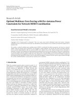
sented in Section 3.1.InFigure 1, we provide the simulated
signals, the CISA signal, affine functions A
i
, and shape fluc-
tuation functions n
i
. T he jitter variation is generated accord-
ing to β
i
= 0.1(i − (N − 1)/2) and the scale variation is given

by α
i
= 0.03(i − (N − 1)/2) + 1.
We estimate the CISA model parameters and functions
from the simulated signals by applying the procedure de-
fined in Section 2.2 after the integration and inversion op-
erations to obtain the X
−1
i
= z
i
. The convergence criterion is
fixed to Δ
˘
AISE
= 10
−5
.TheM values of y are equally sam-
pled in the interval [0.005, 0.995]. To apply the constraint of
(16), we use the two points [y
2
, y
M−1
] corresponding, re-
spectively, to the beginning and the end of the X
−1
i
= z
i
signals. The algorithm converges after 8 iterations giving

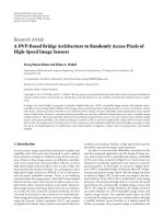
the results presented in Figure 2. We observe good estima-
tion of the CISA model with a final registration cost equal
to
˘
AISE
= 3.22 × 10
−7
. We also compute the RMS error
9876543210
Time
0
0.05
0.1
0.15
0.2
0.25
0.3
0.35
0.4
0.45
0.5
Amplitude
(a) Simulated signals (dashed curves), CISA signal (solid
curve), and the mean (thick curve)
9876543210
Time
0
1
2
3

4
5
6
7
8
9
Time
(b) The affine time functions A
i
9876543210
Time
0.2
0.15
0.1
0.05
0
0.05
0.1
0.15
0.2
Time
(c) The simulated shape fluctuation functions n
i
Figure 1: Simulation of signals using the CISA model.
between the CISA signal and its estimate and the ISA sig-
nal in
F
−1
,respectively,ase
RMS,μ

= 3.2 × 10
−4
and e
RMS,ISA
=
5.77 × 10
−2
. In addition, we calculated the nor malized RMS
6 EURASIP Journal on Advances in Signal Processing
error for the time parameter estimation computed as fol-
lows: e
RMS,α
i
=

(1/N)

N
i=1
(α
i
− α
i
)
2
/α
2
i
= 8.59 × 10
−4

and
e
RMS,

β
i
=

(1/N)

N
i=1
(

β
i
− β
i
)
2
/β
2
i
= 2.27 × 10
−2
.Wecan
observe in Figure 2 the difference between the ISA and CISA
signals. Although there are differences between the CISA and
ISA methods, the ISA remains a good choice for the initial-
ization procedure, and appears heuristically to place us close

to the minimum of the cost function.
Moreover, the difference between signal reference shapes
obtained using CISA and ISA methods can be explained the-
oretically. The expression for the ISA signal in
F
−1
is given by
[2]

X
−1
=
1
N
N

i=1
X
−1
i
. (24)
If we replace X
−1
i
by its expression in function of the CISA
signal, we obtain

X
−1
=

1
N
N

i=1

A
−1
i
◦ ω
i

◦

S
−1
. (25)
We replace also A
−1
i
and ω
i
by their expression and apply the
conditions 1/N

N
i
=1
β
i

/α
i
= 0and1/N

N
i
=1
1/α
i
= 1tofi-
nally obtain

X
−1
(y) =

S
−1
(y)+
1
N
N

i=1

n
i


S

−1
(y)

α
i

, y ∈ [0, 1].
(26)
From the equation, we explain the difference between ISA
and CISA signals by the bias introduced by the last term of
(26). In fact, the shape fluctuation functions are weighted by
the scale parameters. Two important remarks can be made in
relation to this point. First, if there is no shape fluctuation
among signals, ISA and CISA signals are superimposed. Sec-
ond, if there is only a jitter fluctuation, the two signals are
also superimposed. Otherwise, the two signals are different
and the CISA signal is the one that really averages the shapes
on an average time support without additional time fluctua-
tion contamination.
2.4. Shape clustering using CISA
Shape clustering provides a classification of signals based on
their shape. In order to provide a useful classification, we
need first to define the concept of shape equality. According
to [15], the signals x and y are said to be “equal in shape” if
and only if
y(t)
= ax

(t − β)
α


+ b. (27)
Since the proposed method is based on signal area registra-
tion, we assume that b
= 0 for all signals or in other words,
the offset term is removed before CISA calculation. Further-
more, to describe the shape statistics of a sample of signals
while respecting the shape equality condition, one needs to
define [3]:
(i) a distance d between signals which is in fact a distance
between the signal shapes. A natural consequence of
this is that if we take two signals x and y, then d(x, y)
=
0 ⇔ x and y are “the same shape.” Thus, this shape
distance is invariant to affine transforms,
(ii) a sample mean that is intrinsically invariant in shape
to the affine transforms described in (27), and hence
a mean which provides a realistic average shape signal
[3]. In addition, this mean shape signal must have the
property of being a “shape gravity center” with respect
to the shape distance d. We can easily demonstrate that
the CISA signal coupled with the CISA distance has
such properties. In fact, if we define the CISA distance
between two signals x
1
and x
2
that belong to a sample
of N signals as
d

CISA

x
1
, x
2

=


1
0

A
1

X
−1
1
(y)

−
A
2

X
−1
2
(y)


2
dy,
(28)
then the CISA distance can be interpreted as the
L
2
[0, 1] norm in F
−1
between the two registered and
area-normalized signals. It can also be expressed as
d
CISA

x
1
, x
2

=


1
0

n
1


S
−1

(y)

−
n
2


S
−1
(y)

2
dy.
(29)
In this last expression, the CISA distance is expressed as a
function of the shape fluctuation referred to the CISA signal.
This quantity does represent a true shape distance, as demon-
strated by the following. Since the CISA sig nal is the mean of
the registered sig nals A
i
◦ X
−1
i
in F
−1
,wecanwrite

S
−1
= arg min

u∈R
N

i=1
d
2

u, A
i
◦ X
−1
i

=
1
N
N

i=1
A
i
◦ X
−1
i
. (30)
This last equation expresses the shape variance minimiza-
tion propert y of the CISA signal. Indeed, the CISA sig-
nal is a “shape gravit y center.” As shown above, both the
CISA signal and distance by definition are invariant to affine
transforms.

To perform shape clustering, we can use the well-known
k-means approach [16]. The method consists of separating
signals into classes (clusters) that maximize interclass vari-
ance and minimize intraclass var iance. It can alternatively
be expressed as a global minimization problem in which the
quantity to minimize is the sum of distances to the nearest
neighbor. Classically, the method employs the conventional
mean and the L
2
distance in R as class center and clustering
S. Boudaoud et al. 7
10.90.80.70.60.50.40.30.20.10
Amplitude
0
1
2
3
4
5
6
7
8
Time
(a) The X
−1
i
= z
i
signals (dashed line) and the regis-
tered

ˆ
g
i
ones in F
−1
(solid line)
1086420
Signals
0.5
0.4
0.3
0.2
0.1
0
0.1
0.2
0.3
0.4
0.5
Estimated jitter (time)
1086420
Signals
0.85
0.9
0.95
1
1.05
1.1
1.15
1.2

Estimated scale
(b) The estimated jitter and scale parameters
876543210
Time
0
0.2
0.4
0.6
0.8
1
Amplitude
CISA
ISA
ECISA
(c) The ISA, the theoretical CISA, and the estimated CISA
signals
6.565.554.543.532.521.5
Time
0.2
0.15
0.1
0.05
0
0.05
0.1
0.15
0.2
Time
(d) The estimated shape fluctuation functions
ˆ

n
i
876543210
Time
0
0.2
0.4
0.6
0.8
1
Normalized amplitude
(e) The registered
ˇ
x
i
signals
Figure 2: Estimation of the CISA model from the simulated data.
8 EURASIP Journal on Advances in Signal Processing
6.565.554.543.532.521.5
Time
0
20
40
60
80
100
120
140
160
180

200
Normalized amplitude
Figure 3: The final CISA class centers from the simulated data.
distance, respectively. In the presence of time fluctuations,
these tools give bad clustering performances. To deal with the
time fluctuations, we propose to use the k-means algorithm
to cluster signal shapes in
F
−1
, by using the CISA signal and
distance as class center and distance, respectively. This has al-
ready been done for a biomedical application using the ISA
approach [6, 7] using a similarity criterion rather than a dis-
tance. However, as mentioned previously, the ISA center does
not necessarily possess a gravity center property.
To illustrate the utility of the CISA method, we first pro-
pose to apply it for clustering the signals of the preceding
simulation example into two classes. Firstly, all the signals
are registered to eliminate affine fluctuation. Then, the k-
means algorithm is launched with random class center ini-
tialization chosen from among the
ˇ
x
i
signals. The CISA sig-
nal is then computed until convergence for each class and
a discrete version of CISA distance is used. The procedure
is repeated L times. The final clustering solution is selected
based on class separation criterion maximization and solu-
tion redundancy. The separation criteri on represents the ra-

tio between the final interclass center distance and the sum of
both intraclass distance standard deviations. A ratio greater
than 1 indicates good class separation. For our example, the
10 signals are well classified and the final class centers can be
seen in Figure 3. The clustering criterion obtained is equal
to R
= 5.51, indicating a high shape separation between the
two classes. This validates that the CISA methodology can be
used to provide accurate classification of signals based solely
on shape differences. Indeed, the use of this parameter re-
spects the unsupervised nature of the classification (no use
of a priori information). Other criteria should be designed
to measure classification performances of a particular appli-
cation. Practically, affiliation of the obtained classes to the
healthy and pathological ones should be done using some
a priori information or specific characteristics of the class
(shape dispersion). In our case study, we will assume that the
classification done by the expert is perfect. So, the class af-
filiation will be done according to signals which lie mostly
within their correct class.
3. OBSTRUCTIVE SLEEP APNEA DETECTION
As discussed in the introduction, obstructive sleep apnea
(OSA) is a common sleep disorder with many physiological
consequences, such as increased risk of cardiovascular dis-
ease, hypertension, and daytime sleepiness. Previously tech-
niques have been developed to recognize periods of sleep
apnea from the ECG by using RR interval variability, and
an ECG-derived respiratory signal. However, no previous
approaches have considered morphological changes of the
ECG due to OSA. Such changes, especially for the P-wave

or T-wave, could have an underlying physiological plausibil-
ity as ischemia due to oxygen desaturation could alter the
electrical activation of the atria and ventricles [17, 18]. In
a recent study, we showed a strong correlation between P-
wave shape changes and the occurrence of OSA events. How-
ever, this initial approach used an improvement of the ISA
method (with consequent incomplete theoretical foundation
as a shape clustering technique) and presented analysis on a
small subset of signals. In this current work, we use the CISA
methodology on a larger set of signals to provide a robust
classification of ECG segments.
3.1. P-wave shape clustering
In this section, we discuss results on the use of the CISA sig-
nal and distance coupled with a k-means algorithm for de-
veloping an unsupervised shape classifier. The method is ap-
plied to perform a clustering [8] on P-wave shapes extracted
from 163 ECG segments sampled at 128 Hz. These segments
areeach2minutesinlengthandwereacquiredfrom7sub-
jects who suffer from OSA. For these segments, 95 are con-
sidered as normal and 68 are centered on a discrete episode
of OSA of 10 second duration or longer. The ECG segments
were extracted from complete polysomnogram recordings
carried out at St. Vincent’s University Hospital, D ublin, using
the Jaeger-Toennies polysomnogram system.
The epoch labeling was obtained from the polysomno-
gram analysis by an expert. For each segment, the P-waves
were segmented according to the QRS complex, baseline cor-
rected after upsampling (by a factor of five) and spline fil-
tering. The artifacts were also removed by amplitude thresh-
old selection as follows: for each segment, a shape homo-

geneous P-wave set was detected by shape analysis. In fact,
the CISA procedure was performed for one iteration for each
segment. For this purpose, discrete versions of both the CISA
signal and distance expressions were used. After that, sig-
nals within one standard deviation of CISA distance from the
CISA mean were selec ted. These signals were averaged to pro-
vide us with the overall segment shape prototype. This proce-
dure avoids shape contamination of the segment representa-
tive signal by noisy signals (e.g., the P-wave corresponding to
a premature atrial contraction or normal P-waves inside an
apneic segment). For each subject, the segment prototypes
were then registered following the CISA procedure after ade-
quate windowing procedure. The convergence criterion was
fixed to Δ
˘
AISE
= 10
−5
and the inverse distribution inter-
val was set to y
= [0.02, 0.96]. Then, a two-class (normal,
apnea) clustering was done on the segment prototypes for
S. Boudaoud et al. 9
Table 1: CISA shape clustering results.
Subject No. of normal segments No. of apnea segments Sens. (%) Spec. (%) R
115 1191931.95
2 10 8 87 80 1.94
315 1070730.74
4 10 10 60 100 2.83
515 1090801.34

615 1080861.35
7 15 9 88 73 1.31
Average — — 80.9 83.6 —
L = 15 trials following the procedure described in Section 2.3
for each subjec ts So ideally for a single subject represented
(e.g.) with ten “normal” segments and twelve “apnea” seg-
ments we hope to achieve a clustering into two classes which
have 10 and 12 members, respectively, each belonging cor-
rectly to the classes “normal” and “apnea.” For the 7 sub-
jects studied in this paper, the results are shown in Tabl e 1.
For each subject, the number of normal and apneic segments
and the class separation criterion R value are indicated. These
segment numbers correspond to the classification done by
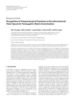
the expert and assumed to be perfect. In Figure 4, we show
the original and registered P-wave prototypes using the es-
timated affine parameters for the recordings from Subject 2.
We can also observe the final CISA class centers obtained by
the approach. We can observe a significant shape difference
between the two signals. For most subjects, the class separ a-
tion is good according to the R value. As can be observed,
the proposed method reached an overall sensitiv ity of 80.9 %
and specificity of 83.6 % and maximum sensitivity of 91 %
and maximum specificity of 93 %. This result confirms the
earlier results obtained on a smaller database in [8], the exis-
tence of a strong correlation b etween P-wave shape variation
and the occurrence of OSA.
3.2. Relation between time variations of
the P-wave and apnea
In addition to shape fluctuation estimation, the CISA
method also simultaneously permits an estimation of the

affine time parameters (scale and jitter) used in the realign-
ment procedure (see Section 2.2). It is plausible that changes
in these parameters can be linked to OSA occurrence and
also be used to recognize apnea episodes. Both scale and jitter
were estimated from the segment prototypes of each subject
following the estimation procedure described in Section 2.2.
We then tried to find some correlation (by true classification)
between the variation of these parameters and the labeling
of the corresponding segments (normal or apneic) for each
subject done by the expert. For two subjects, the scale param-
eter variation dominated and showed a clear increase in the
P-wave duration during OSA. A scale threshold α
thr
= 1was
used which maximizes the classification performance (based
on maximizing of the sum of specificity and sensitivity) for
the two classes (normal and apnea) of the concerned seg-
ment prototypes based solely on the scale estimated parame-
ter. This value corresponds to the reference scale of the CISA
signal. Indeed, scale and jitter parameters are relative values
referring to the CISA signal. The classification was based on
a simple threshold decision rule. If the scale parameter α
i
is
greater than one (signal dilation), this means that the corre-
sponding segment is apneic; otherwise it is classified as nor-
mal. The results for this analysis are shown in Ta ble 2 .Inad-
dition, for two other subjects, the effects of apnea were to
provide combined jitter and scale variation. For the classifi-
cation task, therefore, we used a parameter that mixes both

scale and jitter γ
i
= β
i
/α
i
. For these two subjects, we tried to
find a threshold γ
thr
that maximizes the classification perfor-
mance. For a subject, if the parameter γ
i
is greater than γ
thr
,
the signal is considered as apneic, otherwise it is normal. The
results obtained are shown on Ta ble 3 . In the three remain-
ing subjects, time parameters variation was not significantly
correlated to OSA occurrence. We conclude, therefore, that
apnea episodes can affect both the time duration and timing
of the P-wave (PR interval) but in a subject-specific fashion.
4. CONCLUSIONS
In this paper, we have presented a novel method, corrected
integral shape averaging (CISA), for signal realignment and
shape fluctuation estimation. The method is based on a sig-
nal model that includes both shape and time support varia-
tion of the signal distribution functions. The CISA approach
provides us with a new mean shape signal, the CISA signal,
that possesses interesting mathematical properties for signal
shape characterization. In fact, coupled to the CISA distance,

the CISA signal minimizes shape fluctuation variance over a
set of signals to be averaged. In addition, it is not contami-
nated by affine time fluctuations as for a related method us-
ing integral shape averaging. These useful properties make
the CISA signal a good candidate for shape clustering appli-
cations. The CISA model contains a number of unknown pa-
rameters relating to time and shape variation, and we have
described an iterative estimation procedure for obtaining the
values of these parameters. The performance of the CISA
procedure is illustrated using a controlled numerical simu-
lation, a nd it can be shown that it clearly classified synthetic
signals into their correct classes despite the presence of time
fluctuations. The method was then applied to evaluate the
benefits of using P-wave shape to recognize obstructive sleep
apnea in ECG recordings. Using the k-means algorithm, the
10 EURASIP Journal on Advances in Signal Processing
6050403020100
Time (ms)
0
1
2
Amplitude (mV)
(a) The normal (–) and the apneic P-waves (– –) (ac-
cording to expert labeling) before realignment
6050403020100
Time (ms)
0
1
2
Amplitude (mV)

(b) The normal (–) and the apneic P-waves (– –) after
realignment
5045403530252015
Time (ms)
0
0.5
1
1.5
2
2.5
3
Amplitude (arbitrary units)
(c) The final CISA class centers (normal –, apneic – –)
Figure 4: Results of CISA averaging technique applied to the P-wave
segments measured in Subject 2.
method p erformed a clustering operation on a database of
163 signals. The classification results confirmed, in a more
rigorous fashion, the important correlation linking P-wave
shape and OSA episodes occurrence described in a previous
work. A true classification procedure (based on the knowl-
edge of the perfect classification) using the time parameters
(scale and jitter) estimated by the CISA method was also pro-
posed and applied on some subjects. The obtained results
showed also a time alteration of the P-wave induced by OSA
occurrence in a patient-specific manner.
A limitation of the study was the relatively low sam-
pling rate for ECG, and we expect that future studies using
ECG measurements with higher sampling rate would im-
prove the shape analysis performances. Since the objective
of the paper was the rigorous confirmation of the correlation

between shap e changes and apnea occurrence, the following
step would be the design of an apnea “detector” using shape
information. This dev ice should use the P-wave shape varia-
tion also combined with the existing RR interval variability
and EDR techniques to improve overall classification perfor-
mance. However, the proposed CISA approach could also be
used to analyze other bioelectrical signals such as other ECG
components or brain-evoked potentials.
In conclusion, the CISA method and its application high-
light the potential of signal shape analysis by time-warping
estimation for signal description. In fact, both minimizing
the signal parametrization and functional modeling permit
a direct access to signal shape information and implicitly
to generation process properties. In biomedical applications,
dealing with shape and time warping may assist in providing
plausible physiological models for signal generation.
APPENDIX
CISA MODEL IDENTIFIABILITY
In this section, we prove the identifiability of the proposed
CISA model. For this purpose, we suppose that there exists
two different solutions μ and μ

, that is, z
i
signals are linked to
μ and μ

, respectively, by the following CISA model equations
without noise in
F

−1
:
μ(y)
= α
i
z
i
(y)+β
i
+ w
i
(y), ∀i = 1:N, y ∈ [0, 1],
μ

(y) = α

i
z
i
(y)+β

i
+ w

i
(y), ∀i = 1:N, y ∈ [0, 1].
(A.1)
If we replace z
i
expression from the first equation in the sec-

ond one
μ

(y) =
α

i
α
i
μ(y)+

β

i
−
β
i
α

i
α
i

+

w

i
(y) −
α


i
α
i
w
i
(y)

.
(A.2)
We rewrite the equation to the form
μ

(y) = A
i
μ(y)+B
i
+ g
i
(y), ∀i = 1:N. (A.3)
The first term of the equation being independent of i,wecan
write for i
= k and i = l
μ

(y) = A
k
μ(y)+B
k
+ g

k
(y), y ∈ [0, 1]
μ

(y) = A
l
μ(y)+B
l
+ g
l
(y), y ∈ [0, 1].
(A.4)
S. Boudaoud et al. 11
Table 2: Classification based on scale parameter.
Subject No. of normal segments No. of apnea segments Sens. (%) Spec. (%) α
thr
115 1182731
2 10 8 87 80 1
Average — — 84.5 76.5 —
Table 3: Classification based on both jitter and scale parameters.
Subject No. of normal seg ments No. of apnea segments Sens. (%) Spec. (%) γ
thr
(ms)
410 1080800
7 15 9 88 73 0.8
Average — — 84 76.5 —
We subst ract the second equation from the first

A
k

− A
l

μ(y)+

B
k
− B
l

,
+

g
k
(y) − g
l
(y)

=
0, ∀y ∈ [0, 1].
(A.5)
Then we apply the conditions g
i
(0) = 0andg
i
(1) = 0 (from
conditions on w
i
and w


i
) for the two values y = 0andy = 1
where μ(0)
= t
inf
and μ(1) = t
sup
and obtain

A
k
− A
l

t
inf
+

B
k
− B
l

= 0

A
k
− A
l


t
sup
+

B
k
− B
l

=
0.
(A.6)
From these two equations, we can deduce that A
k
= A
l
= A
and B
k
= B
l
= B since t
inf
= t
sup
. In addition, we can add
after replacing these last parameters in (A.5) that g
k
= g

l
= g
for all y. Finally, we rewrite (A.3) in the form
μ

(y) = Aμ(y)+B + g(y), (A.7)
where A
= α

i
/α
i
, B = β

i
− β
i
α

i
/α
i
,andg(y) = w

i
(y) −
(α

i
/α

i
)w
i
(y) are quantities independent of indexed i.
Computing the mean of A/α

i
and applying the condi-
tions on the scale parameters in (5)giveA
= (1/N

N
i
=1
1/α
i
)/
(1/N

N
i=1
1/α

i
) = 1. This means that α
i
= α

i
for all i.

Computing the mean of B/α

i
and applying the con-
ditions on both scale and jitter parameters in (5)give
B/N

N
i
=1
1/α

i
= [1/N

N
i
=1
β

i
/α

i
−1/N

N
i
=1
β

i
/α
i
] = 0. Since
A
= 1andB = 0, we obtain β
i
= β

i
from the expression of B
for all i.
Computing the mean of g and a pplying the conditions
on n
i
in (5) (which are the same for w
i
and w

i
)giveg(y) =
[1/N

N
i
=1
w

i
(y) − A/N


N
i
=1
w
i
(y)] = 0forally ∈ [0, 1].
This means that w
i
(y) = w

i
(y)forally ∈ [0, 1] and i.
Finally, if we replace A, B,andg by their value, respec-
tively, we obtain μ(y)
= μ

(y)forally ∈ [0, 1] which com-
pletes the proof. In fact, the CISA model is identifiable.
ACKNOWLEDGMENT
This work was suppor ted by a doctoral grant referenced as
394114L from Provence, Alpes, C
ˆ
ote d’Azur (PACA) region,
France, and MXM Laboratories, Vallauris, France.
REFERENCES
[1]J.O.RamsayandB.W.Silverman,Functional D ata Analysis,
Springer Series in Statistics, Springer, New York, NY, USA,
1997.
[2] S. Boudaoud, H. Rix, and O. Meste, “Integral shape averaging

and structural average estimation: a comparative study,” IEEE
Transactions on Signal Processing, vol. 53, no. 10, pp. 3644–
3650, 2005.
[3] S. Boudaoud, H. Rix, and O. Meste, “Providing sample shape
statistics with FCA and ISA approaches,” in Proceedings of the
13th Workshop on Statistical Signal Processing (SSP ’05),pp.
443–448, Bordeaux, France, July 2005.
[4] H. Rix, O. Meste, and W. Muhammad, “Averaging signals with
random time shift and time scale fluctuations,” Methods of In-
formation in Medicine, vol. 43, no. 1, pp. 13–16, 2004.
[5] H.RixandJ.P.Maleng
´
e, “detecting small variations in shape,”
IEEE Transactions on Systems, Man, and Cybernetics, vol. 10,
no. 1, pp. 90–96, 1980.
[6] H. Rix, S. Boudaoud, and O. Meste, “Clustering signal shapes:
applications to P-waves in ECG,” in Proceedings of the 2nd
European Medical and Biological Engineering Conference (EM-
BEC ’02), pp. 364–365, Vienna, Austria, December 2002.
[7] S. Boudaoud, H. Rix, J. J. Blanc, J. C. Cornily, and O. Meste,
“Integrated shape averaging of the P-wave applied to AF risk
detection,” in Proceedings of the 30th Annual International
Conference of Computers in Cardiology, vol. 30, pp. 125–128,
Thessaloniki, Greece, September 2003.
[8] S. Boudaoud, C. Heneghan, H. Rix, O. Meste, and C. O’Brien,
“P-wave shape changes observed in the surface electrocardio-
gram of subjects with obstructive sleep apnoea,” in Proceedings
of the 32nd Annual International Conference on Computers in
Cardiology, pp. 359–362, Lyon, France, September 2005.
[9] T. Young, L. Evans, L. Finn, and M. Palta, “Estimation of the

clinically diagnosed proportion of sleep apnea syndrome in
12 EURASIP Journal on Advances in Signal Processing
middle-agedmenandwomen,”Sleep, vol. 20, no. 9, pp. 705–
706, 1997.
[10] A. S. M. Shamsuzzaman, B. J. Gersh, and V. K. Somers, “Ob-
structive sleep apnea: implications for cardiac and vascular
disease,” Journal of the American Medical Association, vol. 290,
no. 14, pp. 1906–1914, 2003.
[11] R. S. T. Leung and T. D. Bradley, “Sleep apnea and cardiovascu-
lar disease,” American Journal of Respiratory and Critical Care
Medicine, vol. 164, no. 12, pp. 2147–2165, 2001.
[12] T. Penzel, J. McNames, P. de Chazal, B. Raymond, A. Mur-
ray, and G. Moody, “Systematic comparison of different al-
gorithms for apnoea detection based on electrocardiogram
recordings,” Medical and Biological Engineering and Comput-
ing, vol. 40, no. 4, pp. 402–407, 2002.
[13] J. O. Ramsay and X. Li, “Curve registration,” Journal of the
Royal Statistical Society. Series B, vol. 60, no. 2, pp. 351–363,
1998.
[14] D. Ger vini and T. Gasser, “Self-modelling warping functions,”
Journal of the Royal Statistical Society. Series B, vol. 66, no. 4,
pp. 959–971, 2004.
[15] W. H. Lawton, E. A. Sylvestre, and M. S. Maggio, “Self mod-
eling non linear regression,” Technometrics, vol. 14, no. 3, pp.
513–532, 1972.
[16] A. K. Jain, R. P. W. Duin, and J. Mao, “Statistical pattern recog-
nition: a review,” IEEE Transactions on Pattern Analysis and
Machine Intelligence, vol. 22, no. 1, pp. 4–37, 2000.
[17] J. Carlson, R. Johansson, and S. B. Olsson, “Classification of
electrocardiographic P-wave morphology,” IEEE Transactions

on Biomedical Engineering, vol. 48, no. 4, pp. 401–405, 2001.
[18] P. E. Dilaveris and J. E. Gialafos, “Future concepts in P-
wave morphological analyses,” Cardiac Electrophysiology Re-
view, vol. 6, no. 3, pp. 221–224, 2002.
S. Boudaoud was born in B
´
eja
¨
ıa, Alge-
ria, in May 1975. He received the Engi-
neer grade in electrical and electronic en-
gineering from the University A. Mirra of
B
´
eja
¨
ıa, Algeria, in 1998, the M.S. degree in
electrical and electronic engineering from
the University F. Abbas of S
´
etif, Algeria, in
2001, and the M.S. degree in signal pro-
cessing and communication from the Uni-
versity of Nice-Sophia Antipolis, France, in
2002. He completed the Ph.D. degree in automatic, signal, and im-
age processing in 2006 at the University of Nice-Sophia Antipolis.
Currently, he is a Temporary Assistant Professor at the BIOMED
Group, Laboratory of Informatic, Signals & Systems of Sophia An-
tipolis, France. His research interests are in signal processing and
modeling applied to biomedical fields.

H. Rix received the M.S. degrees in as-
trophysics (1968) and applied mathemat-
ics (1969), the “Doctorat de Sp
´
ecialit
´
e” de-
gree in astrophysics (1970), and a “Doctorat
d’Etat” in sciences (1980) from the Univer-
sity of Nice, France. He has been a Profes-
sor with the University of Nice since 1987.
His research field is signal processing mainly
applied to biomedical signals. At the Labo-
ratory of Informatics, Signals & Systems of
Sophia Antipolis, he heads the BIOMED Group.
O. Meste received the M.S. degree in au-
tomatic and signal processing and the
Ph.D. degree in scientific engineering from
the University of Nice-Sophia Antipolis,
France, in 1989 and 1992, respectively. He
is currently working as a Professor at the
University of Nice-Sophia Antipolis and as a
Researcher at the Biomed Project of the I3S
Laboratory. His research interests are in dig-
ital processing, time-frequency representa-
tions, and modeling to biological signals and systems.
C. Heneghan was born in Dublin, Ireland,
in 1968 and received the B.E. degree in elec-
tronic engineering from University College
Dublin, in 1990 and the Ph.D. degree in

electrical engineering from Columbia Uni-
versity, New York, NY, in 1995. He is cur-
rently an Associate Professor in the School
of Electrical, Electronic, and Mechanical
Engineering at University College Dublin,
as well as serving as the Chief Scientific Offi-
cer of BiancaMed Ltd., an ambient health and wellness monitoring
company. He has previously been the Director of Tele-Informatics
at the New York Eye and Ear Infirmary, a Visiting Associate Profes-
sor at Stanford University’s Information Systems Laboratory, and
a Visiting Researcher at the Laboratoire Informatique Signaux et
Systemes de Sophia Antipolis (I3S). He is a Member of the IEEE
Engineering in Medicine and Biology Society, the Signal Process-
ing Society, and the Communications Society. He is a reviewer for
several journals including the IEEE Transactions on Biomedical En-
gineering and IEEE Transactions on Signal Processing. His research
interests include signal processing for biomedical applications and
signal processing for communications.
C. O’Brien was born in Dublin, Ireland, in
1978 and received the B.E. degree in elec-
tronic engineering from University College
Dublin in 2000. She completed the Ph.D.
degree in electronic engineering in Univer-
sity College Dublin in 2006. Her thesis topic
was based on signal processing of a reduced
number of biomedical recordings for auto-
mated detection of events during sleep such
as sleep apnea or sleep staging. The signal
processing involved is based on pattern recognition and signal sep-
aration. She is a Member of Engineers Ireland.