Báo cáo hóa học: " Research Article Duct Modeling Using the Generalized RBF Neural Network for Active Cancellation of Variable Frequency Narrow Band Noise" pot

Hindawi Publishing Corporation
EURASIP Journal on Advances in Signal Processing
Volume 2007, Article ID 41679, 7 pages
doi:10.1155/2007/41679
Research Article
Duct Modeling Using the Generalized
RBF Neural Network for Active Cancellation of
Variable Frequency Narrow Band Noise
Hadi Sadoghi Yazdi,
1
Javad Haddadnia,
1
and Mojtaba Lotfizad
2
1
Engineer ing Department, Tarbiat Moallem University of Sabzevar, P.O. Box 397, Sabzevar, Iran
2
Department of Electrical Engineering, Tarbiat Modarres University, P.O. Box 14115-143, Tehran, Iran
Received 27 April 2005; Revised 1 February 2006; Accepted 30 April 2006
Recommended by Shoji Makino
We have shown that duct modeling using the generalized RBF neural network (DM
RBF), which has the capability of modeling
the nonlinear behavior, can suppress a variable-frequency narrow band noise of a duct more efficiently than an FX-LMS algorithm.
In our method (DM
RBF), at first the duct is identified using a generalized RBF network, after that N stageoftimedelayofthe
input signal to the N generalized RBF network is applied, then a linear combiner at their outputs makes an online identification
of the nonlinear system. The weights of linear combiner are updated by the normalized LMS algorithm. We have showed that
the proposed method is more than three times faster in comparison with the FX-LMS algorithm with 30% lower error. Also the
DM
RBF method will converge in changing the input frequency, while it makes the FX-LMS cause divergence.
Copyright © 2007 Hindawi Publishing Corporation. All rights reserved.

1. INTRODUCTION
In the recent years, acoustic noise canceling by active meth-
ods, due to its numerous applications, has been in the fo-
cus of interest of many researches. Contrary to the passive
method, it is possible using the active method to suppress or
reduce the noise in a small space particularly in low frequen-
cies (below 500 Hz) [1, 2]. Active noise control was intro-
duced for the first time by Paul Lveg in 1936 for suppressing
the noise in a duct [3]. In the active control method by pro-
ducing a sound with the same amplitude but with opposite
phase, the noise is removed. For this purpose, the amplitude
and phase of a noise must be detected and inverted. The de-
veloped system must have the adaptive noise control capabil-
ity [3]. In usual manner, an FIR filter is used in ANC whose
weights are updated by a linear algorithm [4, 5]. Using the
linear algorithm of LMS is not possible due to the nonlinear
environment of the duct and the appearing of the secondary
path transfer function H(z). Hence, the FX-LMS algorithm
is presented in which the filtered input noise x

(n) is used as
an input to the algorithm [6, 7]. The notable points in ANC
areasfollows.
(i) The duct length and the distance between the system
elements are such that the system becomes causal [8].
(ii) Regarding the speaker response, no decrease will be
obtained in frequencies below 200 Hz [2]. Also passive
techniques for reducing the noise in frequencies below
500 Hz have not been successful [1, 2]. Therefore, the
ANC systems are used in the range of 200 to 500 Hz

and above 500 Hz.
The existence of nonlinear effects in ANC complicates the use
of the linear algorithm FX-LMS and similar algorithms. Di-
vergence or slow convergence is among these difficulties. For
this purpose, identification systems with a nonlinear struc-
ture are used where a neural network is among these solu-
tions [9–11]. The radial basis function (RBF) networks are
used in processing temporal signals for radar [12], in the
predictor filter in position estimation from present and past
samples [13], and in adaptive prediction and control [14, 15].
Buffering data, feedback from the output of the system, and
state machines are used in modeling temporal signals. In
time delay RBF neural networks, also, by buffering data [16],
and using the feedback from the output in the recurrent RBF
(RRBF) [17], this work is accomplished.
In the present work a new structure with the generalized
RBF neural network is presented whereby a linear combi-
nation of the outputs of N neural networks causes a time
varying nonlinear system being modeled. Samples x(n)to
2 EURASIP Journal on Advances in Signal Processing
c(z)
W(z)
LMS
H(z)
x
(n)
x(n)
y(n)
y
(n)

e(n)
L
ANC controller
Input microphone
Primary noise
Noise source
Canceling speaker
Error
microphone
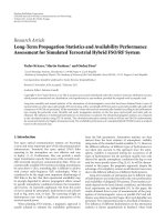
Figure 1: Using the FX-LMS algorithm in a single channel ANC
system.
x( n − N +1)arefedtoN generalized RBF neural networks
and then the linear combination of their outputs is used for
canceling the acoustic noise inside a duct. For precise sim-
ulation of the proposed algorithm and comparison to the
conventional FX-LMS method, the t ransfer function of the
primary path (the duct transfer function) and the secondary
path must be available, which for this purpose, the informa-
tiongivenin[18] which is obtained practically is utilized.
Section 2 of this paper concerns the investigation of the
active noise control in a duct and the FX-LMS algorithm.
Section 3 contains a short review of the RBF and general-
ized RBF neural networks. In Section 4, the proposed system
and its application in ANC are presented and in Section 5 the
conclusions are presented.
2. PRINCIPLE OF ACTIVE NOISE CONTROL
IN A DUCT
If we assume the noise propagates in a one-dimensional
form, then it is possible to use a single channel ANC for
noise cancellation. For simulation and implementation of

this system, a narrow duct is used as in Figure 1. According
to Figure 1, the pr imary noise before reaching to the speaker
is picked up by the input microphone. The system uses the
input signal for generating the noise canceling signal y(n).
The generated sound by the speaker gives rise to a reduc-
tion in the primary noise. The error microphone measures
the remaining signal e(n) which can be minimized using an
adaptive filter which is used for identifying the duct’s transfer
function. Because of using the input and error microphones,
we must consider some functions which are known as the
secondary path effects. In such a system, usually for cancel-
ing the noise, the FX-LMS algorithm, Figure 1,and(1)are
considered [1, 19–21]. The vector x

(n)isafilteredcopyof
the vector x(n).
W
n+1
= W
n
− μe
n
X

n
,(1)
where e
n
is the residual signal and W
n

= [w
n
(1), w
n
(2), ,
w
n
(M)]
T
is the weight vector of the estimator of length M.
x
m
x
m 1
x
1
.
.
.
Input layer
Hidden layer
ϕ
ϕ
ϕ
.
.
.
ϕ
w
m

w
1
1
w
0

F
Output layer
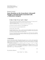
Figure 2: Structure of an RBF network.
In Figure 1, the c(z) is an estimation of H(z) which can be
obtained by some offline techniques [22]. The considerable
points in the execution the FX-LMS are the following.
(i) Canceling the broadband noise needs a filter of high
order which increases the duct length [22].
(ii) In order to choose the proper stepsize, we need the
knowledge of statistical properties of the input data
[23, 24].
(iii) To ensure the convergence, the stepsize is chosen small;
hence the convergence speed will be low and the per-
formance will be weak.
(iv) For executing the above algorithm, we need to estimate
the secondary path.
(v) This algorithm is only applicable to a linear controller
and is not either suitable for nonlinear controllers or
it is slow. For modeling the nonlinear behavior of this
system, neural networks can be employed.
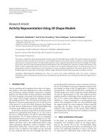
3. THE RBF NEURAL NETWORKS
The RBF networks usually have three layers as shown in
Figure 2. The first layer comprises the input nodes, the sec-
ond layer, which is a hidden layer, includes a nonlinear trans-

formation, and the third layer includes the output layer. The
output in terms of the input is given by
F
j
(x) =
r

i=1
w
ij
ϕ
i



x − c
i


, δ
i

,(2)
where F
j
(x) is the response of the jth neuron in the input
feature vector x and W
ij
is the value of the interconnection
weight between the ith neuron in the RBF layer and the jth

neuron in the output layer.
x − c
i
 represents the Euclidean
distance and ϕ
i
is the stimulation function of the ith neurons
in the RBF layer which is also called the kernel. The kernel
can be chosen as a simple norm or a Gaussian function or
any other suitable function [25]. In practice it is chosen as a
Gaussian function which in this case F is a Gaussian mixture
function and each neuron in the RBF layer is identified by the
two parameters center c
i
and width δ
i
.
Hadi Sadoghi Yazdi et al. 3
x(n)
x
1
x(n 1)
x
1
x(n 2)
x
1
x(n N)
GRBF GRBF
GRBF

GRBF
f
0
α
0
f
1
α
1
f
2
α
2
f
N
α
N
LMS
+
+
+
+

F
+

d(n)
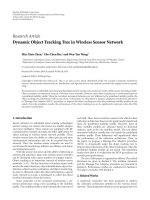
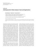
Figure 3: Structure of the proposed method.
3.1. The generalized RBF neural network
In this paper, the generalized neural network is used for mod-

eling the duct. In this type of RBF, the ϕ
i
(x)functioniscom-
puted as [25]
ϕ
i
(x) = G



x − c
i



=
exp

−
1
2

x − c
i

T

−1

x − c

i


,
(3)
where

is the covariance matrix of the input data and c
i
are
the centers of the Gaussian functions. The optimum weight
vector is obtained as
W
=

G
T
G

−1
G
T
d,(4)
where d is the desired value and G is the Green func-
tion which for k inputs x
1
to x
k
and G aussian centers c =
[c

1
, , c
m
], its Green Function is as follows:
G
=
⎡
⎢
⎢
⎢
⎢
⎢
⎢
⎣
G

x
1
, c
1

G

x
1
, c
2

··· G


x
1
, c
m

G

x
2
, c
1

G

x
2
, c
2

···
G

x
2
, c
m

.
.
.

.
.
.
.
.
.
G

x
k
, c
1

G

x
k
, c
2

···
G

x
k
, c
m

⎤
⎥

⎥
⎥
⎥
⎥
⎥
⎦
,(5)
where x
k
is the kth learning sample.
4. THE PROPOSED ALGORITHM
The time delay neural network presented in this paper in-
cludes N stages which are illustrated in Figure 3. At first, the
duct is identified by the generalized RBF, GRBF, and then the
results are combined by a linear adaptive filter such as LMS.
Because of changing space with GRBF, obtaining error will
be less than input space or the MSE at Φ-space is smaller
than the input space; so we expect LMS has had smaller er-
ror without converting space. This subject has been proved
in the appendix.
The relation between the output and the input is given in
F
=
N

j=0
α
j
· f
j


x( n − j)

,
F
=
N

j=0

α
j
m

i=1
w
i
G



x( n − j) − c
i




,
(6)
where N is the number of the delayed input signal samples

and m is the number of the used kernels in the generalized
RBF network. w
i
s are obtained from (4)andα
j
s are updated
with LMS algorithm according to
A
n+1
= A
n
− 2μ · Y
n
· e
n
,(7)
where A
n
= [α
n
(1), α
n
(2), , α
n
(N)]
T
, Y
n
= [ f
n

(1),
f
n
(2), , f
n
(N)]
T
,ande
n
is the system error which is ob-
tained from subtracting the system output, F from the de-
sired value of the signal, d
n
at instant n. In noise reduction
problem, and d
n
is the primary noise which reaches the exci-
tation speaker.
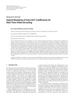
4.1. Applying the proposed algorithm in
active noise canceling
The present network is used to active noise cancel as in
Figure 4. At instant two points are interested in the proposed
system as
(a) deletion of secondary path estimation c(z),
(b) learning the transfer function of GRBF and the linear-
ity of active noise control system using this idea.
In the next subsections duct modeling and noise cancel-
lation are explained.
4.2. Duct system function identification
We begin first by identifying the duct with the GRBF and

the proposed system and then compare them. Equation (3)
is found by fuzzy k-means clustering. In this problem, 4
centers are used. Therefore, 4 Gaussian functions are ob-
tained. Equation (3) is also rewritten in the form of (8). The
4 EURASIP Journal on Advances in Signal Processing
x(n)
H(z)
y(n)
e(n)
L
Input
microphone
Primary noise
Noise source
Cancelling
speaker
Error
microphone
The proposed
algorithm
Figure 4: A str ucture for noise canceling in a duct by the proposed
method.
Gaussian kernels of the GRBF function are computed using
(9), (4.2).
ϕ
i
(x) = G




x − c
i



=
exp

−
1
2σ
i



x − c
i


2


,(8)
σ
i
=






k
1
m=1

x
m
− c
i

2
k
1
− 1
,(9)
x
m
=

x
k
| μ
ik
>μ
jk
, j ={1, 2, , r}−{i}, k={1, , N}

,
(10)
where μ

ik
is the degree of membership of the patterns x
k
to
the ith group and μ
jk
is the degree of membership to the jth
group. In (4.2), the samples whose degrees of membership
to the ith group are more than other centers are attributed
to that cluster and their standard deviations are considered
as the Gaussian kernel standard deviation. The result of exe-
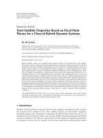
cuting the generalized RBF on a sinusoidal chirp signal with
a variable frequency of 300 to 305 Hz is shown in Figure 5.
As shown in Figure 5(a), the output and the desired value in
response to the narrow band signal has lower error, but this
network is not able to lear n the duct output in the broad-
band spectrum of the input signal of Figure 5(b), while the
proposed algorithm gives better results.
Two networ ks are com pared in Figure 6. The error norm
of the proposed algorithm compared to the GRBF in duct
identification is improved 94%. Hence, in identifying a sys-
tem, the proposed system can be utilized. Several reasons can
be mentioned for superiority of this system relative to the
GRBF as follows.
(a) Using a filter bank instead of filter.
(b) Using N buffered samples of data instead of a single
stream of data.
(c) General and local consideration of data, that is,
buffered data.
(d) Increasing the network capacity by increasing the α

coefficient.
400 410 420 430 440 450 460 470 480
Samples
0.4
0.3
0.2
0.1
0
0.1
0.2
0.3
0.4
0.5
Amplitude
(a)
1955 1960 1965 1970 1975
Samples
1
0.5
0
0.5
1
Amplitude
GRBF
output
Desired signal
(b)
Figure 5: Part of the GRBF output and duct output in response to a
sinusoidal chir p signal with a variable frequency (a) 300 to 305 Hz,
(b) 200 to 500 Hz.

4.3. Active noise cancellation using
the proposed algorithm
After identifying the duct with the GRBF network, we pro-
ceed canceling the noise in the duct by the structure pre-
sented in Figure 3 . The learning curve of the execution result
on variable chirp sinusoid of 300–305 Hz for the proposed
network in comparison to the FX-LMS algorithm is given in
Figure 7.
For this purpose, first the duct is identified by the gener-
alized RBF for excitation frequencies of 200 to 500 Hz, then
αs are calculated in the proposed network by the normal-
ized LMS (NLMS) algorithm. Higher convergence speed and
lower error for the proposed algorithm in comparison to the
FX-LMS algorithm in Figure 7 are observed. On average, the
convergence speed has been increased 3 times and the final
MSE minimum error is decreased 30%.
Hadi Sadoghi Yazdi et al. 5
1540 1545 1550 1555 1560 1565
Samples
0.8
0.6
0.4
0.2
0
0.2
0.4
0.6
0.8
Amplitude
GRBF

output
Desired and output of
proposed system
(a)
0 200 400 600 800 1000 1200 1400 1600 1800
Samples
250
200
150
100
50
0
Learning curve
Error (dB)
(b)
Figure 6: (a) Comparison of t he RBF network output and the
proposed algorithm in identifying the duct in response to a sinu-
soidal chirp input of variable frequency 200–500 Hz. (b) The learn-
ing curve of the proposed algorithm in duct identification.
5. CONCLUSIONS
The process of canceling the acoustic noise in a duct has a
nonlinear nature. Therefore, linear adaptive filters such as
LMS are not able to actively cancel the noise. Due to the good
tracking capability of the LMS filter in a noisy environment,
the FX-LMS has been presented as a basic method in ANC
which models some what the nonlinear nature of the duct. In
this paper, by modeling the duct using the generalized RBF
neural network, it is possible to suppress the narrow band
variable frequency noise in the duct in a b etter way than the
FX-LMS method. The proposed method in comparison to

the FX-LMS algorithm is more than three times faster and
has 30% less error. Also, the change in the input frequency
0 500 1000 1500 2000 2500
Samples
250
200
150
100
50
0
Learning curve
Error (dB)
FX-LMS
algorithm
The proposed
method
Figure 7: The learning curve to sinusoidal chirp with variable fre-
quency of 300 to 305 Hz for the proposed system and the FX-LMS
algorithm.
causes the divergence, which the proposed method converges
as well.
In the proposed method, first the duct is identified by the
GRBF neural network and using a linear adaptive combiner
at their outputs, online identification of the nonlinear system
becomes possible. The weights of the linear combiner are up-
dated using the normalized LMS algorithm.
APPENDIX
Theorem A.1. Assume that MSE
i
= E{e

2
} is the mean-square
error in the input space, then the MSE at Φ-space will be
smaller than the input space.
Proof. the mapping is according to
Y
= Φ(X), (A.1)
where Φ(X)
= [ϕ(x, c
1
), ϕ(x, c
2
), , ϕ(x, c
K
)] and we can
assume that ϕ(x, c
i
) = exp(−(x − c
i
)
2
/2σ
2
). In simple form
we can write ϕ(x, c
i
) = exp(−x
2
). By substituting e(k) =
x

m
(k) − x(k)inϕ(x, c
i
), x
m
(k) is the actual state of the sig-
nal, then we have
ϕ

x( k), c
i

=
exp

−x(k)
2

= exp

−

x
m
(k)+e(k)

2

=
exp


−
x
m
(k)
2

exp

−
e
m
(k)
2

exp

−
2e
m
(k)x
m
(k)

.
(A.2)
Assuming e
m
(k)issmallenough,wecanbetake
exp(

−e
m
(k)
2
) term. Also we know that exp(−x
m
(k)
2
) is the
desired output in each dimension at the Φ-space. For simpli-
fication, we substitute y
= ϕ(x(k), c
i
), thus we have
y
= y
m
exp

−2e
m
(k)x
m
(k)

,(A.3)
6 EURASIP Journal on Advances in Signal Processing
where y
m
= e(−x

m
(k)
2
). The Taylor series expansion of term
exp(
−2e
m
(k)x
m
(k)) is
exp

−2e
m
(k)x
m
(k)

∼
=
1 − 2e
m
(k)x
m
(k),
y
= y
m
− 2e
m

x
m
y
m
= y
m
− 2e
m
x
m
e
−x
2
m
= y
m
− αe
m
.
(A.4)
The term α
= 2x
m
e
−x
2
m
is always smaller than one, or e
Φ
=

αe
m
,thuswehave
MSE
Φ
= E

e
2
Φ

=
α
2
E

e
2

,
MSE
Φ
= α
2
MSE
i
.
(A.5)
The above equation shows that MSE
Φ

< MSE
i
or “MSE
in Φ-space is smaller than MSE in the input space.”
REFERENCES
[1] S. M. Kuo and D. R. Morgan, “Active noise control: a tutorial
review,” Proceedings of the IEEE, vol. 87, no. 6, pp. 943–973,
1999.
[2] L. J. Eriksson, M. C. Allie, and R. A. Greiner, “The selection
and application of an IIR adaptive filter for use in active sound
attenuation,” IEEE Transactions on Acoustics, Speech, and Sig-
nal Processing, vol. 35, no. 4, pp. 433–437, 1987.
[3] L. J. Eriksson and M. C. Allie, “System considerations for
adaptive modelling applied to active noise control,” in Proceed-
ings of IEEE International Symposium on Circuits and Systems
(ISCAS ’88), vol. 3, pp. 2387–2390, Espoo, Finland, June 1988.
[4] M. Bouchard and Y. Feng, “Inverse structure for active noise
control and combined active noise control/sound reproduc-
tion systems,” IEEE Transactions on Speech and Audio Process-
ing, vol. 9, no. 2, pp. 141–151, 2001.
[5] S. J. Elliott and P. A. Nelson, “Active noise control,” IEEE Signal
Processing Magazine, vol. 10, no. 4, pp. 12–35, 1993.
[6] D. R. Morgan, “An analysis of multiple correlation cancellation
loops with a filter in the auxiliary path,” IEEE Transactions on
Acoustics, Speech, and Signal Processing, vol. 28, no. 4, pp. 454–
467, 1980.
[7] J. C. Burgess, “Active adaptive sound control in a duct: a com-
puter simulation,” JournaloftheAcousticalSocietyofAmerica,
vol. 70, no. 3, pp. 715–726, 1981.
[8] B. Rafaely, J. Carrilho, and P. Gardonio, “Novel active noise-

reducing headset using earshell vibration control,” Journal of
the Acoustical Society of America, vol. 112, no. 4, pp. 1471–
1481, 2002.
[9] M. Bouchard, B. Paillard, and C. T. Le Dinh, “Improved train-
ing of neural networks for the nonlinear active control of
sound and vibration,” IEEE Transactions on Neural Networks,
vol. 10, no. 2, pp. 391–401, 1999.
[10] L. S. H. Ngia and J. H. Sjoberg, “Efficient training of neu-
ral nets for nonlinear adaptive filtering using a recursive
Levenberg-Marquardt algorithm,” IEEE Transactions on Signal
Processing, vol. 48, no. 7, pp. 1915–1927, 2000.
[11] S. D. Snyder and N. Tanaka, “Active control of vibration us-
ing a neural network,” IEEE Transactions on Neural Networks,
vol. 6, no. 4, pp. 819–828, 1995.
[12] T. Wong, T. Lo, H. Leung, J. Litva, and E. Bosse, “Low-angle
radar tracking using radial basis function neural network,” IEE
Proceedings F: Radar and Signal Processing, vol. 140, no. 5, pp.
323–328, 1993.
[13] N. E. Longinov, “Predicting pilot look-angle with a radial ba-
sis function network,” IEEE Transaction on Syste ms, Man, and
Cybernetics, vol. 24, no. 10, pp. 1511–1518, 1994.
[14] S. Clen, “Nonlinear time series modelling and prediction us-
ing Gaussian RBF networks with enhanced clustering and RLS
learning,” Electronics Letters, vol. 31, no. 2, pp. 117–118, 1995.
[15] E. S. Chng, S. Chen, and B. Mulgrew, “Gradient radial basis
function networks for nonlinear and nonstationary time se-
ries prediction,” IEEE Transactions on Neural Networks, vol. 7,
no. 1, pp. 190–194, 1996.
[16] M. R. Berthold, “A time delay radial basis function network
for phoneme recognition,” in Proceedings of IEEE International

Conference on Neural Networks, vol. 7, pp. 4470–4472, 4472a,
Orlando, Fla, USA, June-July 1994.
[17] Z. Ryad, R. Daniel, and Z. Noureddine, “ The RRBF. Dynamic
representation of time in r adial basis function network,” in
Proceedings of 8th IEEE International Conference on Emerging
Technologies and Factory Automation (ETFA ’01), vol. 2, pp.
737–740, Antibes-Juan les Pins, France, October 2001.
[18] B. Sayyarrodsari, J. P. How, B. Hassibi, and A. Carrier, “An
estimation-based approach to the design of adaptive IIR fil-
ters,” in Proceedings of the American Control Conference, vol. 5,
pp. 3148–3152, Philadelphia, Pa, USA, June 1998.
[19] P. Lveg, “Process of silencing sound oscillations,” US Patent
no. 2043416, June, 1936.
[20] E. Bjarnason, “Analysis of the filtered-X LMS algorithm,” IEEE
Transactions on Speech and Audio Processing,vol.3,no.6,pp.
504–514, 1995.
[21] M. Rupp, “Saving complexity of modified filtered-X-LMS and
delayed update LMS algorithms,” IEEE Transactions on Circuits
and Systems II: Analog and Digital Signal Processing, vol. 44,
no. 1, pp. 57–60, 1997.
[22] S. M. Kuo, I. Panahi, K. M. Chung, T. Horner, M. Nadeski,
and J. Chyan, “Design of active noise control systems with the
TMS320 family,” Tech. Rep. SPRA042, Texas Instruments, Dal-
las, Tex, USA, 1996.
[23] S. K. Phooi, M. Zhihong, and H. R. Wu, “Nonlinear active
noise control using Lyapunov theory and RBF network,” in
Proceedings of the IEEE Workshop on Neural Networks for Signal
Processing, vol. 2, pp. 916–925, Sydney, NSW, Australia, De-
cember 2000.
[24] D. A. Cartes, L. R . Ray, and R. D. Collier, “Lyapunov turning of

the leaky LMS algorithm for single-source, single-point noise
cancellation,” Mechanical System and Signal Processing, vol. 17,
no. 5, pp. 925–944, 2003.
[25] S. Haykin, Neural Networks: A Comprehensive Foundation,
MacMillan College, New York, NY, USA, 1994.
Hadi Sadoghi Yazdi wasborninSabzevar,
Iran, in 1971. He received the B.S. degree in
electrical engineering from Ferdosi Mashad
University of Iran in 1994, and then he re-
ceived to the M.S. and Ph.D. deg rees in
electrical engineering from Tarbiat Modar-
res University of Iran, Tehran, in 1996 and
2005, respectively. He works in Engineering
Department as Assistant Professor at Tar-
biat Moallem University of Sabzevar. His re-
search interests include adaptive filtering, image and video process-
ing. He has more than 70 journal and conference publications in
subjects of interest areas.
Hadi Sadoghi Yazdi et al. 7
Javad Haddadnia works as an Assistant
Professor at Tarbiat Moallem University of
Sabzevar. He received the M.S. and Ph.D.
degrees in electrical engineering from Amir
Kabir University of Iran, Tehran, in 1999
and 2002, respectively. His research interests
include image processing.
Mojtaba Lotfizad was born in Tehran, Iran,
in 1955. He received the B.S. degree in elec-
trical engineering from Amir Kabir Univer-
sity of Iran in 1980 and the M.S. and Ph.D.

degrees from the University of Wales, UK,
in 1985 and 1988, respectively. He joined
the engineering faculty of Tarbiat Modarres
University of Iran. He has also been a Con-
sultant to several industrial and government
organizations. His current research interests
are signal processing, adaptive filtering , and speech processing and
specialized processors.