Báo cáo hóa học: " Research Article A Supervised Classification Algorithm for Note Onset Detection" ppt

Hindawi Publishing Corporation
EURASIP Journal on Advances in Signal Processing
Volume 2007, Article ID 43745, 13 pages
doi:10.1155/2007/43745
Research Article
A Supervised Classification Algorithm for
Note Onset Detection
Alexandre Lacoste and Douglas Eck
Department of Computer Science, University of Montreal, Montreal, QC, Canada H3T 1J4
Received 5 December 2005; Revised 9 August 2006; Accepted 26 August 2006
Recommended by Ichiro Fujinaga
This paper presents a novel approach to detecting onsets in music audio files. We use a supervised learning algorithm to classify
spectrogram frames extracted from digital audio as being onsets or nononsets. Frames classified as onsets are then treated with a
simple peak-picking algorithm based on a moving average. We present two versions of this approach. The first version uses a single
neural network classifier. The second version combines the predictions of several networks trained using different hyperparame-
ters. We describe the details of the algorithm and summarize the performance of both variants on several datasets. We also examine
our choice of hyperparameters by describing results of cross-validation experiments done on a custom dataset. We conclude that
a super vised learning approach to note onset detection performs well and warrants further investigation.
Copyright © 2007 Hindawi Publishing Corporation. All rights reserved.
1. INTRODUCTION
This paper is concerned with finding the onset times of notes
in music audio. Thoug h conceptually simple, this task is de-
ceivingly difficult to perform automatically with a computer.
Consider, for example, the na
¨
ıve approach of finding ampli-
tude peaks in the raw waveform. This strategy fails except
for trivially easy cases such as monophonic percussive in-
struments. At the same time, onset detection is implicated in
a number of important music information retrieval (MIR)
tasks, and thus warrants research. Onset detection is useful

in the analysis of temporal structure in music such as tempo
identification and mete r identification. Music classification and
music fingerprinting are two other relevant areas where on-
set detection can play a role. In the case of classification, on-
set locations could be used to significantly reduce the num-
ber of frame-level features retained. For example, a sampling
method could be used that preferentially selects from frames
near-predicted onset locations. A related segmentation strat-
egy for genre classification was used by West and Cox [1]. In
the case of music fingerprinting, onset times could be used
as the basis of a robust fingerprint vector.
Onset detection is also important in areas involving the
structured representation of music. For example, music edit-
ing (performed using, e.g., a sequencer) can be simplified
by using automatic onset detection to segment a waveform
into logical parts. Also, onset detection is fundamentally
important for the problem of automaticmusictranscription,
where a structured symbolic representation (usually a tradi-
tional music score) is inferred from a waveform.
Onsets detection algorithms can generally be divided into
three steps:
(1) transformation of the waveform to isolate different
frequency bands, in general, using either a filter bank or a
spectrogram,
(2) enhancement of bands such that note onsets are more
salient; this could involve, for example, a filter that detects
positive slopes,
(3) peak-picking to select discrete note onsets.
Our main focus is to explore how supervised learning
might be used to improve performance within this frame-

work. However, our investigation offers enhancements at
each of these three steps. In the first step, we look at different
methods for computing and representing the spectrogram as
well as at strategies for merging spectrogram frames. In the
second step—where we focus most of our attention—we in-
troduce a supervised approach that learns to identify rele-
vant peaks in the output of the first step. Specifically, we train
neural networks to provide the best possible onset trace for
the peak-picking part. In the third step, we take advantage
of a tempo estimate in order to integrate some aspects of
rhythmic struc ture into the peak-picking decision process.
In this paper, we first review the work done in this field
with special attention paid to another work done on onset
2 EURASIP Journal on Advances in Signal Processing
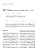
Music
source
Noise
source
Filter bank Filter bank
Envelope
extraction
Sum
Figure 1: Modulating noise with the energy envelope of different
bands from a filter bank retains the rhythmical content of the piece.
detection using machine learning. In Section 3,wedescribe
our algorithm including details about the simpler and more
complex variants. In Section 4, we describe a dataset that we
built for testing the model. Finally, in Section 5,wepresent
experiment results that report on our investigation of dif-
ferent spectrogram representations and on different network

architectures.
2. PREVIOUS WORK
Earlier algorithms developed for onset detection focused
mainly on the variation of the signal energy envelope in the
time domain. Scheirer [2] demonstrated that much informa-
tion from the signal can be discarded while still retaining the
rhythmical aspec t. On a set of test musical pieces, Scheirer
filtered out different frequency bands using a filter bank. He
extracted the energy envelope for each of those bands, us-
ing rectification and smoothing. Finally, with the same fil-
ter bank, he modulated a noisy signal with each of those
envelopes and merged everything by summation (Figure 1).
With this approach, rhythmical information was retained.
On the other hand, care must be taken when discarding in-
formation. In another experiment, he shows that if the en-
velopes are summed before modulating the noise, a signif-
icant amount of information about rhythmical structure is
lost.
Klapuri [3] used the psychoacoustical model developed
by Scheirer to develop a robust onset detector. To get better
frequency resolution, he employed a filter bank of 21 filters.
The author points out that the smallest detectable change in
intensity is proportional to the intensity of the signal. Thus
ΔI/I is a constant, where I is the signal’s intensity. Therefore,
instead of using (d/dt)A where A is the amplitude of the en-
velope, he used
1
A

d

dt
A

=
d
dt
log(A). (1)
This provides more stable onset peaks and allows lower in-
tensity onsets to be detected. Later, Klapuri e t al.used the
same kind of preprocessing [4] and won the ISMIR 2004
tempo induction contest [5].
2.1. Onset detection in phase domain
In contrast to Scheirer’s and Klapuri’s works, Duxbury et al.
[6–9] took advantage of phase information to track the on-
set of a note. They found that at steady state, oscillators tend
to have predictable phase. This is not the case at onset time,
allowing the decrease in predictability to be used as an indi-
cation of note onset. To measure this, they collected statis-
tics on the phase acceleration, as estimated by the following
equation:
α
k,n
= princarg

ϕ
k,n
− 2ϕ
k,(n−1)
+ ϕ
k,(n−2)


,(2)
where ϕ
k,n
is the kth frequency bin of the nth time frame
from the short-time Fourier transfor m of the audio signal.
The operator princarg maps the angle to the [
−π, π]range.
To detect the onset, different statistics were calculated across
the range of frequencies including mean, variance, and kur-
tosis. These provide an onset trace, which can be analyzed
by standard peak-picking algorithms. The authors also have
combined phase and energy on the complex domain for
more robust detection. Results on monophonic and poly-
phonic music show an increase in performance for phase
against energy, and even better performance when combin-
ing both.
2.2. Onset detection using supervised learning
Only a small amount of work has been done on mixing ma-
chine learning and onset detection. In a recent work, Kapanci
and Pfeffer [10] used a support vector machine (SVM) on
a set of frame features to estimate if there is an onset be-
tween two selected frames. Using this function in a hierar-
chical structure, they are able to find the position of onsets.
Their approach mainly focuses on finding onsets in signals
with slowly varying change over time such as solo singing.
Davy and Godsill [11] developed an audio segmentation
algorithm also using SVM. They classify spectrogram frames
into being probable onsets or not. The SVM was used to find
a hypersurface delimiting the probable zone from the less

probable one. Unfortunately, no clear test was made to out-
line the performance of the model.
Marolt et al. [12] used a neural network approach for
note onset detection. This approach is similar to ours in its
useofneuralnetworks,butisotherwiseverydifferent. The
model used the same kind of preprocessing as by Scheirer
in [2], with a filter bank of 22 filters. An integrate-and-fire
network was then applied separately to the 22 envelopes. Fi-
nally, a multi layer perceptron was applied on the output to
accept or reject the onsets. Results were good but the model
was only applied to monotimbral piano music.
3. ALGORITHM DESCRIPTION
In this section, we introduce two variants of our algor ithm.
Both use a neural network to classify frames as being on-
sets or nononsets. The first variant, SINGLE-NET, follows
A. Lacoste and D. Eck 3
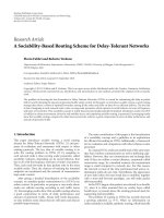
Song
Spectrogram
FNN
Peak picking
OST
Figure 2: SINGLE-NET flowchart. This simpler variant of our algo-
rithm is comprised of a time-space transform (spectrogram) w hich
is in turn treated with a feed-forward neural network (FNN). The
resulting trace is fed into a peak-picking algorithm to find onset
times (OSTs).
the process for onset detection described above and shown
in Figure 2. Our second var iant, MULTI-NET, combines in-
formation from (A) multiple instantiations of SINGLE-NET,
each trained with different hyperparameters and (B) tempo

traces gained by running a tempo-detection algorithm on the
neural network output vector. The multiple sources of evi-
dence are merged into a feature matrix similar to a spe ctro-
gram which is in turn fed back into another feed-forward
network, peak picker, and onset detector, see Figure 3.
3.1. Feature extraction
3.1.1. Time-frequency domain transform
Aside from the prediction of global tempo done in the
MULTI-NET variant of our algorithm, the information pro-
vided to the classification step of the algorithm is local in
time. This raises the question of how much local informa-
tion to integrate in order to achie ve best results. Using a pa-
rameter search, we concluded that a frame size of at least
50 milliseconds (1/20th of a second) was necessary to gener-
ate good results. For a sampling rate of 22050 Hz, this yields
∼ 1000 (22050/20) input values per frame for a supervised
learning algorithm.
As it is commonly done, we decided to use a time-space
transform to lower the dimensionality of the representa-
tion and to reveal spectral information in the signal. We fo-
cused on the short-time Fourier transform (STFT) and the
constant-Q transform [13]. These are discussed separately in
the following two sections.
3.1.2. Short-time Fourier transform (STFT)
The short-time Fourier transform is a version of the Fourier
transform designed for computing short-time duration
frames. A moving window is swept through the signal and
the Fourier transform is repeatedly applied to portions of the
signal inside the window
STFT(t, ω)

=

∞
−∞
x( τ)w
∗
(τ − t)e
−jωτ
dτ,(3)
Song
Repeat n times
Spectrogram
FNN1[i]
Find tempo
OST trace Tempo
Peak picking
Merge (2
n)
FNN2
OST
Figure 3: MULTI-NET flowchart. The SINGLE-NET var iant is re-
peated multiple times with different hyperparameters. A tempo-
detection algorithm is run on each of the resulting feed-forward
neural network (FNN) outputs. The SINGLE-NET outputs and the
tempo-detection outputs are then combined using a second neural
network.
where w(t) is the windowing function that isolates the signal
for a particular time t and where sequence x(t) is the signal
we want to transform, in this case, an audio signal in PCM
format.

The discrete version of the STFT is
STFT[n, k]
=
∞

m=−∞
x[ n + m]w[m]e
−jkm
. (4)
A Hamming window is applied to the signal. By choosing a
bigger window width, we get a better frequency resolution
but a smaller time resolution. Reducing the window width
produces the inverse effect.
3.1.3. Constant-Q transform
The constant-Q transform [13] is similar to the STFT but it
has two main differences:
(i) it has a logarithmic frequency scale;
(ii) it has a variable window width.
4 EURASIP Journal on Advances in Signal Processing
3.844.24.44.64.85
Time (s)
1.98
3.98
5.98
7.98
9.98
Frequency (KHz)
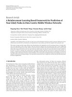
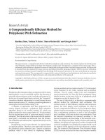
Figure 4: The magnitude plane of the STFT of a guitar record-
ing. The sampling frequency is 22050 Hz, the window width is
30 milliseconds, and the overlapping factor is 0.9. The dashed line

reveals the labeled onsets positions.
3.844.24.44.64.85
Time (s)
0.20
0.42
0.86
1.77
3.64
7.50
Frequency (KHz)
Figure 5: The magnitude plane of the constant-Q transform of the
same piece as in Figure 4. The sampling frequency is 22050 Hz, the
window width is 30 milliseconds, and the number of bins per octave
is 48. The dashed line reveals the labeled onset positions.
The logarithmic frequency scale provides a constant freq-
uency-to-resolution ratio for a particular bin,
Q
=
f
k
f
k+1
− f
k
=

2
1/b
− 1


−1
,(5)
where b represents the number of bins per octave and k the
frequency bin. For b
= 12, and by choosing a particular f
0
,
then k is equal to the MIDI note number (which represents
the equal-tempered 12-tone-per-octave scale). See Figure 5
for an example of a constant-Q transform.
As the frequency resolution is smaller at high frequencies,
we can shrink the window width to yield better time resolu-
tion, which is very important for onset detection.
Like the fast Fourier transform (FFT), there is an efficient
algorithm for constant-Q transform, see [14] for implemen-
tation details.
3.1.4. Phase planes
Both STFT and constant-Q are complex transforms. There-
fore, we can separate their outputs into phase and magnitude
planes. Obviously, the magnitude planes contain relevant in-
formation; see Figures 4 and 5. But can we do something with
33.544.55
Time (s)
1.48
2.98
4.48
5.98
7.48
8.98
10.48

Frequency (KHz)
Figure 6: The phase plane of the STFT calculated in Figure 4.Un-
manipulated, such a phase plane looks very much like a matrix of
noise.
344.24.44.64.85
Time (s)
1.98
3.98
5.98
7.98
9.98
Frequency (KHz)
Figure 7: The phase plane of the STFT of Figure 4,transformed
according to (2). The dashed line represents the labeled onsets po-
sitions. In this representation, the onset patterns are hard to see.
the phase plane? A visual observation (Figure 6) reveals that
the phase plane of an STFT is quite noisy.
One potentially useful way to process the phase plane
is according to (2). Exper iments from [8] show that the
probability distribution of phase acceleration over frequency
changes significantly at the moment of a note onset. How-
ever, in some cases, these onset patterns are almost absent, as
canbeseeninFigure 7. Our neural network was unable to
learn to find these patterns, see Tab le 1 for details.
So far, we have little evidence that the phase plane infor-
mation differentiated along the time axis will be useful in our
framework. However, the phase plane can also be differenti-
ated along the frequency axis (i.e., columnwise rather than
rowwise in the matrix),


k,n
= princarg

ϕ
k,n
− ϕ
(k−1),n

,(6)
where 
k,n
represents the phase difference between fr equency
bin k and frequency bin k
− 1 for a particular time bin
n. In many cases, this yields visible patterns that correlate
highly with onset times (Figure 8). This approach yields
more promising results within the framework of our model.
Tab le 1 shows that the frequency-differentiated phase plane
is able to perform almost as well as the magnitude plane.
A. Lacoste and D. Eck 5
Table 1: Results for running the FNN on different kinds of repre-
sentations. constant-Q performed the best, but the difference be-
tween Constant-Q and STFT is not significant. Phase acceleration
did slightly better than noise, and phase difference across frequency
yielded results almost as good as STFT.
Plane
Spectral
window size
F-meas. train F-meas. valid
STFT log mag 10 ms 86 ±2 86 ±5

STFT log mag
30 ms 86 ±1 86 ±5
STFT log mag
100 ms 84 ±2 83 ±8
C-Q log mag
10 ms 86 ±2 86 ±5
C-Q log mag
30 ms 87 ±2 87 ± 5
C-Q log mag
100 ms 84 ±2 84 ±6
STFT ph accel
10 ms 49 ±2 49 ±4
STFT ph accel
30 ms 47 ±1 47 ±5
STFT ph accel
100 ms 49 ±4 47 ±6
STFT ph freq-diff
10 ms 62 ±2 61 ±6
STFT ph freq-diff
30 ms 80 ±1 79 ±4
STFT ph freq-diff
100 ms 74 ±2 73 ±6
Noise
— 40 ±2 40 ±6
3.84 4.24.44.64.85
Time (s)
1.98
3.98
5.98
7.98

9.98
Frequency (KHz)
Figure 8: The phase plane of the STFT of Figure 4 transformed ac-
cording to (6). The dashed line represents the labeled onsets posi-
tions.
3.2. Supervised learning for onset emphasis
We employ a feed-forward neural network (FNN) to com-
bine evidence from the different transforms in order to clas-
sify the frames. Our goal is to use the neural net as a filter-
ing step in order to provide the best possible trace for the
peak-picking part. The network predicts the class member-
ship (onset or nononset) of each frame in a sequence. The ev-
idence available to the network for each prediction consists of
the different spectral features extra cted from the PCM signal
as described above. For a given frame, the network has an ac-
cess to the features for the frame in question as well as nearby
frames. In this section, we use the term “window” to refer to
the size of the input window defining which feature frames
are fed into the FNN. (This is in contr ast to the spectral
window used to calculate the spectrogram in Section 3.1.1.)
See Figure 9 for example.
3.84 4.24.44.64.85
Time (s)
0.41
0.84
1.72
3.54
7.29
Frequency (KHz)
Figure 9: The constant-Q transform of a piano musical piece with

labeled onsets. The dashed line is the onset trace, it corresponds to
the ideal input for the peak-picking algorithm. The red box is a win-
dow seen by the neural network for a particular time and particular
frequency. This input window has a width of 200 milliseconds.
3.2.1. Input variables
Onsets patterns are translation invariant on the time axis.
That is, the probability dist ribution over all the possible pat-
terns presented to the network does not depend on the time
value,
p

X = x | T = t

=
p(X = x), x ∈ R
n
,(7)
where n is the number of input variables, x represents a par-
ticular input to the network, and t is the central time of the
window.
Unfortunately, the frequency axis does not exhibit this
same shift invariance,
p

X = x | F = f

=
p(X = x), (8)
where f is the central frequency of the input window. For ex-
ample, when using the STFT, an onset with a fundamental at

a higher frequency will have more widely spaced harmonics
than a low-frequency onset. For the case of constant-Q trans-
form, the distances between harmonics are indeed shift in-
variant. However, for low frequencies, the patterns are highly
blurred over frequency and time.
Despite this, a small frequency shift introduces only small
changes in the underlying probability distributions,


f
1
− f
2


<  =⇒ p

x | f
1

 p

x | f
2

,(9)
where
 should be positive and relatively smal l.
As the spectrogram is not padded, the input window can
be translated only where it completely fits within the bound-

aries of the spectrogram. Thus, if we choose an input window
height of 100% of the spectrogram height, we have no possi-
bility for frequency translation at all. By reducing the window
height to 90% of the spectrogram height (Figure 9), we are
then able to make frequency translations that satisfy (9). For
example, if we have 200 frequency bins, the input window
will have a height of 180 frequency bins, and there will be 21
possible input window positions. For efficiency reasons, we
chose only 10 evenly spaced frequency positions. The goal
6 EURASIP Journal on Advances in Signal Processing
Table 2: Results for testing different input window sizes and differ-
ent numbers of input variables. Above the number of input vari-
ables is held constant at 200. Below the input window width is
held constant at 300 milliseconds. It is shown that the input win-
dow width is not crucial provided that i t is large enough. However,
the number of input variables is important.
Input window
width
No. input
F-meas. train F-meas. valid
variables
450 ms 200 86 ±2 86 ±6
300 ms
200 86 ±2 86 ±6
150 ms
200 86 ±2 86 ±5
75 ms
200 85 ±2 84 ±5
300 ms
100 84 ±2 84 ±6

300 ms
200 86 ±2 86 ±6
300 ms
400 87 ±2 87 ±5
300 ms
800 87 ±2 87 ±6
of performing translation over frequency is to have a smaller
input window, thus yielding fewer parameters to learn. This
strategy also provides multiple similar versions of the onset
trace, yielding a more robust model.
Unfortunately, even after frequency translation, there
were still too many variables in the input window to compute
efficiently. To address this, we used a random sampling tech-
nique. Input window values along the frequency axis were
sampled uniformly. However, sampling along the time axis
was done using a normal distribution centered at the onset
time. This strategy allowed us to concentrate our computa-
tional resources near the onset time. Table 2 shows results us-
ing different sampling densities. One hundred variables were
insufficient for optimal performance, but any value over 200
yielded good results.
3.2.2. Neural network structure
Our main goal is to use a supervised approach to enhance
the salience of onsets by learning from labeled examples. To
achieve this, we employed a feed-forward neural network
(FNN) with two hidden layers and a single neuron in the
output layer. The hidden layers used tanh activation func-
tions and the output layer used the logistic sigmoid activa-
tion function. Our choice of architecture was motivated by
general observations that multihidden layer networks may

offer better accuracy with fewer weights and biases than net-
works with single hidden layers. See Bishop [15,Chapter4]
for a discussion.
The performance for different network architectures is
shown in Section 5. Table 2 shows network performance for
different numbers of input variables and Tab le 3 shows per-
formance for different numbers of hidden units. A typical
structure uses 150 inputs variables, 18 hidden units in the
first layer, and 15 hidden units in the second layer.
Table 3: Results from tests using different neural network architec-
tures.
1st layer 2nd layer F-meas. train F-meas. valid
50 30 87 ±2 87 ±5
20
15 87 ±1 87 ±4
10
5 87 ±2 87 ±5
10
0 86 ±2 86 ±4
5
0 86 ±2 85 ±3
2
0 85 ±2 85 ±5
1
0 83 ±2 83 ±4
3.2.3. Target and error function
Recall that the goal of the network is to produce the ideal
trace for the peak-picking part. Such a target trace can be a
mixture of very peaked Gaussians, centered on the labeled
onset time,

T
s
(t) =

i
exp
−(τ
s,i
−t)
2
/σ
2
, (10)
where τ
s,i
is the ith labeled onset time of signal s and σ is the
width of the peak and is chosen to be 10 milliseconds.
The problem could also have been treated as a 0-1 on-
set/nononset classification problem. However, the abrupt
transitions between onset and nononset in the 0/1formu-
lation proved to be more difficult to model than the smooth
transitions provided by mixture of Gaussians.
For each time step, the FNN predicted the value given
by the target trace. The error function is the sum of squared
erroroverallpatterns,
E
=

s, j


T
s

t
j

−
O
s

t
j

2
, (11)
where O
s
(t
j
) is the output of the network for pattern j of
signal s.
3.2.4. Learning function
The learning function is the Polak-Ribiere version of conju-
gate gradient descent as implemented in the Matlab Neural
Network Toolbox.
To prevent the learner from overfitting, we employed the
commonly used regularization technique of early stopping.
In early stopping, learning is terminated when performance
worsens on a small out-of-sample dataset reserved for this
purpose [15].

We also used cross-validation. For more details on cross-
validation, see Section 5. For details on the dataset, see Sec-
tion 4.
3.3. Peak picking
The final step of our approach involves deciding which peaks
in our trace are to be treated as onsets. In our model, this
peak-picking process consists of three separate operations:
merging, peak ex traction,andthreshold opt imization.
A. Lacoste and D. Eck 7
2.53 3.54 4.55
Time (s)
0
0.2
0.4
0.6
0.8
1
Amplitude
Target trace
Onset trace
Figure 10: The target trace represents the ideal curve for the peak-
picking part of the algorithm. The onset trace shows the merged
output of the neural network.
3.3.1. Merging
As explained in Section 3.2.1, for reasons of robustness and
efficiency, an input window is applied to the spectrogram in
order to sample from a restricted range of frequencies. As this
window is moved up or down in frequency, multiple sets of
values for a single frame are generated. We process these sets
of values individually and merge their results by averaging,

generating a single onset trace, see Figure 10 for an example.
3.3.2. Peak extraction
To ensure that low-frequency trends in the sig n al do not dis-
tort peak height, we used a high-pass spatial filter to isolate
the high-frequency information of interest (including our
peaks). This high-pass filter was implemented subtractively:
we cross-correlated the signal using a Gaussian filter having
500 milliseconds of standard deviation. We then subtracted
this filtered version from the original signal, thus removing
low-frequency trends. Finally, we set to zero all values falling
below a threshold. These manipulations are expressed as fol-
lows:
ρ
s
(t) = O
s
(t) −u
s
(t)+K, (12)
where
u
s
(t) = g ∗O
s
(t), (13)
where g is the Gaussian filter, K is the threshold, and ρ
s
is the
peak trace of signal s. Using this approach, each zero crossing
with positive slope represents the beginning of an onset and

each zero crossing in a negative slope represents the end of
an onset.
The position of the onset is taken by calculating the cen-
ter of mass of all points inside the peak,
τ
s,i
=

j∈p
i
t
j
ρ
s

t
j


j∈p
i
ρ
s

t
j

, (14)
where τ
s,i

is the ith onset time of piece s and j is element of
all the points contained in peak i.
3.3.3. Threshold optimization
To optimize performance, the value of the threshold K in
(12) is learned using samples from the training set. In or-
der to make such an optimization, we require a way to gauge
the overall performance. For this, we adapt
1
the standard F-
measure to our task:
P
=
n
cd
n
cd
+ n
fp
, R =
n
cd
n
cd
+ n
fn
, F =
2PR
P + R
,
(15)

where n
cd
is the number of correctly detected onsets, n
fn
is
the number of false negatives, and n
fp
is the number of false
positives. A perfect score gives an F-measure of 1 and for a
fixed number of errors, the F-measure is optimal when the
number of false positives equals the number of false nega-
tives.
Since the peak-picking function is not continuous, we
cannot use gradient descent for optimization. The optimiza-
tion of noncontinuous values such a s K is usually achieved
using a line search algorithm like the golden section (see [16,
Section 10.1]). Fortunately, we have only one parameter to
optimize, thus making it possible to use a simpler method.
Specifically, we carried out a grid search over 25 values of
K where 0.02
≤ K ≤ 0.5 and retained the best performing
value.
3.4. MULTI-NET variant
Our exploration of input representations and neural network
architectures led us to the conclusion that there was no op-
timal set of hyperparameters for our SINGLE-NET model.
In an attempt to increase model robustness, we decided to
test a simple ensemble l earning approach by combining the
results of several SINGLE-NET learners trained with differ-
ent hyperparameters on the same dataset. In this section, we

describe the details of the resulting MULTI-NET model.
For the simulations described here, a MULTI-NET con-
sists of seven SINGLE-NET networks trained using different
hyperparameters. In addition, the SINGLE-NET networks
each benefited from a tempo trace calculated using predicted
onsets. An additional FNN was used to mix the results and to
derive a single prediction.
In raw p erformance terms, the additional complexity of
MULTI-NET seems warranted. For example, in the MIREX
2005 Contest (described briefly in Section 5.1), MULTI-NET
outperformed SINGLE-NET by 1.7% of F-measure and won
the first place. Details of the two major parts of MULTI-NET,
the tempo-trace computation and the merging procedure,
are explained in the following sections.
1
This F-measure was also used in the MIREX 2005 Audio Onset Detection
Contest.
8 EURASIP Journal on Advances in Signal Processing
2.53 3.544.55
Time (s)
0
0.2
0.4
0.6
0.8
1
Amplitude
Onset trace
Tem p o t race
Figure 11: The onset trace shows the merged output of the neu-

ral networks as in Figure 10. The tempo trace shows the cross-
correlation of the onset trace with its own autocorrelation.
3.4.1. Tempo trace
The SINGLE-NET variant has access only to short-timescale
information available from near-neighbor frames. As such,
it is unable to discover regularities that exist at longer
timescales. One important regularity is tempo. The rate of
note production is useful for predicting note onsets. For the
MULTI-NET variant, we calculate a tempo trace that can be
used to condition the probability that a particular point in
time is an onset.
To achieve this, we compute the tempo trace Γ by corre-
lating the interonset histogram of a particular point in the
onset trace with the inter-onset histogram of all other onsets.
If the two histograms are correlated, this indicates that this
point is in phase with the tempo,
Γ(t)
= h


μ
i
− μ
j

ij

·
h



μ
i
− t

i

, (16)
where Γ(t) is the tempo trace at time t, h(S) is the histogram
of set S,andμ
i
is the ith onset. The dot product between the
two histograms is the measure of correlation.
This method calculates n histograms, with each of them
requiring time O(n) to compute. Therefore, the algorithm is
O(n
2
). Moreover, if er rors occur in the peak extraction, they
directly affect the results of these histograms. To compensate
for this, Section 3.5 introduces a way to calculate the tempo
trace directly on the onset trace by computing the cross-
correlation of the onset trace with the onset trace’s autocorre-
lation. This yields an algorithm with complexity O(n log n),
see Figure 11 for an example.
3.4.2. Tempo-trace confidence
The tempo trace allows the final FNN to perform catego-
rization based not only on the ambiguity of a peak but also
on whether we are expect ing a peak or not at this particu-
lar time. In addition, we provide the network with the nor-
malized entropy of the interonset histogram as a measure of

rhythmicity,
H(T)
=
1
log
2
n
n

i=1
p

t
i

log
2
p

t
i

, (17)
where the normalization factor serves to map every measure
of entropy between 0 and 1. This provides the network with a
measure of confidence when weighing the relative influence
of the tempo.
3.4.3. Merging information
In order to merge information for the MULTI-NET variant
of our approach, we simply stack all the onset traces from our

multiple networks along with their tempo traces (including
the entropy-based prediction about rhythmicity). For exam-
ple, the 10 frequency translations with the onset trace and the
rhythmicity yield 12 traces p er model. Using 7 models gives
amatrixof84rows.
This merged information yields a matrix with a sampling
rate equal to the original spectrogram, but containing differ-
ent information. We continue with the SINGLE-NET variant
using this new feature frame in place of the orig inal spectro-
gram. Unlike the SINGLE-NET variant, the input window
takes into account 100% of the frequency spectr um. That is,
no sliding window over frequency is used because there is no
longer any continuity over frequency in the features we ex-
tracted.
3.5. Tempo trace by autocorrelation
In this section, we review autocorrelation and tempo induc-
tion. We then show that (16) can be calculated directly on the
onset trace by cross-correlating the signal with the autocor-
relation of the same signal.
3.5.1. Autocorrelation and tempo
The autocorrelation of a signal provides a high-resolution
picture of the relative salience of different periodicities, thus
motivating its use in tempo- and meter-related music tasks.
However, the autocorrelation transform discards all phase in-
formation, making it impossible to align salient periodicities
with the music. Thus autocorrelation can be used to pre-
dict, for example, that music has something that repeats ev-
ery 1000 milliseconds but it cannot say when the repetition
takes place relative to the start of the music.
Autocorrelation is certainly not the only way to com-

pute a tempo trace. Adaptive oscillator models [17, 18]can
be thought of as a time-domain correlate to autocorrelation
based methods and have shown promise, especially in cogni-
tive modeling. The integrate-and-fire neural network from
[12] can be viewed as such an oscillator-based approach.
Multiagent systems such as those by Dixon [19]havebeen
applied with success, as have Monte Carlo sampling [20]and
Kalman filtering methods [21].
Many researchers have used autocorrelation to find
tempo in music. Brown [22] was per haps the first to use au-
tocorrelation to find temporal structure in musical scores.
A. Lacoste and D. Eck 9
Scheirer [2] extended this work by treating audio files di-
rectly. Tzanetakis and Cook [23] used autocorrelation to gen-
erate a beat histogram as a feature for music classification.
They perform peak-picking as part of computing the beat
histogram, whereas peak-picking is our primary goal here.
Both Toiviainen and Eerola [24]andEck[25] used autocor-
relation to predict the meter in musical scores. Klapuri et
al. [4] incorporated the signal processing approaches of Goto
[26] and Scheirer in a model that analyzes the period and
phase of three levels of the metrical hierarchy. Eck [27] in-
troduced a method that combines the computation of phase
information and autocorrelation so that beat induction and
tempo prediction could be done directly in the autocorrela-
tion framework.
3.5.2. Tempo trace by autocorrelation
We will now prove that a tempo trace based on interonset
histograms can be calculated via autocorrelation. To start, let
us assume that the interonset histogram is equal to the au-

tocorrelation of the onset trace (in fact this is the case, as is
shown below),
h
a
(t) = γ  γ, (18)
where h
a
(t) is the interonset histogram for interonset time t,
γ is the original onset trace, and  is the cross-correlation
operator. Using this to rewrite (16)gives
Γ(t)
=

h
a
(t

)

γ  δ
t

dt

=

h
a
(t


)


γ(t

)δ(t

− t + t

)dt


dt

=

h
a
(t

)γ(t + t

)dt

= (γ  γ)  γ,
(19)
where Γ(t) is the tempo trace at time t and δ
t
≡ δ(τ − t),
where δ is the delta Dira c.

Therefore, the tempo trace can be calculated by correlat-
ing the onset tr ace 3 times w ith itself. This operation takes
now time O(n log n), which is much faster than the O(n
2
)re-
quired by (16).
3.5.3. Interonset histogram by autocorrelation
What remains is to demonstrate that the interonset his-
togram of a peaked trace is in fact equal to the autocorre-
lation of a p eaked trace. To achieve this, we first show that
the autocorrelation of the sum of a function is the pairwise
cross-correlation of all functions,
f (t)
≡

i
g
i
(t),
f (t)  f (t)
= F



F(k)


2

=

F


ij
G
i
(k)G
j
(k)

=

ij
g
i
(t)  g
j
(t),
(20)
where F(k)andG
i
(k) are, respectively, the results of the
Fourier transform of f (t)andg
i
(t). F is the Fourier trans-
form operat or.
It is a known result that the cross-correlation of two
Gaussians is another Gaussian with the new mean given by
μ
1

− μ
2
and the new variance is σ
2
1
+ σ
2
2
,
N

t; μ
1
, σ
1

 N

t; μ
2
, σ
2

=
N

t;

μ
1

− μ
2

,

σ
2
1
+ σ
2
2

,
(21)
where
N(t; μ, σ)
=
1
σ
√
2π
e
−(t−μ)
2
/σ
2
. (22)
If we approximate the onset trace as being a mixture of Gaus-
sians
γ(t)

=

i
α
i
N

t; μ
i
, σ
i

, (23)
then, using (20)and(23), we can rewrite the autocorrelation
of the onset traces
γ(t)  γ(t)
=

ij

α
i
N

t; μ
i
, σ
i




α
j
N

t; μ
j
, σ
j

(24)
and with (21), (24)becomes

ij
α
i
α
j
N

t;

μ
i
− μ
j

,

σ

2
i
+ σ
2
j

, (25)
which is a more general case of a Parzen window histogram.
The traditional case is where α
i
and σ
i
remain constant across
points. This loss of information occurs wh en we extract the
peaks from the onset trace, keeping only the position and ig-
noring the width and the height.
4. DATASET
To learn this task correctly, we needed a dataset with accurate
annotations that covers a wide variet y of musical styles. Ac-
curacy is particularly important for this task because tempo-
ral errors in mislabeling wil l have grave effects: the network
will be punished for predicting an onset at the correct posi-
tion and will be punished for not predicting an onset at the
erroneous position.
The most promising candidate dataset we found was a
publicly available collection from Leveau et al. [28]. Unfortu-
nately, this dataset was too small and restricted for our pur-
poses, mainly focusing on monophonic pieces.
We chose to annotate our own musical pieces. To make
it possible to share our annotations with others, we selected

the publicly available nonannotated “Ballroom” dataset from
ISMIR 2004 as a source for our w aveforms. The “Ballroom”
dataset is composed of 698 wav files of approximately 30 sec-
onds each. Annotating the complete dataset would be too
time consuming and was not necessary to train our model.
We therefore annotated 59 random segments of 10 sec-
onds each. Most of them are complex and polyphonic with
singing, mixed with pitched and noisy percussions.
The labels were manually annotated using a Matlab
program with GUI constructed by the first author to al-
low for precise annotation of wav files. The “Ballroom”
10 EURASIP Journal on Advances in Signal Processing
annotations as well as the Matlab interface are available
on request from the first author or at the following page:
/>∼lacostea
5. RESULTS
To choose among different methods and different hyperpa-
rameters, we tested the SINGLE-NET algorithm using 3 fold
cross-validation on the “Ballroom” dataset (Section 4). 15
pieces out of 69 were used for the test set and the 3 different
separations yield a measure of variance for b oth the training
and tests results.
A typical spectrogram contains 200 frames per second,
and each piece lasts 10 seconds. Taking into account the
10 frequency translations, this yields 20 000 input patterns
per piece. Learning from all of these patterns is redundant
and prohibitively slow. Thus we use only 5% of them, yield-
ing a total of 54 000 training examples. This in practice was
demonstrated to be enough data to prevent overfitting. The
dataset had an imbalanced ratio of onsets and nononsets

(positive and negative examples). In early training runs, we
tried sampling preferentially from frames near onsets. This
had no noticeable effect in the behavior of the model so for
later learning runs, including those discussed here, we did
not balance the training data.
For those tests, parameters not specified are assumed
to be the default as specified here: input window size is
150 milliseconds, sampling rate is 200 Hz, number of input
variables is 150, number of hidden units in layer one is 18,
number of hidden units in layer two is 15, and the Hamming
window size is 30 milliseconds.
The first test we made is to determine which plane is ap-
propriate for detecting onsets. We tested the logarithm of the
magnitude of the STFT, the logarithm of the amplitude of the
constant-Q transform, the phase acceleration, and the phase
difference along the frequency axis. For each of these, we
evaluated model performance for different window widths.
Tab le 1 shows the results for these tests. The b est perfor-
mance was achieved with the constant-Q transform, but the
difference between constant-Q and STFT is not significant.
The exact window width is not crucial provided it is small
enough. The phase acceleration performed only slightly bet-
ter than noise; however, the phase difference along frequency
axis worked much better, performing almost as well as the
STFT magnitude plane.
We then evaluated the input window width and the num-
ber of input variables on the magnitude plane of the STFT.
Tab le 2 shows that the input window width size is not crucial
provided that it is not too small. However, the number of in-
put variables is indeed important, with saturation occurring

at around 400.
In Table 3, we report performance results for different
network architectures. It can be seen that networks w ith two
hidden layers perform better than those having only a single
hidden layer. Also, it can bee seen that a relatively small num-
ber of neurons is sufficient for good performance (10 and
5 for the first and second layers, resp.). It is also interesting
Table 4: Results from tests combining STFT log-magnitude plane
with the phase difference across frequency plane as input to the
network. Unfortunately, the addition of phase difference in the fre-
quency axis does not yield better results than the STFT log magni-
tude alone.
No. input Hamming
window size
F-meas. train F-meas. valid
variables
100 30 ms 85 ±2 84 ± 5
100
50 ms 85 ±1 84 ±7
100
100 ms 80 ±2 79 ±8
200
30 ms 86 ±2 86 ±5
200
50 ms 86 ±2 85 ±6
200
100 ms 84 ±2 84 ±7
Table 5: Overall results of the MIREX 2005 onset detection contest
for our two variants. Their F-measures were the two highest. They
also had the best balance between the precision and recall. This is

probably due to to the learned threshold in the peak-picking part.
Vari ant MULTI-NET SINGLE-NET
Overall average F-measure 80.07% 78.35%
Overall average precision
79.27% 77.69%
Overall average recall
83.70% 83.27%
Tot al co rr ec t
7974 7884
Total false positives
1776 2317
Total false negatives
1525 1615
Tot al m erg ed
210 202
Tot al d oub le d
53 60
Runtime(s)
4713 1022
to note that a single neuron performs reasonably well (F-
measure of 83 versus 87 for our best performing model). This
suggests that it may be possible to constr u ct a simple, highly
efficient version of our model that can work on very large
datasets.
Tab le 1 suggests that combining the magnitude plane
with the phase plane might yield better results. In Table 4,we
report results from testing this idea using different numbers
of input variables and different Hamming window sizes. In
the table, the number of input variables corresponds to the
number of points for each plane. Unfortunately, the combi-

nation of magnitude plane with phase plane does not yield
better results.
5.1. MIEX 2005 results
Both variants of our algorithm were entered in the MIREX
2005 Audio Onset Detection Contest. The MIREX 2005
dataset is composed of 30 solo drum pieces, 30 solo mono-
phonic pitched pieces, 10 solo polyphonic pitched pieces,
and 15 complex mixes. On this dataset, the MULTI-NET al-
gorithm performed slightly better than the SINGLE-NET al-
gorithm. MULTI-NET yielded an F-measure of 80.07% while
SINGLE-NET yielded an F-measure of 78.35% (see Ta ble 5).
These results yielded the best and second best performance,
respectively, for the contest. See Ta ble 6 for results.
A. Lacoste and D. Eck 11
Table 6: Overall scores from the MIREX 2005 audio onset detection contest. Overall average F-measure, overall average precision, and
overall average recall are weighted by number of files in each of nine classes.
Rank Participant Avg. F-measure Avg. precision Avg. recall
1 Lacoste & Eck (MULTI-NET) 80.07% 79.27% 83.70%
2
Lacoste & Eck (SINGLE-NET) 78.35% 77.69% 83.27%
3
Ricard, J. 74.80% 81.36% 73.70%
4
Brossier, P. 74.72% 74.07% 81.95%
5
R
¨
obel,A.(2) 74.64% 83.93% 71.00%
6
Collins, N. 72.10% 87.96% 68.26%

7
R
¨
obel,A.(1) 69.57% 79.16% 68.60%
8
Pertusa, Klapuri, & I
˜
nesta 58.92% 60.01% 61.62%
9
West, K. 48.77% 48.50% 56.29%
Table 7: F-measure percentages for all nine classes from the MIREX 2005 audio onset detection contest. Best per formance for each class is
shown in bold. The number of pieces for each class is shown in parentheses.
Complex
Poly- Bars and
Brass Drum
Plucked Singing Sust.
Wind
(15)
pitched bells
(2) (30)
string voice strings
(4)
(10) (4) (9) (5) (6)
MULTI-NET 78.85 86.31 86.55 70.25 91.40 81.84 45.33 56.68 58.75
SINGLE-NET
77.02 85.93 86.37 67.88 89.91 83.49 34.35 52.87 56.48
Ricard, J.
71.90 83.26 87.17 72.66 90.97 77.85 27.59 38.45 38.57
Brossier, P.
76.16 80.88 73.97 64.88 86.28 79.99 22.16 57.92 52.08

R
¨
obel, A. (2)
62.84 76.24 90.34 68.32 89.96 84.20 40.68 36.18 66.01
Collins, N.
60.25 75.70 99.28 69.09 92.31 81.97 29.34 14.74 47.57
R
¨
obel, A. (1)
59.76 69.29 97.92 61.87 86.29 77.58 42.69 17.35 51.13
Pertusa et al.
50.16 59.37 60.22 54.41 77.22 67.74 11.12 38.45 25.59
West, K.
47.13 39.98 34.58 33.94 71.61 39.85 12.07 32.12 18.11
Both variants of the algorithm were designed to perform
well on a wide range of music, so they were less efficient
than other algorithms on monophonic pieces. But when al l
pieces are considered, MULTI-NET and SINGLE-NET were
the two best-performing entries in the contest. Both vari-
ants also showed a good balance between precision and re-
call. This advantage is likely due to the learned threshold in
the peak-picking part (Section 3.3).
6. DISCUSSION
An in-depth analysis of model errors on the annotated “Ball-
room” dataset shows that most of the false negatives are pro-
duced by pitched onsets with thin h armonics. This is sur-
prising because such onsets are easily perceived by human.
Our failure here is likely due to the fact that we only pick
a random subset of the variables from the input window.
Picking more variables helps, but for some pitched sounds

so few variables are responsible for coding the onset that
the FNN still fails. Incidentally, this perhaps explains why
our entry performed poorly on the category solo bars and
bells (see Table 7).WehadanF-measureof86.55% where
the best for this category was 99.28%. False positives, on the
other hand, were mainly generated by singing or vibrato, as
expected. But the algorithm is still quite robust for those
events.
There are also some boundary effects. At the beginning
and at the end of sequences, the network was often unable
to adequately resolve onsets. One solution to this problem
could be to train three different networks, one that predicts
onset using only information from the past, a second that
uses only information from the future, and a third one (like
the current model) that incorporates past and future frames.
For the first few frames, we could use the “future-only” ver-
sion, for the last frames, the “past-only” model and for all
other frames the “past-future” version. Moreover, the causal
“past-only” version could also be used for online detec-
tion.
On a more general note, we mentioned several tasks
that might benefit from good audio onset detection, such
as tempo detection, classification, and fingerprinting. This
is not to say that onset detection is required for tasks like
these. In fact, the MIR community seems mixed on the use-
fulness of onset detection in this domain: of the 13 entries
in the MIREX 2005 Tempo Contest, only 4 of them used de-
tected onsets or onset energy functions [29]. This may be due
to a philosophical rejection of onset detection as a part of
tempo finding. Scheirer [2] argued, for example, that explicit

note detection was not evident in the auditory system and
not necessary for tempo and beat analysis. However, it could
also be simply due to the fact that onset detection algorithms
have, to date, not worked very well. For example, this was the
12 EURASIP Journal on Advances in Signal Processing
main reason that the second author of this paper did not use
an onset detector in his MIREX entry [30].
6.1. Future work
Though our results are relatively good, there is still much
room for improvement. The ability to perform good pitch
detection would definitively improve model performance for
notes that have thin harmonics. Another way would be to
train a second network on a dataset of pitched onsets.
Different kinds of machine learning approaches can also
be used for this problem. Convolutional networks [31]would
be able to use a wider window and take advantage of all in-
put variables while still employing a reasonable amount of
parameters.
Working on a low-dimensional set of features instead of
the entire spectrogram could provide speed improvements
and could yield good results with a lower-capacity network.
This would allow us to train on a much larger annotated
dataset, perhaps yielding better generalization.
7. CONCLUSIONS
We have presented an algorithm that adds a supervised learn-
ing step to the basic onset detection framework of signal
transformation, feature enhancement, and peak picking. Our
SINGLE-NET variant used a sing le feed-forward neural net-
work to enhance spectrogram frames for peak picker. Our
MULTI-NET variant combined the predictions of several

SINGLE-NET networks with tempo traces to improve per-
formance. Though both models show promise, we believe
that the SINGLE-NET model warrants more attention due
to its relative simplicity. We provided evidence that our algo-
rithm works well, comparing it positively with other state-of-
the-art approaches. We conclude that the general approach of
supervised learning makes sense in the domain of audio note
onset detection.
APPENDIX
SUMMARY OF MIREX 2005 AUDIO ONSET
DETECTION RESULTS
The goal of the contest was to evaluate and compare on-
set detection algorithms applied to audio music record-
ings. The dataset consisted of 85 audio files (14.8 min-
utes total) from 9 classes: complex, polypitched, solo bars
and bells, solo brass, solo drum, solo plucked strings,
solo singing voice, solo sustained strings, and solo winds.
This information is summarized from ic-
ir.org/evaluation/mirex-results/audio-onset/index.html
REFERENCES
[1] K. West and S. Cox, “Finding an optimal segmentation for
audio genre classification,” in Proceedings of 6th International
Conference on Music Information Retrieval (ISMIR ’05),pp.
680–685, London, UK, September 2005.
[2] E. D. Scheirer, “Tempo and beat analysis of acoustic musical
signals,” Journal of the Acoustical Society of America, vol. 103,
no. 1, pp. 588–601, 1998.
[3] A. Klapuri, “Sound onset detection by applying psychoacous-
tic knowledge,” in Proceedings of IEEE International Conference
on Acoustics, Speech and Signal Processing (ICASSP ’99), vol. 6,

pp. 3089–3092, Phoenix, Ariz, USA, March 1999.
[4] A. P. Klapuri, A. J. Eronen, and J. T. Astola, “Analysis of the
meter of acoustic musical signals,” IEEE Transactions on Audio,
Speech and Language Processing, vol. 14, no. 1, pp. 342–355,
2006.
[5] F. Gouyon, A. Klapuri, S. Dixon, et al., “An experimental
comparison of audio tempo induction algorithms,” IEEE
Transactions on Audio, Speech and Language Processing, vol. 14,
no. 5, pp. 1832–1844, 2006.
[6] C.Duxbury,J.P.Bello,M.Davies,andM.Sandler,“Compled
domain onset detection for musical signals,” in Proceedings of
6th International Conference on Digital Audio Effects (DAFx
’03), London, UK, September 2003.
[7] C.Duxbury,J.P.Bello,M.Davies,andM.Sandler,“Acom-
bined phase and amplitude based approach to onset detection
for audio segmentation,” in Proceedings of the 4th European
Workshop on Image Analysis for Multimedia Interactive Services
(WIAMIS ’03), London, UK, April 2003.
[8] J.P.BelloandM.Sandler,“Phase-basednoteonsetdetection
for music signals,” in Proceedings of IEEE International Confer-
ence on Acoustics, Speech and Signal Processing (ICASSP ’03),
vol. 5, pp. 441–444, Hong Kong, April 2003.
[9] J.P.Bello,C.Duxbury,M.Davies,andM.Sandler,“Ontheuse
of phase and energy for musical onset detection in the complex
domain,” IEEE Signal Processing Le tters, vol. 11, no. 6, pp. 553–
556, 2004.
[10] E. Kapanci and A. Pfeffer, “A hierarchical approach to onset
detection,” in Proceedings of the International Computer Music
Conference (ICMC ’04), Miami, Fla, USA, October 2004.
[11] M. Davy and S. Godsill, “Detection of abrupt spectral changes

using support vector machines an application to audio signal
segmentation,” in Proceedings of IEEE International Conference
on Acoustics, Speech and Signal Processing (ICASSP ’02), vol. 2,
pp. 1313–1316, Orlando, Fla, USA, May 2002.
[12] M. Marolt, A. Kavcic, and M. Privosnik, “Neural networks for
note onset detection in piano music,” in Proceedings of the In-
ternational Computer Music Conference (ICMC ’02),Goten-
borg, Sweden, September 2002.
[13] J. C. Brown, “Calculation of a constant Q spectral transform,”
Journal of the Acoustical Society of America, vol. 89, no. 1, pp.
425–434, 1991.
[14] J. C. Brown and M. S. Puckette, “An efficient algorithm for the
calculation of a constant Q transform,” JournaloftheAcousti-
cal Society of America, vol. 92, no. 5, pp. 2698–2701, 1992.
[15] C. M. Bishop, Neural Networks for Pattern Recognition,Oxford
University Press, Oxford, UK, 1995.
[16] W. H. Press, S. A. Teukolsky, W. T. Vetterling, and B. P. Flan-
nery, Numerical Recipes in C: The Art of Scientific Computing,
Cambridge University Press, Cambridge, Mass, USA, 2nd edi-
tion, 1993.
[17] E. W. Large and J. F. Kolen, “Resonance and the perception of
musical met er,”
Connection Science, vol. 6, no. 1, pp. 177–208,
1994.
[18] D. Eck, “Finding downbeats with a relaxation oscillator,” Psy-
chological Research, vol. 66, no. 1, pp. 18–25, 2002.
A. Lacoste and D. Eck 13
[19] S. E. Dixon, “Automatic extraction of tempo and beat from ex-
pressive performances,” Journal of New Music Research, vol. 30,
no. 1, pp. 39–58, 2001.

[20] A. T. Cemgil and B. Kappen, “Monte Carlo methods for tempo
tracking and rhythm quantization,” Journal of Artificial Intelli-
gence Research, vol. 18, pp. 45–81, 2003.
[21] A. T. Cemgil, B. Kappen, P. W. M. Desain, and H. J. Honing,
“On tempo tracking: tempogram representation and Kalman
filtering,” Journal of New Music Research,vol.29,no.4,pp.
259–273, 2001.
[22] J. C. Brown, “Determination of the meter of musical scores by
autocorrelation,” Journal of the Acoustical Society of America,
vol. 94, no. 4, pp. 1953–1957, 1993.
[23] G. Tzanetakis and P. Cook, “Musical genre classification of au-
dio signals,” IEEE Transactions on Speech and Audio Processing,
vol. 10, no. 5, pp. 293–302, 2002.
[24] P. Toiviainen and T. Eerola, “The role of accent periodicities
in meter induction: a classificatin study,” in Proceedings of the
8th International Conference on Music Perception and Cognition
(ICMPC8 ’04), S. Lipscomb, R. Ashley, R. Gjerdingen, and P.
Webster, Eds., Causal Productions, Evanston, Ill, USA, August
2004.
[25] D. Eck, “A machine-learning approach to musical sequence in-
duction that uses autocorrelation to bridge long timelags,” in
Proceedings of the 8th Internat ional Conference on Music Per-
ception and Cognition (ICMPC8 ’04), S. D. Lipscomb, R. Ash-
ley, R. O. Gjerdingen, and P. Webster, Eds., Causal Produc-
tions, Evanston, Ill, USA, August 2004.
[26] M. Goto, “An audio-based real-time beat tracking system for
music with or without drum-sounds,” Journal of New Music
Research, vol. 30, no. 2, pp. 159–171, 2001.
[27] D. Eck, “Meter and autocorrelation,” in 10thRhythmPercep-
tion and Production Workshop (RPPW ’05),Blitzen,Belgium,

July 2005.
[28] P. Leveau, L. Daudet, and G. Richard, “Methodology and tools
for the evaluation of automatic onset detection algorithms in
music,” in Proceedings of 5th International Conference on Music
Information Retrieval (ISMIR ’04), Barcelona, Spain, October
2004.
[29] M. McKinney and D. Moelants, “Mirex 2005: tempo contest,”
in Proceedings of 6th International Conference on Music Infor-
mation Retrieval (ISMIR ’05), London, UK, September.
[30] D. Eck and N. Casagrande, “A tempo-extraction algo-
rithm using an autocorrelation phase matrix and shan-
non entropy,” MIREX tempo extraction contest, 2005,
/>[31] Y. LeCun and Y. Bengio, “Convolutional networks for images,
speech, and time-series,” in The Handbook of Brain Theory and
Neural Networks, M. Arbib, Ed., MIT Press, Cambridge, Mass,
USA, 1995.
Alexandre Lacoste received a B.S. degree in
physics and computer science (2004) from
the University of Montreal, where he is cur-
rently pursuing an M.S. degree in computer
science. His specialization is music and ma-
chine learning, with a focus on audio fea-
ture extraction and signal processing, su-
pervised learning, and web-based music in-
formation retrieval.
Douglas Eck completed a Ph.D. degree in
computer science and cognitive science at
Indiana University (2000). He is now an
Assistant Professor in the Department of
Computer Science at the University of Mon-

treal.HeisalsoanActiveMemberofBrain
Music and Sound BRAMS, an interdisci-
plinary group uniting music and brain re-
searchers from around Montreal. His pri-
mary area is machine learning in the do-
main of music, with focus on areas such as rhythm and meter, mu-
sic performance dynamics, and musical similarity in digital audio.