Báo cáo hóa học: "Research Article Pavement Crack Classification via Spatial Distribution Features" pptx

Hindawi Publishing Corporation
EURASIP Journal on Advances in Signal Processing
Volume 2011, Article ID 649675, 12 pages
doi:10.1155/2011/649675
Research Article
Pavement Crack Classification via Spatial Distribution Features
Qingquan Li,
1, 2
Qin Zou,
1, 2
and Xianglong Liu
1, 3
1
Transportation Research Center, Wuhan University, Wuhan 430079, China
2
School of Remote Sensing and Information Engineering, Wuhan University, Wuhan 430079, China
3
China Academy of Transportation Sciences, Ministry of Transport, Beijing 100013, China
Correspondence should be addressed to Qingquan Li,
Received 18 December 2010; Revised 26 February 2011; Accepted 8 March 2011
Academic Editor: Mark Liao
Copyright © 2011 Qingquan Li et al. This is an open access article distributed under the Creative Commons Attribution License,
which permits unrestricted use, distribution, and reproduction in any medium, provided the original work is properly cited.
Pavement crack types provide important information for making pavement maintenance str ategies. This paper proposes an
automatic pavement crack classification approach, exploiting the spatial distribution features (i.e., direction feature and density
feature) of the cracks under a neural network model. In this approach, a direction coding (D-Coding) algorithm is presented to
encode the crack subsections and extract the direction features, and a Delaunay Triangulation technique is employed to analyze
the crack region structure and extract the density features. As regarding skeletonized crack sections rather than cra ck pixels, the
spatial distribution features hold considerable feature significance for each type of cracks. Empirical study indicates a classification
precision of over 98% of the proposed approach.
1. Introduction

Pavement crack types are important for pavement dilapida-
tion analysis and pavement maintenance decision-making.
For asphalt pavements, the pavement cracks can generally
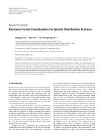
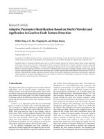
be classified into four types—the transverse crack, the
longitudinal crack, the block crack, and the alligator crack
[1] (see Figure 1). Each type of crack holds its own weight
in the pavement maintenance evaluation. Therefore, the
exploration of a robust and reliable approach for pavement
crack classification has great significance.
Over the past several decades, with the development
of high-speed cameras and large storage hardware, a real-
time collection of pavement images has been realized. While
along with the progress of image processing and pattern
recognition techniques, the image-based crack recognition
method gradually replaces the traditional manual method
and becomes a c ommon way for pavement crack detection
[2–7]. Pavement crack recognition includes two stages—
the crack detection and the crack classification. This paper
mostly focuses on the later.
Though a variety of approaches for pavement crack
classification have been proposed in the last two decades,
most of them cannot meet the requirements in practice
due to their inadequate consideration on spatial distribution
features of the cracks. For example, the projection histogram
methods [8–10] can be qualified to identify the directional
difference between cracks, but it may not be capable of
distinguishing the density difference. In a pavement image,
typically, a crack has a linear or curvilinear structure, the
spatial distribution of the crack points determines which
type of crack it is. Therefore, analyzing the crack’s spatial

distribution features, that is, the direction feature and density
feature, is the key point to crack classification. In this study,
a novel pavement crack classification approach is proposed
by using spatial distribution features in a neural network.
Under this approach, the problem of crack feature extraction
is formulated as the problem of direction and density feature
extraction on a binary skeletonized crack section. Generally,
the transverse and longitudinal cracks hold much more
direction features than the block and alligator cracks, while
the block and alligator cracks have more density features.
Moreover, the block cracks own less density features than
the alligator cracks. According to these characteristics of
the different crack types, we present a direction coding
algorithm (D-Coding) stemming from Freeman coding [11]
to acquire the direction features from skeletonized crack
sections, meanwhile we adopt the Delaunay Triangulation
2 EURASIP Journal on Advances in Signal Processing
(a) (b)
(c) (d)
Figure 1: The four types of pavement cracks. (a) The transverse, (b) the longitudinal, (c) the block, and (d) the alligator.
[12] technique to analyze the structure of the crack regions
and gain the density features of the crack. Experiments in our
research indicate the reliability of the extracted features.
The contributions of this paper are twofold: (1) a D-
Coding algorithm stemming from Freeman coding is pre-
sented for encoding the direction information of the linear
structures, and (2) the Delaunay Triangulation technique is
innovatively applied to analyze the crack region structure and
extract the crack density features.
The rest of this paper is organized as follows. Section 2

briefly gives the literature review of the related work
in pavement crack classification. Section 3 presents the
architecture of the proposed approach. Section 4 describes
our methodology in detail, which contains the singularity
points detection, linear subsection extraction, density fea-
ture expression, feature vector construction, and network
structure design. Section 5 gives the experimental results and
analysis, and Section 6 concludes our work by pointing out
future directions.
2. Previous Work
Inrecentyears,anumberofapproachesforpavementcrack
classification have been proposed which generally fall into
two categories—the supervised and the unsupervised. The
former includes a series of neural network-based approaches
[8–10, 13–19], while the later are rule-based approaches
[1, 20–22]. Among the neural network-based approaches,
Kaseko et al. [13] exploited a two-stage piecewise linear
neural network for crack classification and proved that it
outperforms the Bayes classifier and the k-nearest neighbor
(k-NN) classifier. In their study, five features were selected
to construct the class feature space: the number of crack
pixels in an image tile, the number of distressed pixels per
line in the transverse and longitudinal directions, and the
number of distressed pixels per line in the two diagonal
directions. Through crack primitives (i.e., crack sections)
analysis, Koutsopoulos et al. [14]extractedcrackfeatures
using the discriminant analysis, k-NN, and discrete choice
models. Some other approaches exploited the moment
features [15, 16]. Chou et al. [15] classified the pavement
distress based on Hu moments, Zemike moments, and

Bamieh moments, with a reported one-hundred percent
classification accuracy. Hsu et al. [16] used moment features
to classify real airport pavement distresses and gained an
accuracy of 85%. On the basis of extracting the geometric
and textural features, Sinha and Karray [17] constructed a
fuzzy neural classifier, and the declared precision is above
92.7%. Lee [8, 18] exploited three kinds of neural networks—
the image-based neural network (INN), the histogram-based
neural network (HNN), and the proximity-based neural
network (PNN). They divided the segmented image into
subimages firstly, tagged each sub-image into a crack tile
“1” or a noncrack tile “0”, thus forming a two-dimensional
Boolean crack matrix. After that, they summed this matrix
along the X and Y axes, forming two histogram vectors. Then
they tested three different feature extraction strategies on
these two vectors and demonstrated a best performance of
PNN of a classification accuracy of 95%. Considering the
density distribution difference between linear and regional
pavement distress, Xiao el al. [19] presented a density-
based neural network (DNN) classifier, and the claimed
precisions is above 99% to the simulated data and above
97% to the real pavement images. Rababaah et al. [9]
EURASIP Journal on Advances in Signal Processing 3
Pavement source
images
Pavement crack
sections
Binary skeletonized
crack sections
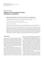
Architecture of the proposed approach

Linear subsection
extraction
Density feature
expression
Singularity points
detection
D-coding
Denaulay
triangulation
Direction feature
extraction
Density feature
extraction
Feature vector construction
Neural network classifier
Transverse
crack
Longitudinal
crack
Block crack
Alligator crack
Figure 2: The architecture of the proposed approach.
studied the projection features and Hough represented
features over three classifiers—the genetic algorithm (GA),
multilayer perceptrons (MLP), and self-organizing maps
(SOM). Experiments show the projection features are better
than the Hough represented features, and MLP is the best
classifier with an overall accuracy of 98.6%.
Among the unsupervised approaches, Georgopoulos
et al. [1] identified the crack type by analyzing the

geometrical properties of the cracks, which could also
generate the severity information. Considering the spatial
connectivity and directional consistency, Javidi et al. [20]
approached the pavement crack detection and classification
by a combination use of the wavelet multiscale edge detection
and the Hough transformation. It was reported to achieve
better results than the Wisecrax: a commercial product from
Roadware company. Wang et al. [21]presentedachain
coding algorithm to track the skeletonized cracks. Based on
the statistic parameters of the tracking array, they classified
the crack types. Beamlet transform-based approach was
proposed by Ying and Salari [22], where the sub-images are
represented with beamlets, based on which the segmentation,
linking, and classification operations are implemented.
Most of those methods mentioned above can obtain
certain accuracy under certain conditions such as noiseless
source images, limited experimental results, and computer
simulated experiment images. None of them have given
complete consideration to the spatial dist ribution features of
either direction or density.
3. Classification Framework
As has been discussed, the crack type is determined by the
spatial distribution features of the crack points. Therefore,
how to describe and generate the spatial distribution fea-
tures: the direction features and the density features is the key
point to the problem of pavement crack classification. The
direction features mainly contain four types: the transverse
direction (perpendicular to the road direction), longitudinal
direction (parallel to the road direction), and two diagonal
directions (with a 45

◦
or 135
◦
angle to the road direction).
The density features are depending on the number and
location of endpoints and junction points of the crack
sections. Considering the characteristics of these different
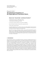
cracks, we propose the solution architecture shown in
Figure 2.
In order to extract spatial distribution features of the
cracks, we detect the singularity points on the binary skele-
tonized crack sections firstly, and then we introduce a direc-
tion coding (D-Coding) algorithm to compute the direction
information for each crack subsection generated from the
removal of singularity points. With singularity p oints, we
can also create the Delaunay triangles to analyze the crack
structure and extract the density features. Based on the D-
Coding results and Delaunay analyzing results, we construct
the feature vector with seven feature parameters. Finally, we
employ a BP (Back Propagation) neural network classifier
considering the feature vector and the classification output.
4. Methodology
We start this section with introducing the process of
singularity points detection, followed by a presentation of the
linear subsection extraction, and the Delaunay Triangulation
technique for density feature expression. Then we describe
the feature vector construction and the neural network
design.
4 EURASIP Journal on Advances in Signal Processing
(a) (b)

(c) (d)
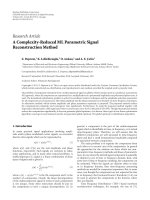
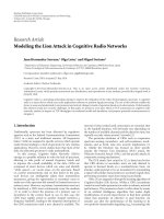
Figure 3: Basic singularity point structures. (a) and (b) the junction
point structures. (c) and (d) the endpoint structures. Note that the
center point is the target point concerned.
4.1. Singularity Points Detection. A pavement crack is com-
posed of linear subsections, and each subsection contains
two general endpoints: the endpoints and the junction
points. In this study, these two kinds of points are defined
as singularity points. With singularity points, the whole
pavement cr ack could be separated into several linear crack
subsections.
Exactly, there are two types of junction structures owing
to the centrosymmetric characteristic of the 8-connection
binary skeletonized crack sections. One is the intersection
with a transverse and a longitudinal line, and the other is
the intersection with two lines in diagonal directions, which
are illustrated in Figures 3(a) and 3(b), respectively. Also,
two types of basic endpoint structures are illustrated in
Figures 3(c) and 3(d). The first type includes points whose
8-connection neighborhood has only one crack p oint. The
other type includes points whose 8-connection neighbor-
hood contains one intersection point, while no other crack
points exist in its 8-connection neighborhood except the
ones belonging to the neighborhood of that intersection
point.
The singularity points of the crack skeletons are detected
based on the definitions and rules described above. Figure 4
illustrates the results of singularity point detection.
4.2. Linear Subsection Extraction Using D-Coding. In order to
express the spatial direction features of the crack, we divide

crack skeletons into linear crack subsections by removal of
the singularity points. As mentioned above, the direction
feature of the crack subsections is very important to linear
pavement distress classification.
On the basis of the classical 8-direction Freeman coding
and the centrosymmetric characteristic of the 8-connection
neighborhood, we propose a direction coding (D-Coding) to
encode the crack subsections. On the one hand, since crack
direction can be fully expressed by an angle between 0 to
180 degrees, we need only one direction code for one crack
line. On the other hand, as a crack line is an 8-connection
component, we cannot use a 4-direction encoding strategy,
for example, the 4-direction Freeman coding. Therefore,
we form our D-Coding structure by equalizing each two
codes in centrosymmetric in an 8-direction Freeman coding
structure. As illustrated in Figure 5, (a) is the conventional
diagram of the classical 8-direction Freeman coding, (b)
is for the 4-direction Freeman coding, and (c) is the
diagram of the D-Coding. Considering the convenience of
the subsequent analysis, the starting code begins with 1, and
withanorderof1,2,3,and4.AsFigure 5(c) illustrated,
codes 1 and 3 stand for the horizontal and vertical direction,
while codes 2 and 4 stand for the two diagonal directions.
To activate the proposed D-Coding, two rules are formed:
(1) to crack skeletons with junction points, the junction
points are regarded as the start coding points and (2) to crack
skeletons without junctions, the endpoints are regarded as
the coding start.
Given the starting code be set as 0, the corresponding D-
Coding results for cracks in Figures 4(e)–4(h) are shown in

Figure 6.
4.3. Density Feature Expression with Delaunay Triangles. The
singularity points also provide important clues for crack
density distribution features. The number and location of
the singularity points show the complexity of the crack, and
the structure of the crack region, which are highly related to
the density property of the cr ack, and vital for identifying a
crack’s type. In order to describe these density properties, we
apply the Delaunay Triangulation technique.
In mathematics and computational geometry, a Delau-
nay Triangulation for a set P of points in the plane is a
triangulation DT(P) such that no point in P is inside the
circumcircle of any triangle in DT(P). Delaunay Triangu-
lations maximize the minimum angle of all the angles of
the triangles in the triangulation; they tend to avoid skinny
triangles [23].
Delaunay triangles can be created based on the Delaunay
Graphs. Let P be a set of spatial points, DG(P) be the
Delaunay Graph of P, then DG(P) can be obtained through
the following two steps:
(i) calculate the Voronoi diagram of P,Vor(P),
(ii) place one vertex in each site of the Vor(P), if two sites
s
i
and s
j
share an edge, create an edge between v
i
and
v

j
,wherev
i
and v
j
are the vertices located in sites s
i
and s
j
,respectively.
Once D G( P) is obtained, the Delaunay Triangulation
DT(P) could be gained simply by replacing the graph edges
with lines.
With the singularity points detected in Section 4.1,
we could implement the Delaunay Triangulation for the
EURASIP Journal on Advances in Signal Processing 5
(a) (b) (c) (d)
(e) (f) (g) (h)
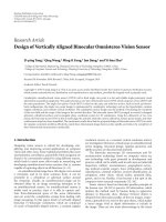
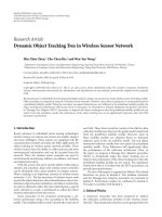
Figure 4: Examples for singularity point detection. Images (a–d) are computer simulated crack skeleton maps for the transverse crack, the
longitudinal crack, the block crack, and the alligator crack, respectively. Images (e–h) are the corresponding results for singularity point
detection, where the black points refer to the crack points, the blue ones denote the endpoints, and the yellow ones represent the junction
points.
0
123
4
567
(a)
0
1
2

3
(b)
11
2
23
3
4
4
(c)
Figure 5: D-Coding structure. (a) The 8-direction Freeman coding
structure, (b) the 4-direction Freeman coding structure, and (c) the
proposed D-Coding structure.
crack. Figures 7 and 8 illustrate the Voronoi diagram and
Delaunay triangles of Figures 4(g) and 4(h),respectively.
The circumcircle excluding and minimum-angle maximizing
properties of the Delaunay Triangulation make the Delaunay
triangles compactly describe the crack region structures,
which is helpful for representing the crack’s spatial densit y
features.
4.4. Feature Vector Constr uction. According to the definition
of different pavement cracks, the transverse and longitudinal
cracks have less singularity points, while the block and
alligator cracks have much more singularity points, especially
junction points. In addition, a transverse crack is abundant
in horizontal components, while a longitudinal crack is full
of vertical components. Moreover, the average area value
of the alligator crack regions is much smaller than that of
the block crack regions. Based on such above analysis, we
construct the feature vector as follows.
Let p

0
= n be the number of Delaunay triangles
generated from singularity points, let S
i
be the area value
of each triangle, and let a
j
( j ∈{1, 2,3, 4}) be the sum D-
coding value of the direction j segments, then the maximum
area value p
1
and the average area value p
2
of the triangles
can be formulized as (1)and(2), respectively
p
1
= max{S
i
| i = 1, 2, , n},
(1)
p
2
=

n
i
=1
S
i

n
.
(2)
The ratio d
j
( j ∈{1, 2, 3, 4})ofeachdirectioncom-
ponents which used to characterize the spatial distribution
direction features can be defined by
d
j
=
a
j

4
j
=1
a
j
. (3)
Then the feature vector P for pavement cracks classifica-
tion can be constructed as
P
=

p
0
, p
1
, p

2
, d
1
, d
2
, d
3
, d
4

T
. (4)
4.5. Neural Network Structure Design. The back-propagation
(BP) neural network is a typical multilayer feedforward
neural network which adjusts the weights and bias through
back propagation continuously until the Mean Square Error
(MSE) of the network tends to the least. It has been widely
applied to recognition, forecasting and procedure controlling
because of its strong abilities on nonlinear mapping, flexible
network structuring, and generalization. In this study, a
single hidden layer BP neural network is employed, and the
structure was designed as fol lows.
Let l be the input neurons number, let P (P
∈ R
l
) be the
input feature vector, let m be the number of hidden neurons,
Z (Z
∈ R
m

) be the middle hidden feature vector, let n be the
output neurons number, and let T (T
∈ R
n
) be the output
6 EURASIP Journal on Advances in Signal Processing
011
41 11 1111111
(a)
0
4
3
3
3
3
3
3
3
4
(b)
0
0
0
0
4
4
3
3
3
3

3
3
3
3
3
3
3
3
3
3
3
3
3
1
111
1
1
1
1
1
1
1
1
111
12
2
2
1111
1
11

(c)
0
00
0
000
0
00
0
00
0
0
3
3
3
3
3
3
3
3
3
3
3
3
3
3
3
3
3
3
3

3
3
3
3
3
3
3
3
3
3
3
3
3
3
3
3
3
3
3
3
3
3
3
3
3
3
11 11 11 11 1 1
1
1
11

11
1
11
1111
1
11111
11 11
(d)
Figure 6: The D-Coding results for four images in Figures 4(e)–4(h).
012345678910111213141516
0
1
2
3
4
5
6
7
8
9
10
11
12
(a) Voronoi diagram
012345678910111213141516
0
1
2
3
4

5
6
7
8
9
10
11
12
(b) Delaunay triangles
Figure 7: The Delaunay triangulation for Figure 4(g).
vector, then the feature vector space of each layer can be
described as follows:
P
=

p
1
, p
2
, , p
l

T
Input vector,
Z
=
(
z
1
, z

2
, , z
m
)
T
Hidden vector,
T
=
(
t
1
, t
2
, , t
n
)
T
Output vector.
(5)
Suppose that W
1
i, j
and b
1
j
are the connect weights and bias
value between input neurons p
i
(i ∈{0, 1, , l − 1})and
hidden neurons z

i
( j ∈{0, 1, , m − 1}), W
2
j,k
and b
2
k
are
the connect weights and bias value between hidden neuron
z
i
and output neuron t
k
(k ∈{0, 1, , n − 1}), then the
relationship of input layer, hidden layer and output layer can
be formulate as follows:
Z
j
= f
⎛
⎝
l−1

i=0
W
1
i, j
• P
i
+ b

1
j
⎞
⎠
,
T
k
= f
⎛
⎝
m−1

j=0
W
2
j,k
• Z
j
+ b
2
k
⎞
⎠
,
(6)
EURASIP Journal on Advances in Signal Processing 7
012345678910111213141516
0
1
2

3
4
5
6
7
8
9
10
11
12
(a) Voronoi diagram
012345678910111213141516
0
1
2
3
4
5
6
7
8
9
10
11
12
(b) Delaunay triangles
Figure 8: The Delaunay triangulation for Figure 4(h).
Transverse
Longitudinal
Block

Alligator
P[0]
P[1]
P[2]
P[3]
P[4]
P[5]
P[6]
Z[0]
Z[1]
.
.
.
Z[m
− 2]
Z[m
− 1]
T[0]
T[1]
T[2]
T[3]
Feature space
Input layer Hidden layer
Output layer
Figure 9: The neural network structure.
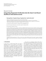
Camera
Figure 10: SmartV system.
where f (•) is the stimulation function. Based on the fact that
the input feature vector is a seven dimension space, while the
output patterns are with the transverse, longitudinal, block,

and alligator, the neuron numbers of the input layer and
Table 1: Feature values corresponding to the images in Figure 11.
Image
column
p
0
p
1
p
2
d
1
d
2
d
3
d
4
Column (a)
0 0.000 0.000 0.867 0.067 0.000 0.067
Column (b)
0 0.000 0.000 0.000 0.000 0.500 0.500
Column (c)
4 37.000 26.250 0.345 0.069 0.448 0.138
Column (d)
40 14.000 4.763 0.173 0.196 0.367 0.264
the output layer are set as l = 7andn = 4, respectively.
The suitable neurons number of the hidden layer m relies
on the repeated training results and is initially set as 30.
According to above description, the neural network structure

is illustrated by Figure 9.
5. Experimental Study
In this section, we first introduce the dataset used in this
study, and then give a real example for feature vector con-
struction. At last we examine and discuss the classification
details.
8 EURASIP Journal on Advances in Signal Processing
5.1. Dataset. A crack image database (SmartDB) containing
16000 image samples has been created based on 1200
pavement crack images captured by our SmartV system (see
Figure 10). Each type of cracks has 4000 samples, where the
crack type is labeled by two skilled workers and verified by an
expert. In order to evaluate the performance of the proposed
approach, the database images are divided into two batches,
one contains 8000 as the training sample images, and the
other contains 8000 as the testing sample images. Then, for
each type of crack, we have one 2000 images for training and
the other 2000 images for testing.
5.2. An Example for Feature Vector Construct ion with Real
Images. In order to illustrate the procedure of spatial
distribution feature extraction on cracks, four typical images
shown in Figure 11 (row 1) are selected to give a real example.
The results of each processing stage are arranged in rows. The
feature vector P of each crack image is extracted according
to the methods described in Section 4.4, and the feature
values corresponding to the four images are listed in Tabl e 1.
As mentioned in Section 4.4, p
0
is the number of triangles,
p

1
is maximum area value of the triangles, while p
2
is the
average area value, and d
j
( j ∈{1, 2,3, 4}) is the direction
components in four directions, respectively.
5.3. Evaluation. A series of training and testing experiments
were conducted under different number of hidden neurons
and different training epochs. Firstly, two metrics are
introduced for the result evaluation.
To a c r ack t y p e i (i
= 0, 1, 2, 3 denote the four types,
respectively), given a true-positive TP
i
, the number of cracks
which are correctly classified as type i, a false-positive FP
i
, the
number of cracks which are with type i but not classified as
type i, and a false-neg ative FN
i
, the number of cracks which
are incorrectly classified as type i, then the two objective
indices Precision
i
and Recall
i
are defined by [24]

Precision
i
=
TP
i
TP
i
+FP
i
,
Recall
i
=
TP
i
TP
i
+FN
i
.
(7)
Leting TP, FP, and FN denote the total number of the
corresponding cracks mentioned above, we have
TP
=
3

i=0
TP
i

,
FP
=
3

i=0
FP
i
,
FN
=
3

i=0
FN
i
.
(8)
Then the total Precision and Recall can be defined as
Precision
=
TP
TP + FP
,
Recall
=
TP
TP + FN
.
(9)

As each testing sample will be classified as one of the four
crack types, a false-positive in one type will certainly cause
a false-negative in another. Thus, we have FP
= FN, and
Precision
= Recall. We simply adopt one of them, for
example, Precision, to evaluate the overall performance.
Overall Performance. Taking the experimental strategies in
[16] for reference, we conduct the training and testing of
the constructed BP neural network under different hidden
neuron numbers from 30 to 120 at an interval of 30, and
under different epochs from 500 to 3000 at an interval of
500. The testing results are listed in Table 2.Ascanbeseen
from Table 2, we gains one of the best results (precision
=
98.038%) at epoch 2000 with 60 hidden neurons. Moreover,
the testing precision shows an ascending when the training
epoch increases from 500 to 2000, and a descending when
epoch increases from 2000 to 3000. It simply denotes that the
overfitting occurs when the epoch is over 2000. Therefore,
we select the best training model at an epoch of 2000 and a
hidden neuron number of 60.
Validity of the Proposed Feature Vector. To verify the reliabil-
ity of the presented feature vector, we compare it with three
feature vectors used in other approaches, one is the feature
vector based on the moments (Moments) [ 15, 16], and the
other two are feature vectors based on projection [9, 18].
All results shown in Table 3 are gained under an optimal
training epoch with 60 hidden neurons. The comparisons in
terms of precision and recall are also illustrated by Figure 12,

from which we can find that, the proposed feature vector
outperforms the other three competing feature vectors in
both precision and recall. Among the other three feature
vectors, the projection-based feature vector used in [9] gains
the most competing precision results with the proposed one,
however, it achieves much lower recalls in handling block and
alligator cracks.
Validity of the Selected Features. Also,weconductarange
of experiments to check the validity of the selected features.
To reach this, we construct the feature vector by excluding
each of the seven features in turn, and their performances
are illustrated in Figure 13.FromFigure 13,wecanfind
the feature vectors which have been element-excluded gains
lower a chie vements than the full-element feature vector,
which indicates the validity of e ach element of the proposed
feature vector. Meanwhile, we can see that, the features p
0
,
p
1
,andp
2
have high impact on results of the block and
alligator cracks, which denote their density characteristics.
And features d
1
and d
3
have high impact on results of
the transverse and l ongitudinal cracks, respectively, which

verifies their direction characteristics.
6. Conclusion
In this paper, we developed a new pavement crack classifi-
cation approach by using spatial distribution features of the
crack. In order to extract the direction distribution features,
we presented the D-Coding algorithm. While to extract
the density features, we adopt the Delaunay Triangulation
EURASIP Journal on Advances in Signal Processing 9
(1)
(2)
(3)
(4)
(5)
(a) (b) (c) (d)
Figure 11: Examples for spatial distribution features extraction. Row 1 shows the source pavement images with different crack types. Row
2 displays the corresponding binary skeletons of the crack sections. Row 3 gives the result images from the process of singularity point
detection, where the endpoints and junction points are labeled gray. Row 4 shows the D-Coding results of each crack subsections, in which
four gray level stands for four different kinds of direction code. Row 5 shows the Delaunay triangles generated from the singularity points.
10 EURASIP Journal on Advances in Signal Processing
Transverse Longitudinal Block Alligator
0.6
0.7
0.8
0.9
1
Crack type
Precision
Moments
Projection [18]
Projection [9]

Proposed
(a)
Recall
Transverse Longitudinal Block Alligator
0.6
0.7
0.8
0.9
1
Crack type
Moments
Projection [18]
Projection [9]
Proposed
(b)
Figure 12: Comparison of the four feature vectors. (a) Comparison on the Precision, (b) comparison on the Recall.
Table 2: Comparisons of testing results under different network parameters.
Epochs
Input-hidden-
output units
Transverse Longitudinal Block Alligator Total
FP FN FP FN FP FN FP FN FP FN Precision
500
7-30-4
164 179 158 182 175 172 197 161 694 694 91.325%
7-60-4
147 160 153 151 166 164 167 158 633 633 92.088%
7-90-4
133 141 138 146 153 154 157 140 581 581 92.738%
7-120-4

121 134 128 136 141 137 148 131 538 538 93.275%
1000
7-30-4
114 123 119 120 124 127 131 118 488 488 93.900%
7-60-4
102 112 114 113 110 115 121 107 447 447 94.413%
7-90-4
93 107 109 106 102 101 108 98 412 412 94.850%
7-120-4
86 100 106 99 93 90 97 93 382 382 95.225%
1500
7-30-4
89 94 101 87 85 95 83 82 358 358 95.525%
7-60-4
78 82 84 76 75 81 66 64 303 303 96.213%
7-90-4
61 58 67 59 61 68 52 56 241 241 96.988%
7-120-4
46 48 53 47 49 51 32 34 180 180 97.750%
2000
7-30-4
48 44 50 50 51 56 35 34 184 184 97.700%
7-60-4
41 39 46 43 42 46 28 29 157 157 98.038%
7-90-4
41 39 46 43 42 46 28 29 157 157 98.038%
7-120-4
41 39 46 43 42 46 28 29 157 157 98.038%
2500
7-30-4

48 44 51 50 53 59 35 34 187 187 97.663%
7-60-4
47 44 51 49 43 51 33 30 174 174 97.825%
7-90-4
44 39 48 47 42 47 28 29 162 162 97.975%
7-120-4
44 39 48 47 42 47 28 29 162 162 97.975%
3000
7-30-4
65 54 62 58 61 65 44 55 232 232 97.100%
7-60-4
54 51 58 56 60 62 42 45 214 214 97.325%
7-90-4
50 51 49 56 55 55 42 34 196 196 97.550%
7-120-4
46 45 51 51 45 46 30 30 172 172 97.850%
technique. Based on D-Coding results and Delaunay ana-
lyzing results, we calculated seven parameters to construct
the feature vector for input of a neural network classifier.
Considering skeletonized binary crack sections rather than
crack pixels, the proposed spatial distribution features well-
represent the characteristics of all four different types of
cracks. A wide range of experiments on real pavement images
proved the validity of the feature vector we constructed and
demonstrated an overall classification precision of above
98%.
Currently, the proposed approach can be further
improved. We will construct feature vectors by combining
EURASIP Journal on Advances in Signal Processing 11
Table 3: Performances of the four feature vectors.

Crack type
Moments Projection [18]Projection[9]Proposed
FP FN FP FN FP FN FP FN
Transverse 312 304 129 231 107 43 41 39
Longitudinal 224 307 170 258 110 50 46 43
Block 352 310 273 157 121 125 42 46
Alligator 316 283 286 212 16 136 28 29
0.3
0.4
0.5
0.6
0.7
0.8
0.9
1
Precision
All
p
0
excluded
p
1
excluded
p
2
excluded
d
1
excluded
d

2
excluded
d
3
excluded
d
4
excluded
Transverse
Longitudinal
Block
Alligator
Crack type
(a)
Recall
0.3
0.4
0.5
0.6
0.7
0.8
0.9
1
All
p
0
excluded
p
1
excluded

p
2
excluded
d
1
excluded
d
2
excluded
d
3
excluded
d
4
excluded
Transverse
Longitudinal
Block
Alligator
Crack type
(b)
Figure 13: Performance evaluation for the cross-validation processes. (a) Comparison on the Precision, (b) comparison on the Recall.
the selected features with features used in other approaches,
for example, the projection features. Moreover, we will study
other classifiers and other classification strategies in our
work.
Acknowledgments
This research is supported by the National Innovation
Team Foundation of China under Grant no. 40721001,
the Doctoral Research Programs of China under Grant

no. 20070486001, and the Chinese Fundamental Research
Funds for the Central Universities under Grant no.
20102130101000130.
References
[1] A. Georgopoulos, A. Loizos, and A. Flouda, “Digital image
processing as a tool for pavement distress evaluation,” ISPRS
Journal of Photogrammetry and Remote Sensing,vol.50,no.1,
pp. 23–33, 1995.
[2] T. Fukuhara, K . Terada, M. Nagao, A. Kasahara, and S. Ichi-
hashi, “Automatic pavement-distress-survey system,” Journal
of Transportation Engineering, vol. 116, no. 3, pp. 280–286,
1990.
[3] H. D. Cheng and M. Miyojim, “Automatic pavement distress
detection system,” Information Sciences, vol. 108, no. 1–4, pp.
219–240, 1998.
[4] H. D. Cheng and M. Miyojim, “Novel system for automatic
pavement distress detection,” Journal of Computing in Civil
Engineering, vol. 12, no. 3, pp. 145–152, 1998.
[5] K. C. P. Wang and W. Gong, “Real-time automated survey
system of pavement cracking in parallel environment,” Journal
of Infrastructure Systems, vol. 11, no. 3, pp. 154–164, 2005.
[6] M. T. Obaidat and S. A. Al-kheder, “Integration of geo-
graphic information systems and computer vision systems for
pavement distress classification,” Construction and Building
Materials, vol. 20, no. 9, pp. 657–672, 2006.
[7] S. N. Yu, J. H. Jang, and C. S. Han, “Auto inspection system
using a mobile robot for detecting concrete cracks in a tunnel,”
Automation in Construction, vol. 16, no. 3, pp. 255–261, 2007.
[8] B. J. Lee and H. D. Lee, “A robust position invariant artificial
neural network for digital pavement crack analysis,” in TRB

Annual Meeting, Washington, DC, USA, 2003.
[9] H. Rababaah, D. Vrajitoru, and J. Wolfer, “Asphalt pavement
crack classification: a comparison of GA, MLP, and SOM,”
in Proceedings of the Genetic and Evolutionary Computation
Conference (GECCO ’05), Washington, DC, USA, 2005.
[10] J. Bray, B. Verma, X. Li, and W. He, “A neural network
based technique for automatic classification of road cracks,”
in Proceedings of the International Joint Conference on Neural
Networks (IJCNN ’06), pp. 907–912, Vancouver, Canada, 2006.
[11] H. Freeman, “On the encoding of arbitrary geometric configu-
rations,” IRE Transactions on Electronic Computers, vol. 10, pp.
260–268, 1961.
12 EURASIP Journal on Advances in Signal Processing
[12] B. Delaunay, “Sur la sph
`
ere vide,” Izvestia akademii nauk SSSR,
Otdelenie Matematicheskikh i Estestvennykh Nauk, vol. 7, pp.
793–800, 1934.
[13] M.S.Kaseko,Z.P.Lo,andS.G.Ritchie,“Comparisonoftra-
ditional and neural classifiers for pavement-crack detection,”
Journal of Transportation Engineering, vol. 120, no. 4, pp. 552–
569, 1994.
[14] H. N. Koutsopoulos, V. I. Kapotis, and A. B. Downey,
“Improved methods for classification of pavement distress
images,” Transportation Research Part C, vol. 2, no. 1, pp. 19–
33, 1994.
[15] J. Chou, W. A. O’Neill, and H. D. Cheng, “Pavement
distress classification using neural networks,” in Proceedings
of the IEEE International Conference on Systems, Man and
Cybernetics, pp. 397–401, October 1994.

[16] C. J. Hsu, C. F. Chen, C. Lee, and S. M. Huang, “Airport
pavement distress image classification using moment invariant
neural network,” in Proceedings of the 22nd Asian Conference
on Remote Sensing, Singapore, 2001.
[17] S. K. Sinha and F. Karray, “Classification of underground
pipe scanned images using feature extraction and neuro-fuzzy
algorithm,” IEEE Transactions on Neural Networks, vol. 13, no.
2, pp. 393–401, 2002.
[18] B. J. Lee and H. D. Lee, “Position-invariant neural network
for digital pavement crack analysis,” Computer-Aided Civil and
Infrastructure Engineering, vol. 19, no. 2, pp. 105–118, 2004.
[19] W. X. Xiao, X. P. Yan, and X. Zhang, “Pavement distress
image automatic classification based on density-based neural
network,” in Proceedings of the 1st International Conference on
Rough Sets and Knowledge Technology (RSKT ’2006), pp. 685–
692, Chongqing, China, 2006.
[20] B. Javidi, J. Stephens, S. Kishk, T. Naughton, J. McDonald,
and A. Isaac, “Pilot for automated detection and classification
of road surface degradation features,” Tech. Rep. JHR 03-293,
Connecticut Transportation Institute, University of Connecti-
cut, 2003.
[21] C. F. Wang, A. M. Sha, and Z. Y. Sun, “Pavement crack
classification based on chain code,” in Proceedings of the Sev-
enth International Conference on Fuzzy Systems and Knowledge
Discovery (FSKD ’10), pp. 593–597, Yantai, Shandong, China,
2010.
[22] L. Ying and E. Salari, “Beamlet transform-based technique for
pavement crack detection and classification,” Computer-Aided
Civil and Infrastructure Engineering, vol. 25, no. 8, pp. 572–
580, 2010.

[23]M.D.Berg,O.Cheong,M.V.Kreveld,andM.Over-
mars, Computational Geometry: Algorithms and Applications,
Springer, New York, NY, USA, 2008.
[24] D. L. Olson and D. Delen, Advanced Data Mining Techniques,
Springer, New York, NY, USA, 1st edition, 2008.