Báo cáo hóa học: " Research Article Determining Vision Graphs for Distributed Camera Networks Using Feature Digests" pptx

Hindawi Publishing Corporation
EURASIP Journal on Advances in Signal Processing
Volume 2007, Article ID 57034, 11 pages
doi:10.1155/2007/57034
Research Article
Determining Vision Graphs for Distributed Camera
Networks Using Feature Digests
Zhaolin Cheng, Dhanya Devarajan, and Richard J. Radke
Department of Electrical, Computer, and Systems Engineering, Rensselaer Polytechnic Institute, Troy, NY 12180, USA
Received 4 January 2006; Revised 18 April 2006; Accepted 18 May 2006
Recommended by Deepa Kundur
We propose a decentralized method for obtaining the vision graph for a distributed, ad-hoc camera network, in which each edge
of the graph represents two cameras that image a sufficiently large part of the same environment. Each camera encodes a spatially
well-distributed set of distinctive, approximately viewpoint-invariant feature points into a fixed-length “feature digest” that is
broadcast throughout the network. Each receiver camera robustly matches its own features with the decompressed digest and
decides whether sufficient evidence exists to form a vision graph edge. We also show how a camera calibration algorithm that
passes messages only along vision graph edges can recover accurate 3D structure and camera positions in a distributed manner.
We analyze the performance of different message formation schemes, and show that high detection rates (> 0.8) can be achieved
while maintaining low false alarm rates (< 0.05) using a simulated 60-node outdoor camera network.
Copyright © 2007 Zhaolin Cheng et al. This is an open access article distributed under the Creative Commons Attribution License,
which permits unrestricted use, distr ibution, and reproduction in any medium, provided the original work is properly cited.
1. INTRODUCTION
The automatic calibration of a collection of cameras (i.e., es-
timating their position and orientation relative to each other
and to their environment) is a central problem in computer
vision that requires techniques for both detecting/matching
feature points in the images acquired from the collection
of cameras and for subsequently estimating the camera pa-
rameters. While these problems have been extensively stud-
ied, most prior work assumes that they are solved at a single
processor after all of the images have been collected in one

place. This assumption is reasonable for much of the early
work on multi-camera vision in which all the cameras are in
the same room (e.g., [1, 2]). However, recent developments
in wireless sensor networks have made feasible a distributed
camera network, in which cameras and processing nodes may
be spread over a wide geographical area, with no central-
ized processor and limited ability to communicate a large
amount of information over long distances. We will require
new techniques for correspondence and calibration that are
well suited to such distributed camera networks—techniques
that take explicit account of the underlying communication
network and its constraints.
In this paper, we address the problem of efficiently es-
timating the vision graph foranad-hoccameranetwork,in
which each camera is represented by a node, and an edge ap-
pears between two nodes if the two cameras jointly image a
sufficiently large part of the environment (more precisely, an
edge exists if a stable, accurate estimate of the epipolar ge-
ometry can b e obtained). This graph will be necessary for
camera calibration as well as subsequent higher-level vision
tasks such as object tracking or 3D reconstruction. We can
think of the vision graph as an overlay graph on the under-
lying communication graph, which describes the cameras that
have direct communication links. We note that since cameras
are oriented, fixed-aperture sensors, a n edge in the commu-
nication graph does not always imply an edge in the vision
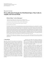
graph, and vice versa. For example, Figure 1 illustrates a hy-
pothetical network of ten cameras. We note that cameras E
and H, while physically proximate, image no common scene
points, while cameras C and F image some of the same scene

points despite being physically distant.
The main contribution of the paper is the description
and analysis of an algorithm for estimating the vision graph.
The key motivation for the algorithm is that we seek a de-
centralized technique in which a n unordered set of cameras
can only communicate a finite amount of information with
each other in order to establish the vision graph and mu-
tual correspondences. The underlying communication con-
straint is not usually a consideration in previous work on
2 EURASIP Journal on Advances in Signal Processing
A
B
C
D
E
F
G
H
J
K
(a)
A
B
C
D
E
F
G
H
J

K
(b)
A
B
C
D
E
F
G
H
J
K
(c)
Figure 1: (a) A snapshot of the instantaneous state of a camera network, indicating the fields of view of ten cameras. (b) A possible commu-
nication graph. (c) The associated vision graph.
image correspondence from the computer vision commu-
nity, but would be critical to the success of actual field im-
plementations of wireless camera networks. Each camera in-
dependently composes a fixed-length message that is a com-
pressed representation of its detected features, and broad-
casts this “feature digest” to the whole network. The basic
idea is to select a spatially well-distributed subset of distinc-
tive features for transmission to the broader network, and
compress them with principal component analysis. Upon re-
ceipt of a feature digest message, a receiver node compares
its own features to the decompressed features, robustly esti-
mates the epipolar geometry, and decides whether the num-
ber of robust matches constitutes sufficient evidence to es-
tablish a vision graph edge with the sender.
The paper is organized as follows. Section 2 reviews

prior work related to the estimation of v i sion graphs, and
Section 3 discusses methods from the computer vision lit-
erature for detecting and describing salient feature points.
Section 4 presents the key contribution of the paper, our
framework for establishing the vision graph, which includes
message formation, feature matching, and vision graph edge
detection. In Section 5, we briefly describe how the cam-
era network can be calibrated by passing messages along
established vision graph edges. The calibration approach
is based on our previously published work [3], which as-
sumed that the vision graph was given. The distributed
algorithm results in a metric reconstruction of the cam-
era network, based on structure-from-motion algorithms.
Section 6 presents a performance analysis on a set of 60
outdoor images. For the vision graph estimation algorithm,
we examine several tradeoffs in message composition in-
cluding the spatial distribution of features, the number of
features in the message, the amount of descriptor com-
pression, and the message length. Using receiver-operating-
characteristic (ROC) curves, we show how to select the fea-
ture messaging parameters that best achieve desired trade-
offs b etween the probabilities of detection and false alarm.
We also demonstrate the accurate calibration of the cam-
era network using the distributed structure-from-motion al-
gorithm, and show that camera positions and 3D struc-
tures in the environment can be accurately estimated. Finally,
Section 7 concludes the paper a nd discusses directions for fu-
ture work.
2. RELATED WORK
In this section, we review work from the computer vision

community related to the idea of estimating a vision graph
from a set of images. We emphasize that in contrast to the
work described here, communication constraints are gen-
erally not considered in these approaches, and that images
from all the cameras are typical ly analyzed at a powerful, cen-
tral processor.
Antone and Teller [4] used a camera adjacency graph
(similar to our v ision graph) to calibrate hundreds of still
omnidirectional cameras in the MIT City project. However,
this adjacency graph was obtained from a priori knowledge
of the cameras’ rough locations acquired by a GPS sensor,
instead of estimated from the images themselves. Similarly,
Sharp et al. [5] addressed how to distribute errors in esti-
mates of camera calibration parameters with respect to a vi-
sion graph, but this graph was manually constructed. We also
note that Huber [6] and Stamos and Leordeanu [7] consid-
ered graph formalisms for matching 3D range datasets. How-
ever, this problem of matching 3D subshapes is substantially
different from the problem of matching patches of 2D im-
ages (e.g., there are virtually no difficulties with illumination
variation or perspective distortion in range data).
Graph relationships on image sequences are frequently
encountered in image mosaicking applications, for example,
[8–10]. However, in such cases, adjacent images can be as-
sumed to have connecting edges, since they are closely sam-
pled frames of a smooth camera motion. Furthermore, a
chain of homog raphies can usually be constructed which
gives reasonable initial estimates for where other graph edges
occur. The problem considered in this paper is substantially
more complicated, since a camera network generally con-

tains a set of unordered images taken from different view-
points. The images used to localize the network may even be
acquired at different times, since we envision that a wireless
camera network would be realistically deployed in a time-
staggered fashion (e.g., by soldiers advancing through terr i-
tory or an autonomous unmanned vehicle dropping camera
nodes from the air), and that new nodes will occasionally be
deployed to replace failing ones.
A related area of research involves estimating the homo-
graphies that relate the ground plane of an environment as
Zhaolin Cheng et al. 3
imaged by multiple cameras. Tracking and associating ob-
jects moving on the ground plane (e.g., walking people) can
be used to estimate the visual overlap of camer as in the
absence of calibration (e.g., see [11, 12]). Unlike these ap-
proaches, the method described here requires neither the
presence of a ground plane nor the tracking of moving ob-
jects.
The work of Brown and colleagues [13, 14] represents
the state of the art in multi-image matching for the prob-
lem of constructing mosaics from an unordered set of im-
ages, though the vision graph is not explicitly constructed in
either case. Also in the unordered case, Schaffalitzky and Zis-
serman [15] used a greedy algorithm to build a spanning tree
(i.e., a partial vision graph) on a set of images, assuming the
multi-image correspondences were available at a single pro-
cessor.
An alternate method for distributed feature matching
than what we propose was described by Avidan et al. [16],
who used a probabilistic argument based on random graphs

to analyze the propagation of wide-baseline stereo matching
results obtained for a small number of image pairs to the
remaining cameras. However, the results in that work were
only validated on synthetic data, and did not extend to the
demonstration of camera calibration discussed here.
3. FEATURE DETECTORS AND DESCRIPTORS
The first step in estimating the vision graph is the detection
of hig h-quality features at each camera node– that is, regions
of pixels representing scene points that can be reliably, un-
ambiguously matched in other images of the same scene. A
recent focus in the computer vision community has been
on different types of “invariant” detectors that select image
regions that can be robustly matched even between images
where the camera perspectives or zooms are quite different.
An early approach was the Harris corner detector [17], which
finds locations where both eigenvalues of the local gradi-
ent matrix (see (1)) are large. Mikolajczyk and Schmid [18]
later extended Harris corners to a multiscale setting. An al-
ternate approach is to filter the image at multiple scales with
a Laplacian-of-Gaussian (LOG) filter [19]ordifference-of-
Gaussian (DOG) [20] filter; scale-space extrema of the fil-
tered image give the locations of the interest points. A broad
survey of modern feature detectors was given by Mikolajczyk
and Schmid [21]. As described below, we use difference-of-
Gaussian (DOG) features in our framework.
Once feature locations and regions of support have been
determined, each region must be described with a finite
number of scalar values—this set of numbers is called the
descriptor for the feature. The simplest descriptor is just a
set of image pixel intensities; however, the intensity values

alone are unlikely to be robust to scale or viewpoint changes.
Schmid and Mohr [22] proposed a descriptor that was in-
variant to the rotation of the feature. This was followed by
Lowe’s popular SIFT feature descriptor [20], which is a his-
togram of gradient orientations designed to be invariant to
scale and rotation of the feature. Typically, the algorithm
takes a 16
× 16 grid of samples from the gradient map at the
feature’s scale, and uses it to form a 4
× 4 aggregate gradient
matrix. Each element of the matrix is quantized into 8 orien-
tations, producing a descriptor of dimension 128. Baumberg
[23]andSchaffalitzky and Zisserman [15] applied banks of
linear filters to affine invariant support regions to obtain fea-
ture descriptors.
In the proposed algorithm, we detect DOG features and
compute SIFT descriptors as proposed by Lowe (see [20]).
Mikolajczyk and Schmid [24] showed that this combination
outperformed most other detector/descriptor combinations
in their experiments. As will be discussed in Section 4.1,we
also apply an image-adaptive principal component analysis
[25] to further compress feature descriptors.
4. THE FEATURE DIGEST ALGORITHM
When a new camera enters the network, there is no way to
know a priori which other network cameras should share
a vision graph edge with it. Hence, it is unavoidable that a
small amount of information from the new camera is dissem-
inated throughout the entire network. We note that there is
substantial research in the networking community on how to
efficiently deliver a message from one node to all other nodes

in the network. Techniques range from the naive method of
flooding [26] to more recent power-efficient methods such
as Heinzelman et al.’s SPIN [27]orLEACH[28]. Our focus
here is not on the mechanism of broadcast but on the ef-
ficient use of bits in the broadcast message. We show how
the most useful information from the new camera can be
compressed into a fixed-length feature message (or “digest”).
We assume that the message length is determined beforehand
based on communication and power constraints. Our strat-
egy is to select and compress only highly distinctive, spatially
well-distributed features which are likely to match features
in other images. When another camera node receives this
message, it will decide whether there is sufficient evidence
to form a vision graph edge with the sending node, based on
the number of features it can robustly match with the digest.
Clearly, there are tradeoffs for choosing the number of fea-
tures and the amount of compression to suit a given feature
digest length; we explore these tradeoffsinSection 6.Wenow
discuss the feature detection and compression algorithm that
occurs at each sending node and the feature matching and
vision graph edge decision algorithm that occurs at each re-
ceiving node in greater detail.
4.1. Feature subset selection and compression
The first step in constructing the feature digest at the send-
ing camera is to detect difference-of-Gaussian (DOG) fea-
tures in that camera’s image, and compute a SIFT descriptor
of length 128 for each feature. The number of features de-
tected by the sending camera, which we denote by N,isde-
termined by the number of scale-space extrema of the image
and user-specified thresholds to eliminate feature points that

have low contrast or too closely resemble a linear edge (see
[20] for more details). For a typical image, N is on the order
of hundreds or thousands.
4 EURASIP Journal on Advances in Signal Processing
(a) (b)
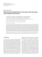
Figure 2: The goal is to select 256 representative features in the image. (a) The 256 strongest features are concentrated in a small area in the
image—more than 95% are located in the tree at upper left. (b) After applying the k-d tree partition with 128 leaf nodes, the features are
more uniformly spatially distributed.
The next step is to select a subset containing M of the
N features for the digest, such that the selected features are
both highly distinctive and spatially well-distributed across
the image (in order to maximize the probability of a match
with an overlapping image). We characterize feature distinc-
tiveness using a strength measure defined as follows. We first
compute the local gradient matrix
G
=
1
|W|
2
⎡
⎣

W
g
x
g
x

W

g
x
g
y

W
g
y
g
x

W
g
y
g
y
⎤
⎦
,(1)
where g
x
and g
y
are the finite difference derivatives in the
x and y dimensions, respectively, and the sum is computed
over an adaptive window W around each detected feature.
If the scale of a feature is σ, we found a window side of
|W|=
√
2σ to be a good choice that captures the impor-

tant local signal variation around the feature. We then define
the strength of feature i as
s
i
=
det G
i
tr G
i
,(2)
which was suggested by Brown et al. [14].
If the digest is to contain M features, we could just send
the M strongest features using the above strength measure.
However, in practice, there may be clusters of strong features
in small regions of the image that have similar textures, and
would u nfairly dominate the feature list (see Figure 2(a)).
Therefore, we need a way to distribute the features more
fairly across the image.
We propose an approach based on k-d trees to address
this problem. The k-d tree is a generalized binary tree that
has proven to be very effective for partitioning data in high-
dimensional spaces [29]. The idea is to successively partition
a dataset into rectangular regions such that each partition
cuts the region with the current highest variance in two, us-
ing the median data value as the dividing line. In our case, we
use a 2-dimensional k-d tree containing c cells constructed
from the image coordinates of feature points. In order to ob-
tain a balanced tree, we require the number of leaf nodes to
be a power of 2. For each nonterminal node, we partition the
node’s data along the dimension that has larger variance. The

results of a typical partition are shown in Figure 2(b). Finally,
we select the
M/c strongest features from each k-d cell to
add to the feature digest. Figure 2 compares the performance
of the feature selection algorithm with and without the k-d
tree. One can see that with the k-d tree, features are more
uniformly spatially distributed across the image, and thus we
expect that a higher number of features may match any given
overlapped image. This is similar to Brown et al.’s approach,
which uses adaptive non-maximal suppression (ANMS) to
select spatially-distributed multi-scale Harris corners [14].
Clearly, there will be a performance tradeoff between the
number of cells and the number of features per cell. While
there is probably no optimal number of cells for an arbitrary
set of images, by using a training subset of 12 overlapping
images (in total 132 pairs), we found that c
= 2
log
2
(M)
gave
the most correct matches.
Once the M features have been selected, we compress
them so that each is represented with K parameters (in-
stead of the 128 SIFT parameters). We do so by project-
ing each feature descriptor onto the top K principal com-
ponent vectors computed over the descriptors of the N
original features. Specifically, the feature digest is given by
{v, Q, p
1

, , p
M
,(x
1
, y
1
), ,(x
M
, y
M
)},wherev ∈ R
128
is
the mean of the N SIFT descriptors, Q is the 128
× K ma-
trix of principal component vectors, p
j
= Q
T
(v
j
− v) ∈ R
K
,
where v
j
is the jth selected feature’s SIFT descriptor ∈ R
128
,
and (x

j
, y
j
) are the image coordinates of the jth selected fea-
ture. Thus, the explicit relationship between the feature di-
gest length L, the number of features M, and the number of
principal components K is
L
= b

128(K +1)+M(K +2)

,(3)
where b is the number of bytes used to represent a real num-
ber. In our experiments, we chose b
= 4 for all parameters;
however, in the future, coding gains could be obtained by
adaptively varying this parameter. Therefore, for a fixed L,
Zhaolin Cheng et al. 5
(a) (b) (c)
(d) (e) (f)
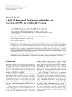
Figure 3: Example results of image matching from a pair of images. (a) Image 1. (b) Image 2. (c) The 1976 detected features in image 1.
(d) The k-d tree and corresponding 256-feature digest in image 1. (e) The dots indicate 78 features in image 1 detected as correspondences
in image 2, using the minimal Euclidean distance between SIFT descriptors and the ratio criterion with a threshold of 0.6. The 3 squares
indicate outlier features that were rejected. The circles indicate 45 new correspondences that were grown based on the epipolar geometry, for
a total of 120 correspondences. (f) The positions of the 120 corresponding features in image 2.
there is a tradeoff between sending many features (thus in-
creasing the chance of matches with overlapping images) and
coding the feature descriptors accurately (thus reducing false
or missed matches). We analyze these tradeoffsinSection 6.

4.2. Feature matching and vision graph edge detection
When the sending camera’s feature digest is received at a
given camera node, the goal is to determine whether a vision
graphedgeispresent.Inparticular,foreachsender/receiver
image pair where it exists, we want to obtain a stable, robust
estimate of the epipolar geometry based on the sender’s fea-
ture digest and the receiver’s complete feature list. We also
obtain the correspondences between the sender and receiver
that are consistent with the epipolar geometry, which are
used to provide evidence for a vision graph edge.
Based on the sender’s message, each receiving node gen-
erates an approximate descriptor for each incoming feature
as
v
j
= Qp
j
+ v. If we denote the receiving node’s features
by SIFT descriptors
{r
i
}, then we compute the nearest (r
1
j
)
and the second nearest (r
2
j
) receiver features to feature v
j

based on the Euclidean distance between SIFT descriptors in
R
128
. Denoting these distances d
1
j
and d
2
j
,respectively,weac-
cept (
v
j
, r
1
j
)asamatchifd
1
j
/d
2
j
is below a certain threshold.
The rationale, as described by Lowe [20], is to reject features
that may ambiguously match several regions in the receiv-
ing image (in this case, the ratio d
1
j
/d
2

j
would be close to 1).
In our experiments, we used a threshold of 0.6. However,
it is possible that this process may reject correctly matched
features or include false matches (also known as outliers).
Furthermore, correct feature matches that are not the clos-
est matches in terms of Euclidean distance between descrip-
tors may exist at the receiver. To combat the outlier problem,
we robustly estimate the epipolar geometry and reject fea-
tures that are inconsistent with it [30]. To make sure we find
as many matches as we can, we add feature matches that are
consistent with the epipolar geometry and for which the ratio
d
1
j
/d
2
j
is suitably low. This process is illustrated in Figure 3.
Based on the grown matches, we simply declare a vision
graph edge if the number of final feature matches exceeds a
threshold τ, since it is highly unlikely that a large number of
good matches consistent with the epipolar geometry occur
by chance. In Section 6, we investigate the effects of varying
the threshold on vision graph edge detection performance.
We note that it would be possible to send more features
for the same K and L if we sent only feature descriptors and
not feature locations. However, we found that being able to
estimate the epipolar geometry at the receiver definitely im-
proves performance, as exemplified by the number of accu-

rately grown correspondences in Figure 3(e).
Once the vision graph is established, we can use feed-
back in the network to refine edge decisions. In particular,
false vision graph edges that remain after the process de-
scribed above can be detected and removed by sending un-
compressed features from one node to another and robustly
6 EURASIP Journal on Advances in Signal Processing
estimating the epipolar geometry based on all of the available
information (see Section 6). However, such messages would
be accomplished via more efficient point-to-point communi-
cation between the affected cameras, as opposed to a general
feature broadcast.
5. CALIBRATING THE CAMERA NETWORK
Next, we briefly describe how the camera network can be cal-
ibrated, given the vision graph edges and correspondences
estimated above. We assume that the vision graph G
= (V , E)
contains m nodes, each representing a perspective camera de-
scribed by a 3
× 4matrixP
i
:
P
i
= K
i
R
T
i


I − C
i

. (4)
Here, R
i
∈ SO(3) and C
i
∈ R
3
are the rotation matrix and
optical center comprising the external camera parameters. K
i
is the intrinsic parameter matrix, which we assume here can
be written as diag( f
i
, f
i
,1),where f
i
is the focal length of the
camera. (Additional parameters can be added to the camera
model, e.g., principal points or lens distortion, as the situa-
tion warrants.)
Each camera images some subset of a set of n scene points
{X
1
, X
2
, , X

n
}∈R
3
. This subset for camera i is described
by V
i
⊂{1, , n}. The projection of X
j
onto P
i
is given by
u
ij
∈ R
2
for j ∈ V
i
:
λ
ij

u
ij
1

=
P
i

X

j
1

,(5)
where λ
ij
is called the projective depth [31].
We define the neighbors of node i in the vision graph as
N(i)
={j ∈ V | (i, j) ∈ E}. To obtain a distributed initial
estimate of the camera parameters, we use the algorithm we
previously described in [3],whichoperatesasfollowsateach
node i.
(1) Estimate a projective reconstruction based on the
common scene points shared by i and N(i) (these
points are called the “nucleus”), using a projective fac-
torization method [31].
(2) Estimate a metric reconstruction from the projective
cameras, using a method based on the dual absolute
quadric [32].
(3) Triangulate scene points not in the nucleus using the
calibrated cameras [33].
(4) Use RANSAC [34]torejectoutlierswithlargerepro-
jection error, and repeat until the reprojection error
for all points is comparable to the assumed noise level
in the correspondences.
(5) Use the resulting structure-from-motion estimate as
the starting point for full bundl e adjustment [35]. That
is, if
u

jk
represents the projection of the estimate

X
i
k
onto the estimate

P
i
j
, then a nonlinear minimization
problem is solved at each node i,givenby
min
{P
i
j
}, j∈{i,N(i)}
{
X
i
k
}, k∈∩V
j

j

k

u

jk
− u
jk

T
Σ
−1
jk

u
jk
− u
jk

,(6)
where Σ
jk
is the 2×2 covariance matrix associated with
the noise in the image point u
jk
. The quantity inside
the sum is called the Mahalanobis distance between
u
jk
and u
jk
.
If the local calibration at a node fails for any reason, a
camera estimate is acquired from a neighboring node prior
to bundle adjustment. At the end of this initial calibration,

each node has estimates of its own camera parameters P
i
i
as
well as those of its neighbors in the vision graph P
i
j
, j ∈
N(i).
6. EXPERIMENTAL RESULTS
We simulated an outdoor camera network using a set of 60
widely separated images acquired from a Canon PowerShot
G5 digital camera in autofocus mode (so that the focal length
for each camera is different and unknown), using an image
resolution of 1600
×1200. Figure 4 shows some example im-
ages from the test set. The scene includes several buildings,
vehicles, and trees, and many repetitive structures (e.g., win-
dows). A calibration grid was used beforehand to verify that
for this camera, the skew was negligible, the principal point
was at the center of the image plane, the pixels were square,
and there was virtually no lens distortion. Therefore, our
pinhole projection model with a diagonal K matrix is jus-
tified in this case. We determined the ground truth vision
graph manually by declaring a vision graph edge between
two images if they have more than about 1/8areaoverlap.
Figure 5 shows the ground truth expressed as a sparse ma-
trix.
We evaluated the performance of the vision graph gener-
ation algorithm using fixed message sizes of length L

= 80,
100 and 120 kilobytes. Recall that the relationship between
the message length L, the number of features M, and the
number of PCA components K is given by (3). Our goal here
is to find the optimal combination of M and K for each L.We
model the establishment of vision graph edges as a typical de-
tection problem [36], and analyze the performance at a given
parameter combination as a point on a receiver-operating-
characteristic (ROC) curve. This curve plots the probability
of detection (i.e., the algorithm finds an edge when there is
actually an edge) against the probability of false alarm (i.e.,
the algorithm finds an edge when the two images actually
have little or no overlap). We denote the two probabilities
as p
d
and p
fa
,respectively.Different points on the curve
are generated by choosing different thresholds for the num-
ber of matches necessary to provide sufficient evidence for
an edge. The user can select an appropriate point on the
ROC curve based on application requirements on the per-
formance of the predictor. Figure 6 shows the ROC curves
for the 80 KB, 100 KB, and 120 KB cases for different com-
binations of M and K. By taking the upper envelope of each
graph in Figure 6, we can obtain overall “best” ROC curves
for each L, which are compared in Figure 7.InFigure 7,we
also indicate the “ideal” ROC curve that is obtained by ap-
plying our a lgorithm using all features from each image and
no compression. We can draw several conclusions from these

graphs.
Zhaolin Cheng et al. 7
Figure 4: Sample images from the 60-image test set.
0 102030405060
60
50
40
30
20
10
0
Figure 5: The ground truth vision graph for the test image set. A
dot at (i, j) indicates a vision graph edge between cameras i and j.
(1) For all message lengths, the algorithm has good
performance, since high probabilities of detection can
be achieved with low probabilities of false alarm (e.g.,
p
d
≥ 0.8 when p
fa
= 0.05). As expected, the perfor-
mance improves with the message length.
(2) Generally, neither extreme of making the number of
features very large (the light solid lines in Figure 6)nor
the number of principal components very large (the
dark solid lines in Figure 6) is optimal. The best detec-
tor performance is generally achieved at intermediate
values of both parameters.
(3) As the message length increases, the detector per-
formances become more similar (since the message

length is not as limiting), and detection probability
approaches that which can be achieved by sending all
features with no compression at all (the upper line in
Figure 7).
To calibrate the camera network, we chose the vision
graph specified by the circle on the 120 KB curve in Figure 7,
at which p
d
= 0.89 and p
fa
= 0.08. Then, each camera on
one side of a vision graph edge communicated all of its fea-
tures to the camera on the other side. This full information
was used to reestimate the epipolar geometry relating the
camera pair and enabled many false edges to be detected and
discarded. The resulting sparser, more accurate vision graph
is denoted by the square in Figure 7,atwhichp
d
= 0.89
and p
fa
= 0.03. The correspondences along each vision
graph edge provide the inputs u
ij
required for the camera
calibration algorithm, as descr ibed in Section 5 .
The camera calibration experiment was initially per-
formed on the full set of 60 images. However, since the cal-
ibration algorithm has stricter requirements on image rela-
tionships than the vision graph estimation algorithm, not

all 60 cameras in the network were ultimately calibrated due
to several factors. Eight images were automatically removed
from consideration due to insufficient initial overlap with
other images, and seven additional images were eliminated
by the RANSAC algorithm since a minimum number of in-
liers for metric reconstruction could not be found. Finally,
five images were removed from consideration because a met-
ric reconstruction could not be obtained (e.g., when the in-
lier feature points were almost entirely coplanar). Conse-
quently, 40 cameras were ultimately calibrated.
The ground t ruth calibration for this collection of cam-
eras is difficult to determine, since it would require a precise
8 EURASIP Journal on Advances in Signal Processing
00.10.20.30.40.5
Probability of false alarm, p
fa
0.2
0.3
0.4
0.5
0.6
0.7
0.8
0.9
1
Probability of detection, p
d
K = 73, M = 78
K
= 52, M = 158

K
= 46, M = 198
K
= 41, M = 238
K
= 31, M = 358
(a)
00.10.20.30.40.5
Probability of false alarm, p
fa
0.2
0.3
0.4
0.5
0.6
0.7
0.8
0.9
1
Probability of detection, p
d
K = 82, M = 117
K
= 62, M = 197
K
= 55, M = 237
K
= 49, M = 277
K
= 38, M = 397

(b)
00.10.20.30.40.5
Probability of false alarm, p
fa
0.2
0.3
0.4
0.5
0.6
0.7
0.8
0.9
1
Probability of detection, p
d
K = 88, M = 156
K
= 69, M = 236
K
= 62, M = 276
K
= 56, M = 316
K
= 44, M = 436
(c)
Figure 6: ROC curves giving detection probability p
d
versus false
alarm probability p
fa

,whenmessagesoflength(a)80KB,(b)
100 KB, and (c) 120 KB are transmitted to establish the vision graph.
00.05 0.10.15 0.20.25 0.30.35 0.40.45 0.5
Probability of false alarm, p
fa
0.2
0.3
0.4
0.5
0.6
0.7
0.8
0.9
1
Probability of detection, p
d
80 KB
100 KB
120 KB
Ideal
Figure 7: Best achievable ROC curves for message lengths 80 KB,
100 KB, and 120 KB. These are obtained by taking the upper enve-
lope of each curve in Figure 6 (so each line segment corresponds to
adifferent choice of M and K). The “ideal” curve is generated by
applying our algorithm using all features from each image and no
compression.
survey of multiple buildings and absolute 3D localization
(both position and orientation) of each camera. However,
we can evaluate the quality of reconstruction both quan-
titatively and qualitatively. The Euclidean reprojection er-

ror, obtained by averaging the values of
u
jk
− u
jk
 for ev-
ery camera/point combination, was computed as 0.59 pixels,
meaning the reprojections are accurate to within less than a
pixel. Since the entire scene consists of many buildings and
cameras, visualizing the full network simultaneously is dif-
ficult. Figure 8 shows a subset of the distributed calibration
result centered around a prominent church-like building in
the scene (Figure 8(a)). To make it easier to perceive the re-
constructed structure, in Figure 8(b) we manually overlay a
building outline from above to indicate the accurate posi-
tion of a subset of the estimated points on the 3D structure.
For example, the roof lines can be seen to be parallel to each
other and perpendicular to the front and back walls. While
this result was generated for visualization by registering each
camera’s structure to the same frame, each camera really only
knows its location relative to its neighbors and reconstructed
scene points.
7. CONCLUSIONS AND FUTURE WORK
We presented a new framework to determine image rela-
tionships in large networks of cameras where communica-
tion between cameras is constrained, as would be realistic
in any w ireless network setting. This is not a pure com-
puter vision problem, but requires attention to and anal-
ysis of the underlying communication constraints to make
the vision algorithm’s implementation viable. We presented

Zhaolin Cheng et al. 9
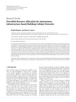
(a)
913
7
815
2
3
(b)
Figure 8: Camera calibration results for a prominent building in the scene. (a) Original image 2, with detected feature points overlaid. (b)
The 3D reconstruction of the corresponding scene points and several cameras obtained by the distributed calibration algorithm, seen from
an overhead view, with building shape manually overlaid. Parallel and per pendicular building faces can be seen to be correct. Focal lengths
have been exaggerated to show camera viewing angles. This is only a subset of the entire calibrated camera network.
algorithms for each camera node to autonomously select a
set of distinctive features in its image, compress them into a
compact, fixed-length message, and establish a vision graph
edge with another node upon receipt of such a message. The
ROC curve analysis gives insight into how the number of fea-
tures and amount of compression should be traded off to
achieve desired levels of performance. We also showed how
a distributed algorithm that passes messages along vision
graph edges could be used to recover 3D structure and cam-
era positions. Since many computer vision algorithms are
currently not well suited to decentralized, power-constrained
implementations, there is potential for much further re-
search in this area.
Our results made the assumption that the sensor nodes
and vision graph were fixed. However, cameras in a real
network might change position or orientation after deploy-
ment in response to either external events (e.g., wind, ex-
plosions) or remote directives from a command-and-control

center. One simple way to extend our results to dynamic cam-
eranetworkswouldbeforeachcameratobroadcastitsnew
feature set to the entire network every time it moves. How-
ever, it is undesirable that subtle motion should flood the
camera network with broadcast messages, since the cameras
could be moving frequently. While the information about
each camera’s motion needs to percolate through the en-
tire network, only the region of the image that has changed
would need to be broadcast to the network at large. In the
case of gradual motion, the update message would be small
and inexpensive to disseminate compared to an initialization
broadcast. If the motion is severe, for example, a camera is
jolted so as to produce an entirely different perspective, the
effect would be the same as if the camera had been newly
initialized, since none of its vision graph links would be re-
liable. Hence, we imagine the transient broadcast messaging
load on the network would be proportional to the magnitude
of the camera dynamics.
It would also be interesting to combine the feature selec-
tion approach developed here with the training-data-based
vector-quantization approach to feature clustering described
by Sivic and Zisserman [37]. If the types of images expected
to be captured during the deployment were known, the two
techniques could be combined to cluster and select features
that have been learned to be discriminative for the given en-
vironment.
Finally, it would be useful to devise a networking pro-
tocol well suited to the correspondence application, which
would depend on the MAC, network, and link-layer proto-
cols, the network organization, and the channel conditions.

Networking research on information dissemination [27, 28],
node clustering [38], and node discovery/initialization [39]
mightbehelpfultoaddressthisproblem.
ACKNOWLEDGMENT
This work was supported in part by the US National Science
Foundation, under the Award IIS-0237516.
REFERENCES
[1]L.Davis,E.Borovikov,R.Cutler,D.Harwood,andT.Hor-
prasert, “Multi-perspective analysis of human action,” in Pro-
ceedings of the 3rd International Workshop on Cooperative Dis-
tributed Vision, Kyoto, Japan, November 1999.
[2] T. Kanade, P. Rander, and P. Narayanan, “Virtualized reality:
constructing virtual worlds from real scenes,” IEEE Multime-
dia, Immersive Telepresence, vol. 4, no. 1, pp. 34–47, 1997.
[3] D. Devarajan and R. Radke, “Distributed metric calibra-
tion for large-scale camera networks,” in Proceedings of
the 1st Workshop on Broadband Advanced Sensor Networks
10 EURASIP Journal on Advances in Signal Processing
(BASENETS ’04), San Jose, Calif, USA, October 2004, (in con-
junction with BroadNets 2004).
[4] M. Antone and S. Teller, “Scalable extrinsic calibration of
omni-directional image networks,” International Journal of
Computer Vision, vol. 49, no. 2-3, pp. 143–174, 2002.
[5] G. Sharp, S. Lee, and D. Wehe, “Multiview registration of 3-
D scenes by minimizing error between coordinate frames,”
in Proceedings of the European Conference on Computer Vision
(ECCV ’02), pp. 587–597, Copenhagen, Denmark, May 2002.
[6] D. F. Huber, “Automatic 3D modeling using range images ob-
tained from unknown viewpoints,” in Proceedings of the 3rd
International Conference on 3D Digital Imaging and Modeling

(3DIM ’01), pp. 153–160, Quebec City, Quebec, Canada, May
2001.
[7] I. Stamos and M. Leordeanu, “Automated feature-based range
registration of urban scenes of large scale,” in Proceedings of
the IEEE Computer Society Conference on Computer Vision and
Pattern Recognition (CVPR ’03), vol. 2, pp. 555–561, Madison,
Wis, USA, June 2003.
[8] E. Kang, I. Cohen, and G. Medioni, “A graph-based global reg-
istration for 2D mosaics,” in Proceedings of the 15th Interna-
tional Conference on Pattern Recognition (ICPR ’00), pp. 257–
260, Barcelona, Spain, September 2000.
[9] R. Marzotto, A. Fusiello, and V. Murino, “High resolution
video mosaicing with global alignment,” in Proceedings of the
IEEE Computer Society Conference on Computer Vision and
Pattern Recognition (CVPR ’04), vol. 1, pp. 692–698, Washing-
ton, DC, USA, June-July 2004.
[10] H. Sawhney, S. Hsu, and R. Kumar, “Robust video mosaic-
ing through topology inference and local to global alignment,”
in Proceedings of the European Conference on Computer Vision
(ECCV ’98), pp. 103–119, Freiburg, Germany, June 1998.
[11] S. Calderara, R. Vezzani, A. Prati, and R. Cucchiara, “Entry
edge of field of view for multi-camera tracking in distributed
video surveillance,” in Proceedings of the IEEE International
Conference on Advanced Video and Signal-Based Surveillance
(AVSS ’05), pp. 93–98, Como, Italy, September 2005.
[12] S. Khan and M. Shah, “Consistent labeling of tracked ob-
jects in multiple cameras with overlapping fields of view,”
IEEE Transactions on Pattern Analysis and Machine Intelligence,
vol. 25, no. 10, pp. 1355–1360, 2003.
[13] M. Brown and D. G. Lowe, “Recognising panoramas,” in Pro-

ceedings of the IEEE International Conference on Computer Vi-
sion (ICCV ’03), vol. 2, pp. 1218–1225, Nice, France, October
2003.
[14] M. Brown, R. Szeliski, and S. Winder, “Multi-image matching
using multi-scale oriented patches,” in Proceedings of the IEEE
Computer Societ y Conference on Computer Vision and Pattern
Recognition (CVPR ’05), vol. 1, pp. 510–517, San Diego, Calif,
USA, June 2005.
[15] F. Schaffalitzky and A. Zisserman, “Multi-view matching for
unordered image sets,” in Proceedings of the European Con-
ference on Computer Vision (ECCV ’02), pp. 414–431, Copen-
hagen, Denmark, May 2002.
[16] S. Avidan, Y. Moses, and Y. Moses, “Probabilistic multi-view
correspondence in a distributed setting with no central server,”
in Proceedings of the 8th European Conference on Computer Vi-
sion (ECCV ’04), pp. 428–441, Prague, Czech Republic, May
2004.
[17] C. Harris and M. Stephens, “A combined corner and edge de-
tector,” in Proceedings of the 4th Alvey Vision Conference,pp.
147–151, Manchester, UK, August-September 1988.
[18] K. Mikolajczyk and C. Schmid, “Indexing based on scale in-
variant interest points,” in Proceedings of the IEEE International
Conference on Computer Vision (ICCV ’01), vol. 1, pp. 525–
531, Vancouver, BC, Canada, July 2001.
[19] T. Lindeberg, “Detecting salient blob-like image structures
and their scales with a scale-space primal sketch: a method for
focus-of-attention,” International Journal of Computer Vision,
vol. 11, no. 3, pp. 283–318, 1994.
[20] D. G. Lowe, “Distinctive image features from scale-invariant
keypoints,”

International Journal of Computer Vision, vol. 60,
no. 2, pp. 91–110, 2004.
[21] K. Mikolajczyk and C. Schmid, “Scale & affine invariant inter-
est point detectors,” International Journal of Computer Vision,
vol. 60, no. 1, pp. 63–86, 2004.
[22] C. Schmid and R. Mohr, “Local grayvalue invariants for image
retrieval,” IEEE Transactions on Pattern Analysis and Machine
Intelligence, vol. 19, no. 5, pp. 530–535, 1997.
[23] A. Baumberg, “Reliable feature matching across widely sepa-
rated views,” in Proceedings of the IEEE Computer Society Con-
ference on Computer Vision and Pattern Recognition (CVPR
’00), vol. 1, pp. 774–781, Hilton Head Island, SC, USA, June
2000.
[24] K. Mikolajczyk and C. Schmid, “A performance evaluation of
local descriptors,” IEEE Transactions on Pattern Analysis and
Machine Intelligence, vol. 27, no. 10, pp. 1615–1630, 2005.
[25] R.O.Duda,P.E.Hart,andD.G.Stork,Pattern Classification,
John Wiley & Sons, New York, NY, USA, 2000.
[26] C. Siva Ram Murthy and B. Manoj, Ad Hoc Wireless Networks:
Architectures and Protocols, Prentice Hall PTR, Upper Saddle
River, NJ, USA, 2004.
[27] W. Heinzelman, J. Kulik, and H. Balakrishnan, “Adaptive pro-
tocols for information dissemination in wireless sensor net-
works,” in Proceedings of the 5th Annual ACM International
Conference on Mobile Computing and Networking (MobiCom
’99), pp. 174–185, Seattle, Wash, USA, August 1999.
[28] W. Heinzelman, A. Chandr akasan, and H. Balakrishnan, “An
application-specific protocol architecture for wireless mi-
crosensor networks,” IEEE Transaction on Wireless Communi-
cations, vol. 1, no. 4, pp. 660–670, 2000.

[29] J. H. Freidman, J. L. Bentley, and R. A. Finkel, “An algorithm
for finding best matches in logarithmic expected time,” ACM
Transactions on Mathematical Software, vol. 3, no. 3, pp. 209–
226, 1977.
[30] R. I. Hartley and A. Zisserman, Multiple View Geometr y in
Computer Vision, Cambridge University Press, Cambridge,
UK, 2000.
[31] P. Sturm and B. Triggs, “A factorization based algorithm for
multi-image projective structure and motion,” in Proceedings
of the European Conference on Computer Vision (ECCV ’96),
pp. 709–720, Cambridge, UK, April 1996.
[32] M. Pollefeys, R. Koch, and L. Van Gool, “Self-calibration and
metric reconstruction in spite of varying and unknown inter-
nal camera parameters,” in Proceedings of the IEEE Interna-
tional Conference on Computer Vision (ICCV ’98), pp. 90–95,
Bombay, India, Januar y 1998.
[33] M. Andersson and D. Betsis, “Point reconstruction from noisy
images,” Journal of Mathematical Imaging and Vision, vol. 5,
no. 1, pp. 77–90, 1995.
[34] M. A. Fischler and R. C. Bolles, “Random sample consensus: a
paradigm for model fitting with applications to image analy-
sis and automated cartography,” Communications of the ACM,
vol. 24, no. 6, pp. 381–395, 1981.
[35] B. Triggs, P. McLauchlan, R. Hartley, and A. Fitzgibbon,
“Bundle adjustment—a modern synthesis,” in Vision Algo-
rithms: Theory and Practice, W. Triggs, A. Zisserman, and R.
Szeliski, Eds., Lecture Notes in Computer Science, pp. 298–
375, Springer, New York, NY, USA, 2000.
Zhaolin Cheng et al. 11
[36] H. V. Poor, An Introduction to Signal Detection and Estimation,

Springer, New York, NY, USA, 1998.
[37] J. Sivic and A. Zisserman, “Video google: a text retrieval ap-
proach to object matching in videos,” in Proceedings of the
IEEE International Conference on Computer Vision (ICCV ’03),
vol. 2, pp. 1470–1477, Nice, France, October 2003.
[38] M. Gerla and J. Tsai, “Multicluster, mobile, multimedia radio
network,” Journal of Wireless Networks, vol. 1, no. 3, pp. 255–
265, 1955.
[39] Z. Cai, M. Lu, and X. Wang, “Distributed initialization algo-
rithms for single-hop ad hoc networks with minislotted car-
rier sensing,” IEEE Transactions on Parallel and Distributed Sys-
tems, vol. 14, no. 5, pp. 516–528, 2003.
Zhaolin Cheng became a Software Engi-
neer at Captira Analytics, NY, USA, in 2006.
From 1998 to 2001, he was a Research As-
sistant in Instrumental Science at South-
east University, Nanjing, China, receiving
the B.Eng. degree in mechatronics in 1996
and the M.Eng. degree in mechatronics in
2001. In 2001, he became as a Research As-
sistant in the Mechatronics Laboratory at
the National University of Singapore, Singa-
pore, receiving the M.S. degree in mechanical engineering in 2004.
In 2004, he became a Research Assistant in the Department of Elec-
trical, Computer, and Systems Engineering at Rensselaer Polytech-
nic Institute, NY, USA, receiving the M.S. degree in 2006. His inter-
ests include camera calibration, three-dimensional reconstruction,
and camera networks.
Dhanya Devarajan received her Bachelor
of Engineering (B.E.) in electronics and

communications engineering from the Thi-
agarajar College of Engineering, Madurai,
India in 1999 and her M.Sc.Eng. degree
in electrical engineering from the Indian
Institute of Science, Bangalore, India, in
2002. She is currently working towards her
Ph.D. degree in the Depart ment of Electri-
cal, Computer, and Systems Engineering at
Rensselaer Polytechnic Institute, Troy, NY, USA. Her research in-
terests include computer vision, pattern recognition, and statistical
learning in visual sensor networks.
Richard J. Radke received the B.A. degree in
mathematics and the B.A. and M.A. degrees
in computational and applied mathemat-
ics, all from Rice University, Houston, Tex,
USA, in 1996, and the Ph.D. deg ree from the
Electrical Engineering Department, Prince-
ton University, Princeton, NJ, USA, in 2001.
For his Ph.D. research, he investigated sev-
eral estimation problems in digital video,
including the synthesis of photorealistic
“virtual video,” in collaboration w ith IBM’s Tokyo Research Labo-
ratory. He has also worked at the Mathworks, Inc., Natick, Mass,
USA, developing numerical linear algebra and signal processing
routines. He joined the faculty of the Department of Electrical,
Computer, and Systems Engineering, Rensselaer Polytechnic In-
stitute, Troy, NY, USA, in August, 2001, where he is also associ-
ated with the National Science Foundation Engineering Research
Center for Subsurface Sensing and Imaging Systems (CenSSIS).
His current research interests include deformable registration and

segmentation of three- and four-dimensional biomedical volumes,
machine learning for radiotherapy applications, distributed com-
puter vision problems on large camera networks, and modeling
3D environments with visual and range imagery. He received a Na-
tional Science Foundation CAREER Award in 2003.