Báo cáo hóa học: " Research Article Mixed-State Models for Nonstationary Multiobject Activities" doc

Hindawi Publishing Corporation
EURASIP Journal on Advances in Signal Processing
Volume 2007, Article ID 65989, 14 pages
doi:10.1155/2007/65989
Research Article
Mixed-State Models for Nonstationary Multiobject Activities
Naresh P. Cuntoor and Rama Chellappa
Department of Electrical and Computer Engineering, Center for Automation Research, University of Maryland, A. V. Williams Building,
College Park, MD 20742, USA
Received 13 June 2006; Revised 20 October 2006; Accepted 30 October 2006
Recommended by Francesco G. B. De Natale
We present a mixed-state space approach for modeling and segmenting human activities. The discrete-valued component of the
mixed state represents higher-level behavior while the continuous state models the dynamics within behavioral segments. A basis
of behaviors based on generic properties of motion trajectories is chosen to characterize segments of activities. A Viterbi-based al-
gorithm to detect boundaries between segments is described. The usefulness of the proposed approach for temporal segmentation
and anomaly detection is illustrated using the TSA airport tarmac surveillance dataset, the bank monitoring dataset, and the UCF
database of human actions.
Copyright © 2007 N.P. Cuntoor and R. Chellappa. This is an open access article distributed under the Creative Commons
Attribution License, which permits unrestricted use, distribution, and reproduction in any medium, provided the original work is
properly cited.
1. INTRODUCTION
Modeling complex activities involves extracting spatiotem-
poral descriptors associated with objects moving in a scene.
It is natural to think of activities as a sequence of segments
in which each segment possesses coherent motion proper-
ties. There exists a hierarchical relationship extending from
observed features to higher-level behaviors of moving ob-
jects. Features such as motion trajectories and optical flow
are continuous-valued variables, whereas behaviors such as
start/stop, split/merge, and move along a straight line are
discrete-valued. Mixed-state models provide a way to encap-

sulate both continuous and discrete-valued states.
In general, the activity structure, that is, the number of
behaviors and their sequence, may not be known a priori. It
requires an activity model that cannot only adapt to chang-
ing behaviors but also one that can learn incrementally and
“on the fly.” Many existing approaches assume that the struc-
ture of activities is known; and a fixed number of free pa-
rameters is determined based on experience or by estimat-
ing the model order. The structure then remains fixed. This
may be a reasonable assumption for activities such as walking
and running, but becomes a serious limitation when mod-
eling complex activities in surveillance and other scenarios.
We are interested in these classes of activities. Instead of as-
suming a fixed global model order, local complexity is con-
strained using dynamical primitives within short-time seg-
ments. We choose a basis of behaviors that reflects generic
motion pr operties to model these primitives. For example,
the basis elements represent motion with constant velocity
along a straight line, curved motion, and so forth. Using the
basis of behaviors, we present two behavior-driven mixed-
state (BMS) models to represent activities: offline and online
BMS models. The models are capable of handling multiple
objects, and the number of objects in the scene may vary with
time. The basis elements are not specific to a particular video
sequence, and can be used to model similar scenarios.
We present a Viterbi-based algorithm to estimate the
switching times between behaviors and demonstrate the use-
fulness of the proposed models for temporal segmentation
and anomaly detection. Temporal segmentation is useful for
indexing and easy storage of video sequences, especially in

surveillance videos where a large amount of data is available.
Besides the inherent interest in detecting anomalies in video
sequences, anomaly detection may also provide cues about
important information contained in ac tivities.
The rest of the paper is organized as follows. Section 2 de-
scribes low-level processing methods for detecting and track-
ing moving objects. The kinematics of extracted trajectories
is modeled using linear systems. Section 3 describes offline
and online BMS models. Section 4 describes a basis for rep-
resenting segments of video sequences and a Viterbi-based
algorithm for s egmentation. Section 5 illustrates the useful-
ness of the proposed method using temporal segmentation
2 EURASIP Journal on Advances in Signal Processing
and anomaly detection. The airport surveillance TSA dataset,
the bank surveillance dataset, and the UCF database of hu-
man actions are used. Section 6 concludes the paper.
Remark on notation and terminology
We use the term nonstationary activities to suggest that pa-
rameters of behavior can change with time. The term has
been used in similar contexts in both speech [1]andactiv-
ity recognition [2].
Throughout the paper, we use x(t)
∈ R
n
to represent a
continuous-valued variable and q(t)
∈{1, 2, , N} to rep-
resent a discrete-valued variable. We use the notation x
t
2

t
1
to
denote the sequence
{x( t
1
), x(t
1
+1), , x(t
2
)}.
1.1. Related work
For more than a decade, activity modeling and recognition
has b een an act ive area of research. Several methods have
been proposed to represent and recognize simple activities
such as walking, running, hopping, and so forth (see [3, 4]).
Aggarwal and Cai [3]presentacomprehensivereviewof
human motion and activities. They classify human activity
recognition algorithm into two groups: state-space and tem-
plate matching approaches (see [5, 6]). State-space models
have been applied in many problems ranging from gesture
(see [4, 7]) to gait (see [8, 9]) to complex activities (see [10]).
1.1.1. Event- and primitive-based models
Approaches to modeling complex activities can be broadly
divided into two groups: those based on events and those
based on primitives. Events are based on certain instan-
taneous changes in motion while primitives are based on
dominant properties of segments. Nevatia et al. [11]present
a formal language for modeling activities. They define an
event representation language (ERL) that uses an underlying

ontological structure to encode activities. Syeda-Mahmood
et al. [12] use generalized cylinders to represent actions. As-
suming that the start and end points are known, they for-
mulate the task as a joint action recognition and fundamen-
tal matrix recovery problem. Rao et al. [13] represent ac-
tions using dynamic instants, which are points of maximum
curvature along the trajectory. Event-based representations
are best suited when sufficient domain knowledge and ro-
bust low-level a lgorithms that can distinguish between noisy
spikes and spikes due to instantaneous events are available.
Ivanov and Bobick [7] use the outputs of primitive HMMs
along with stochastic context-free grammar to parse activi-
ties with known structure. Coupled HMMs have been used
in [10] for complex action recognition. Koller and Lerner
[14] described a sampling approach for learning parameters
of a dynamic Bayesian network (DBN). Hamid et al. [15]use
the DBN framework for tracking complex activities assum-
ing that the structure of the graph is fixed and known. Vu et
al. [16] present an activity recognition framework that com-
bines subscenarios and associated spatiotemporal and logical
constraints.
1.1.2. Mixed-state models
Mixed-state models have been used for several applications
including activity modeling, air traffic management, smart
highway system, and so forth (see [17–20]). In some of these
applications such as [19, 20], the focus is on analyzing the
mixed-state systems where the model parameters are known
(by design). On the other hand, like [17, 18], we are inter-
ested in learning parameters of mixed-state models. Unlike
HMMs, parameter estimation in mixed-state models is in-

tractable. Isard and Blake present a sampling technique for
estimating a mixed-state model [17]. They assume that the
structure of the activities is known, and that the parame-
ters are stationary. Ghahramani and Hinton describe a vari-
ational method for learning [18].
1.1.3. Activity recognition and anomaly detection
An unsupervised system for classification of activities was de-
veloped by Stauffer and Grimson [21]. Motion tr ajectories
collected over a long period of time were quantized into a set
of prototypes representing the location, velocity, and object
size. Parameswaran and Chellappa [22] compute view invari-
ant representations for human actions in both 2D and 3D. In
3D, actions are represented as curves in an invariance space
and the cross ratio is used to find the invariants. Vaswani et
al. [2] model a sequence of moving points eng aged in an ac-
tivity using Kendall’s shape space theor y [23]. In situations
where the activity struc ture is known, Zhong et al. [24
]pro-
pose a similarity-based approach for detecting unusual activ-
ities.
It may be useful to compare the proposed models w ith
the HMM approach and other mixed-state models in order
to place our work in context. The HMM topology, that is,
the number of states and the structure of the transition ma-
trix is assumed to be known. T he state transitions are as-
sumed to be Markovian. The observed data is assumed to be
conditionally independent of its past given the current hid-
den state. Also, the output distr ibution is assumed to be sta-
tionary. This makes the estimation procedure tractable. The
Viterbi algorithm is then used to find the optimal state se-

quence efficiently.
We address some of these issues in the proposed activ-
ity model. In particular, the evolution of hidden (discrete)
states is allowed to depend on the continuous state, which
relaxes the Markov assumption. This causes the computa-
tional complexity of the parameter estimation process to
grow exponentially [18]. To overcome this problem, we in-
troduce a basis of behaviors motivated by motion proper-
ties of typical activities of humans and vehicles within a
short-time window. A basis can be chosen so that it ap-
plies to similar scenarios across datasets. In our experiments,
the same basis of behaviors is used in both the TSA air-
port surveillance dataset and the bank monitoring dataset.
Further, we present a cost-based Viterbi algorithm instead
of the usual probability-based one, since it is not easy to
compute the normalization terms of the probability distri-
bution.
N.P. Cuntoor and R. Chellappa 3
2. LOW-LEVEL VIDEO PROCESSING
The types of activity of interest may be illustrated using the
following example. In video sequences of an airport tarmac
surveillance scenario, we may observe segments of activities
such as movement of ground crew personnel, arr ival and de-
parture of planes, movement of luggage carts to and from the
plane, and embarkation and disembarkation of passengers.
The video sequences are usually long. It would be useful to
segment and recognize activities for convenient storage and
browsing. Viewed as an inference problem, activity model-
ing involves learning parameters of behaviors using motion
trajectories extracted from video sequences.

Motion trajectories and apparent velocities are con-
tinuous-valued variables that can be modeled using state-
space models. In this section, a brief outline of low-level pro-
cedures to extract motion trajectories is described and a way
of handling multiple objects is presented.
2.1. Detection and tracking
Tracking is challenging in surveillance scenarios due to low
video resolution, low contrast, and noise. Instead of attempt-
ing to track objects across the entire video sequence, we pe-
riodically reinitialize the t racker. The low-level tasks may be
divided into two components: moving object detection and
tracking. The detection component uses background sub-
traction to isolate the moving blobs. We use a procedure
based on [25, 26]. The background in each RGB color chan-
nel is modeled using single independent Gaussian distribu-
tions at e very pixel using ten consecutive frames. Frames
in the video sequence are compared with the background
model to detect moving objects. If the normalized Euclidean
distance between the background model and the observed
pixel value in a frame exceeds a certain threshold, then the
pixel is labeled as belonging to a moving object. A static back-
ground is insufficient to model a long video sequence be-
cause of changing lighting conditions, shadows, and cumu-
lative effects of noise. So the background is reinitialized at
regular intervals.
Motion trajectories are obtained using the KLT algorithm
[27] whose feature points are initialized at detected loca-
tions of motion blobs. The KLT algorithm selects features
with high intensity variation a nd keeps track of these fea-
tures. It defines a measure of dissimilarity to quantify the

change in appearance between frames, allowing for affine im-
age changes. Parameters control the maximum allowable in-
terframe displacement and proximity of feature points to be
tracked. The trajectories from the KLT tracker are smoothed
using a median filter. The effect of tracking errors is discussed
in Section 5. Of the three datasets used in the experiments,
tracking was accurate and reliable in the indoor bank mon-
itoring dataset and the UCF human action dataset. On the
other hand, there were a few tracking errors in the TSA air-
port tarmac surveillance dataset that caused errors in tempo-
ral segmentation.
In the case of a single object moving in the scene, its
motion trajectory and velocity (computed using finite differ-
ences) forms the continuous-valued state
{x( t), t ∈ [0, T]},
where x(t)
∈ R
4
. When several objects are present in the
scene, this can be extended in a relatively straightforward
manner if the number of objects remains constant. If the
number of objects varies with time, there are several ways of
defining the continuous state as described in the next section.
2.2. Handling multiple objects
Let m(t) be the number of objects present in the scene at
time t.LetX
c
(t) ∈ R
4m(t)
represent the composite ob-

ject. We use the notation X
c
(t) to indicate the sequence
{X
c
(1), X
c
(2), , X
c
(t)}. Each of the m trajectories is asso-
ciated with the observation sequence with four components
representing the 2-D position and velocity. Clearly, the num-
ber of objects m(t) need not be constant. This problem of
varying dimension can be handled in several ways. For ex-
ample, m(t) can be suitably augmented to yield a constant
number M by creating virtual objects. In [2], motion tra-
jectories are represented using Kendall’s shape space. The
trajectory is resampled so that the shape is defined by k
points. As an illustration, consider the trajectory formed
by passengers (treated as p oint objects) exiting an aircraft
on a tarmac and walking toward the gate. The number
of passengers in the scene m(t)canvarywithtime.Irre-
spective of the value of m(t),acommonmotiontrajec-
tory can be formed by connecting the position of the first
passenger to that of the last passenger such that the curve
passes through every passenger in the scene. The common
trajectory is resampled at k points creating k virtual pas-
senger positions, and used to represent the shape. This is
equivalent to defining an abstracting map from a 4m(t)-
Dspacetoa4k-D space. When the objects are not inter-

acting or the nature of interaction is unknown, it is not
clear how to place the k virtual objects to obtain a constant
cardinality.
Though there may be several objects in the scene, there
are only a few types of activities. For instance, in a surveil-
lance scenario, there may be several persons walking on a
street. Each person has his/her own dynamics whose param-
eters can vary. Walking activity, however, is common across
persons. This motivates the usefulness of constructing a ba-
sis of behavior. In this example, the direction and speed of
walking could distinguish different basis elements.
The choice of a basis of behavi or depends on the domain
of application, but need not be specific to datasets. In our ex-
periments, we use the same basis across two surveillance sce-
narios, one captured on airport tarmac and the other inside a
bank. If there is insufficient domain knowledge to guide the
selection of a basis, a generic basis based on eigenvalues of
the system matrix can be used to distinguish between basis
elements (Section 3.3).
The dynamics of objects in the scene is modeled indi-
vidually using the most likely basis element. The number
of objects m(t) is allowed to vary at discrete time intevals
so that m(t) is constant over a short video segment. The
change in the value of m(t) is modeled as a one-step ran-
dom walk. The conditional probability distribution function
4 EURASIP Journal on Advances in Signal Processing
(pdf) for a segment s can be written as f (X
c
(t), m(t) | S =
s) = b

s,m
(X
c
(t))P(m(t) = m | S = s). A behavior segment
s
∈ S is characterized by the distribution of the number of
objects in the scene P(m
| s) and a family of distributions
b
s,m
(X
c
(t)) that describes the segment. The pdf b
s,m
(X
c
(t))
is calculated using a basis of behaviors. This value is used
for temporal segmentation (Section 4.1). To place this defi-
nition in context, consider an HMM. In this case, the proba-
bility of the segment is written as the product b
s,m
(X
c
(t)) =

t
i
=1
f (X

c
(i) | s) and the HMM persists in this state with a
geometric distribution.
3. MIXED-STATE MODELS
Let the sequence of discrete states be
{q(1), q(2), , q(T)},
where q(i)
∈{1, 2, , N} indexes the discrete-valued behav-
ior. The objects may transit through M behaviors, switching
at time instants τ
={τ
0
, τ
1
, , τ
M
},whereτ
0
= 0, τ
M
= T.
In general, the number of behaviors M and switching in-
stants τ
i
’s are unknown. We present two BMS models to rep-
resent the behavior within such segments: offline and online
BMS models, respectively.
Consider the general state equations of continuous and
discrete variables:
˙

x(t)
= h
q(t)

x( t), u(t)

, x(0) = x
0
,(1)
q
+
(t) = g

q
t−1
1
, x
t−1
1
, n(t)

. (2)
The continuous state dynamics h
q(t)
depends on the discrete
state q(t). It captures the notion that a higher-level behavior
evolves in time and generates correlated continuous-valued
states x(t). The continuous state dynamics within each seg-
ment is limited by the form of h
q(t)

. The discrete state q(t)
evolves according to g(
·) and depends not only on the previ-
ous discrete state, but also on past values of the observed data
x
t−1
1
. u(t), and n(t) represent noise. This makes the evolution
of discrete state non-Markovian. We make the following as-
sumptions.
(A1) The number of discrete state switching times is finite.
(A2) Discrete state transitions occur at discrete time in-
stants, that is, τ
i
= kα for i = 1, , M − 1, where k, α
are integers.
(A3) Between consecutive switching instants τ
i
, τ
i+1
, i =
1, , M, the parameters of the continuous dynamical
model do not change.
(A1) ensures that we do not run into pathological conditions
such as Zeno behavior.
1
(A2) and (A3) are the practical con-
ditions required for robust estimation of parameters of each
segment. We arrive at the offline and online BMS models by
making certain additional assumptions in (1)and(2)asex-

plained in Sections 3.2 and 3.3.
1
Roughly speaking, an execution of a mixed system is called Zeno, if it takes
infinitely many discrete transitions in a finite time interval.
3.1. Special case: AR-HMM
Before describing the proposed mixed-state models, we re-
view the autoregressive (AR) HMM, which is a special case
of (1)and(2). The AR-HMM was introduced in [28] using
a cross entropy setting. In addition to (A1)–(A3), the AR-
HMM requires the following assumptions.
(A4) The number of discrete states N is known.
(A5) The processes are stationary and the model parameters
do not depend on time.
Similar to the HMM, the hidden state in the AR-HMM fol-
lows the Markov dynamics,
P

q(t) | q
t−1
1
, x
t−1
1

=
P

q(t) | q(t − 1)

. (3)

The joint distribution of the continuous and discrete states
can be written as follows,
f

x( t), q(t) | x
t−1
1
, q
t−1
1

=
f

x( t), q(t) | q(t − 1), x
t−1
t
−α−1

.
(4)
This is useful for obtaining the optimal-state sequence using
the Viterbi algorithm. Using (3)and(4), we have
f

x( t), q(t) | q(t − 1), x
t−1
t
−α−1


=
f

x( t) | q(t), x
t−1
t
−α−1

×
P

q(t) | q(t − 1)

.
(5)
The distribution f (x
|·, ·) is assumed to be normal. The
mean and variance depends on the discrete state. The pa-
rameters can be estimated using these hypotheses in an EM
setting [29].
3.2. Offline BMS model
The Markov assumption of discrete state evolution in (3)
means that the behavior parameters change without a di-
rect dependence on the observed data. It would be more rea-
sonable to allow past values of observed data to influence
changesinbehavior.Sowepresentanoffline BMS model
whose discrete state transition is given by the following:
f

q(t) | q

t−1
1
, x
t−1
1

= f

q(t) | q(t − 1), x
t−α
t
−β

,(6)
where q(t)
∈{1, , N} for some known number of states
N and β
= kα for some integer k. Let the effective state be
r(t)
= (q(t), x
t−α
t
−β
) so that (6) can be rewritten. The state evo-
lution of r(t) is Markov and the par a meters and switching
times can be computed, in principle, using algorithms sim-
ilar to the AR-HMM case. The computation of the param-
eters, however, is not as elegant as the classical HMM and
it is difficult to construct a recursive estimation procedure
like the EM algorithm (briefly described in Section 4). Also,

the transition probability P(r(t)
| r(t − 1)) depends on the
observed data and violates assumption (A5). The transition
N.P. Cuntoor and R. Chellappa 5
probability of the effective state can be written as follows:
f

r(t) | r(t − 1)

=
f

x
t−α
t
−β
| q(t), q(t − 1), x
t−α
t
−β

,
(7)
f

q(t) | q(t − 1), x
t−α
t
−β


=
f

r(t − 1) | q(t), q(t − 1), x
t−α
t
−β

f

x
t−α
t
−β
| q( t − 1)

×

f

x
t−α
t
−β
| q(t), q(t − 1)

×
f

q(t) | q(t − 1)


.
(8)
The probability in (7)isdifficult to compute due to two main
reasons. Unlike (3), (7) depends on x
t−α
t
−β
. So the transition
probability matrix is no longer stationar y. For parameter es-
timation using the EM algorithm, the denominator term in
(8) c annot be computed. So we turn to the underlying state
(1), and define an offline BMS model as a sequence of linear
dynamics. The calculation of probabilities can be replaced
with running and switching costs incurred due to the esti-
mated dynamical parameters. In addition to (A1)–(A4), we
assume the following.
(A6) The segment-wise dynamics are linear, that is, (1)takes
the following form:
˙
x(t)
= A
q(t)
x( t)+b, x(0) = x
0
,(9)
where A
q(t)
∈{A
1

, A
2
, , A
N
} for some known N are
obtained by training.
The offline BMS model can be used for activity recognition
and anomaly detection. Using training data, we can com-
pute the parameters of normal behaviors. This allows us to
not only check for anomalies but provide a way to localize
anomalous parts of the activity, that is, the unexpected A
q(t)
segments.
3.3. Online BMS model
If the parameters of behaviors are unknown or time-varying,
an activity model that can estimate parameters of the model
“on the fly” is needed. We present an online BMS model for
nonstationary behaviors. Assume that (A1)–A(3) and (A6)
hold, and relax (A4)-(A5). The number of segments N may
be unknown, but (A6) can be used to restrict the complex-
ity of x(t) within a segment. This motivates the construc-
tion of a basis of behaviors. The basis elements represent
generic primitives of motion depending upon the parameters
of A
q(t)
. Specifically, for the segment-wise linear dynamics of
surveillance videos, we choose basis elements to model the
following types of 2-D motion: straight line with constant
velocity, straight line with constant acceleration, cur ved mo-
tion, star t , and stop.

The eigenvalues of the system matrix A are used to char-
acterize the basis elements. Consider a linear time-invariant
system
˙
x(t)
= Ax(t), where A is a real-valued square matrix.
Fixing the initial state x(0)
= x
0
,wehavex(t) = exp(At)x
0
,
where exp(At)
= Σ
∞
k=0
(t
k
/k!)A
k
[30]. Depending on the
eigenvalues λ
1
, λ
2
of A, the equilibrium point exhibits the
following types of behavior: curved trajectories (both eigen-
values are nonzero and real), straight line trajectories (one
of the eigenvalues is zero), spiral trajectories (complex eigen-
values). These distinctions are syntactic rather than seman-

tic, that is, these types of motion may be considered as a
context-free vocabulary. We use these as the basis to describe
behaviors of segments. Though the total number of behav-
iors may be unknown a pr i ori, we can sp ecify a basis of be-
haviors by partitioning the space of dynamics using the loca-
tion of eigenvalues, that is, region in the space of allowable
eigenvalues.
4. APPROACH
The estimation task in either offline or online BMS model
consists of two main steps: computing the parameters of
the behaviors, and identifying switching times between seg-
ments. It may be tempting to use the EM algorithm in this
case [31]. The EM algorithm involves an iteration over the
E-step to choose an optimal distribution over a fixed num-
ber of hidden states and the M-step to find the parameters of
the distribution that maximize the data likelihood [31]. Un-
like the classical HMM, however, the E-step is not tractable in
switched-state space models [18]. To work around this, [18]
presents a variational approach for estimating the parame-
ters of switched-state space models, whereas [17]presentsa
sampling approach. Either of these approaches is applicable
in the offline BMS case, but neither is suitable for the on-
line BMS model. We propose an algorithm that has two main
components: a basis of behaviors for approximating behav-
iors w ithin segments and the Viterbi-based algorithm.
The parameters of each segment is chosen so that the ap-
proximation error R(τ, t
0
, q) defined below is minimized:
R


τ, t
0
, q

=
1
τ − t
0

τ
t
0

x − x
q

T

x − x
q

dt (10)
with
˙
x
q
(t) is a solution to (9).
R(τ, t
0

, q) is the accumulated cost of using the qth fam-
ily of behaviors to approximate the current segment. For lin-
ear dynamics, the least square estimate minimizes this error.
This is consistent with the probability density estimates un-
der normal assumption for AR-HMM.
4.1. Viterbi-based algorithm
The Viterbi algorithm is used to find the optimal state se-
quence Q
={q(1), q(2), , q(T)} for the given observation
sequence X
={x(1), x(2), , x(t)}, such that the joint prob-
ability of states and observation is maximized. To place the
proposed Viterbi-based algorithm in context, we trace the
modifications starting with the Viterbi algorithm for the clas-
sical HMM approach. The quantity δ(t, i)isdefinedasfol-
lows [29]:
δ(t, i)
= max
q
t−1
1
f

q
t−1
1
, q(t) = i, x
t
1
| λ


, (11)
where λ is the given HMM or AR-HMM. In the classical
6 EURASIP Journal on Advances in Signal Processing
HMM case, we assume a Markov state process P(q(t) | q
T
1
) =
P(q(t) | q(t − 1)) and that the observations are conditionally
independent of the past given the current state, that is,
f

x( t) | x
T
1
, q
T
q

=
f

x( t) | q(t)

. (12)
It allows us to express (11) recursively as foll ows:
δ(t, j)
= max
1≤i≤N


δ(t − 1, i)a
ij

f

x( t) | q(t) = j

, (13)
where A
= [a
ij
]
1≤i, j≤N
is the state transition probability ma-
trix. The a
ij
’s, which are stationary, can be estimated using
the Baum-Welch algorithm (shown in the appendix). The
trellis implementation of the Viterbi algorithm is used to
compute the optimal state sequence efficiently. The size of
the trellis is N
× T, where one observation variable x(t) is in-
volved at each stage [32]. In the AR-HMM, the observation
probability equation is written as (4) instead of (12). It is
easy to derive the optimal state sequence similar to the previ-
ous case. The major difference is that at each stage, the error
computation involves a window of obser ved data x
t−1
t
−α−1

in-
steadofonevariablex(t)[33].
Compared to AR-HMM, the offline BMS model is more
general in that the evolution of state sequence is not Markov,
but is allowed to depend on the continuous state (6). This
makes the computation of joint probabilities for δ(t, i) dif-
ficult, as explained in Section 3.2. The effective state r(t)
=
(q(t), x
t−α
t
−2α
), however, is Markov. We use this to set up
a Viterbi-like algorithm based on approximation costs in-
curred in persisting in each behavior and switching cost due
to transitions among behaviors. If the denominator in (6)
could be computed, then these costs could be readily turned
into probabilities. Also the probability a
ij
is not stationary
anymore, and depends on the previous values of continuous
state. The main difference in implementation is a reduced
size of the trellis. By assumption (A2), the size of the trel-
lis reduces from N
× T to N × K,whereKα = T and α is
the minimum size of each segment. This time axis is further
halved due to effective state r(t) being Markov instead of q(t)
as shown in (7)and(8). The recursive equations are given
below. The online BMS case presents an additional challenge
due to nonstationarity. In this case, the N states represent N

basis elements of behaviors.
In (13), the basic principle of dynamic programming is
used to write the recursive equation using two quantities: ob-
servation probability f (x
| q) and the state transition prob-
ability a
ij
. The approximation cost R(τ, t
0
, q) is an analog of
f (
·|·). We define the switching cost to be an analog of a
ij
.
For the BMS model, the tr ansition probability for the effec-
tive state is given in (7). Using (6), we have
f

q(t) = j | q(t − 1) = i, x
t−α
t
−2α

=
f

q(t) = j, q(t − 1) = i | x
t−α
t
−2α


f

q(t − 1) = i | x
t−α
t
−2α

.
(14)
Using (14), the switching cost S : ∂ Inv(i)
×∂ Inv(j) → R
+
is defined as follows.
Let t
1
∈ [τ
i
, τ
i+1
) be a candidate switching time. The
larger the value of the switching function, the higher the er-
ror due to switching at t
1
, that is, τ
i+1
= t
1
, when the discrete
state changes from m to n.TheinvariantsetInv(i)denotes

the continuous state dynamics for the hidden state i, that is,
as long as x(t)
∈ Inv(i), we say that the object exhibits the be-
havior indexed by the index i. The boundary of the invariant
set is denoted by ∂ Inv(i),
S(m, n)
=

1+R

t
1
, τ
i
, m

1+R

τ
i+1
, t
1
, n


1+R

τ
i+1
, τ

i
, m

. (15)
The 1’s are added to ensure that the function is well defined
at all time instants. If t
1
was the true switching time, the ap-
proximation error in the numerator will be smaller than that
in the denominator.
Let δ(k, n) denote the cost accumulated in the nth behav-
ior at time k and ψ(k, n) represent the state at time k which
has the lowest cost corresponding to the transition to behav-
ior n at time k. The time index k is used instead of t,todenote
that switching is assumed to occur at discrete time instants
(assumption (A2)).
(i) Initialization: for n
∈ N,let
δ(1, n)
= R(1, 1, n),
ψ(1, n)
= 0.
(16)
(ii) Recursion: for 2
≤ 2k ≤ T and 1 ≤ j ≤ N,
δ(k, j)
= min
1≤i≤N

δ(k − 1, i) − S(i, j)


− R

k, τ
k−1
, j

,
ψ(k, j)
= arg min
1≤i≤N

δ(k − 1, i) − S(i, j)

.
(17)
(iii) Termination:
C
∗
= min
1≤i≤N

δ(T, i)

,
q
∗
(T) = arg min
1≤i≤N


δ(T, i)

.
(18)
(iv) Backtrack: for k
= T − 1, ,1,
q
∗
(k) = ψ

k +1,q
∗
(k +1)

. (19)
4.2. Anomaly detection using offline BMS model
It is common to have several examples of normal activi-
ties, and a very few samples of anomalies making it difficult
to model anomalies. Therefore, anomaly detection can be
formulated as change detec tion (or outlier detection) from
the normal model. Anomalies can be either spatial, tem-
poral, or both. Examples of anomalies are path violation,
gaining unrestricted access, and so forth. Offline BMS mod-
els are trained using normal video sequences. Given a test
(anomalous) video sequence, motion trajectories, and obser-
vation sequence are extracted as before. The Viterbi-based
N.P. Cuntoor and R. Chellappa 7
200
150
100

50
50 100 150 200 250 300
(a)
200
150
100
50
50 100 150 200 250 300
(b)
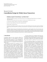
Figure 1: TSA airport tarmac surveillance dataset. Each image represents a block of 10 000 frames along with motion trajectories extracted.
200
150
100
50
50 100 150 200 250 300
(a)
200
150
100
50
50 100 150 200 250 300
(b)
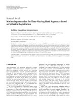
Figure 2: TSA airport tarmac surveillance dataset. Each image represents a block of 10 000 frames along with motion trajectories extracted.
algorithm is initialized with parameters learnt using training
data. If an unexpected state sequence is detected, an anomaly
is declared. This assumes that short-time dynamics is consis-
tent with the normal activity, but anomaly exists due to an
unexpected sequencing. Thus a completely unrelated activity
would not be declared an anomaly.
5. EXPERIMENTS

We demonstrate the usefulness of the online BMS model
for temporal segmentation and the offline BMS model for
anomaly detection using the following three datasets: the
TSA airport surveillance dataset, bank dataset, and the UCF
humanactiondataset.
5.1. TSA airport surveillance dataset
The TSA dataset consists of surveillance video captured at
an airport tarmac [2]. The stationary camera operates at
approximately 30 frames per second and the frame size is
320
× 240.
Though it is approximately 120 minutes long, a large
portion of the video does not contain any activities. We di-
vide the entire data into 23 blocks of about 10 000 frames
each. Here onwards, we refer to such sets of 10 000 frames
as blocks. Moving objects are detected and tracked as de-
scribed in Section 2.1. The background at each pixel was
modeled using a Gaussian distribution. The parameters are
reinitialized every hundred frames. Each frame is compared
with the background and the moving objects are detected. A
bounding box is drawn on the detected blobs. The KLT algo-
rithm is allowed to choose feature points for tracking within
the bounding box. The average trajector y of feature points
within the bounding box is regarded as the motion trajectory
of the objects (Figures 1 and 2). Since the video sequence is
long, it is impractical to obtain ground truth of t rajectories.
The activity model needs to be robust to imperfections in
tracking. The ground truth for temporal segmentation was
extracted manually, that is, by direct inspection of the video
sequences.

In four blocks, we observe a significant amount of mul-
tiobject activity when planes arrive and depart. The four
8 EURASIP Journal on Advances in Signal Processing
Table 1: TSA dataset: temporal segmentation of two blocks using
the online BMS model. GCP
= ground crew personnel, PAX = pas-
sengers, Det.
= segment detected, TF = tracking failed.
Number Block in Figure 1(a) Comment
1 2 GCP split, walk away Det.
2
GCP across tarmac Det.
3
Truck arrives, GCP Det.
4
GCP across tarmac Det.
5
Truck Det.
6
GCP movement Det.
7
Plane-I arrives Det.
8
Luggage cart to plane Det.
9
Truck crossing scene TF
Plane-II arrives Det.
10
GCP and lugg age cart —
approach plane-I Det.

11
— Extra segment
12
PAX disembark Det., 2 extra segments
Table 2: TSA dataset: temporal segmentation of two blocks using
the online BMS model. GCP
= ground crew personnel, PAX = pas-
sengers, Det.
= segment detected, TF = tracking failed.
Number Block in Figure 1(b) Comment
1 Luggage cart TF.
2
GCP movement near plane Det.
3
Luggage cart enter Det.
4
Plane enters Det.
5
PAX embark Det.
6
Luggage cart TF.
7
PAX embark Det.
blocks form the test set. Figures 1 and 2 show the motion
trajectories for these blocks. The remaining portion of the
dataset is used as the training set. It may seem large com-
pared to the size of the test set. The activity content, how-
ever, is not as dense as in the test set. The paucity of train-
ing data makes it unrealistic to train a model in the conven-
tional sense, where parameters of the mixed-state model are

estimated. Instead, we train an online BMS model, which in-
volves finding a basis of behavior. The values of parameters
are less important than the region of parameter space they
represent. Accordingly, the basis has elements that can pro-
duce the following types of motion: constant velocity along
a straight line, constant acceleration along a straight line,
curved trajectories with constant velocity, start, and stop.
We demonstrate temporal segmentation of the four test
blocks using the online BMS model. The segmentation re-
sults for the four blocks shown in Figures 1(a)-1(b) and 2(a)-
2(b) are summarized in Tables 1–4, respectively. On an aver-
age, there were 15% missed detections in segmentation. This
was mainly because of tracking errors.
Table 3: TSA dataset: temporal segmentation of two blocks using
the online BMS model. GCP
= ground crew personnel, PAX = pas-
sengers, Det.
= segment detected.
Number Block in Figure 2(a) Comment
1 Plane exits Det.
2
GCP movement Det.
3
Luggage cart to plane-II Det.
4
Bag falls off luggage cart Det.
5
Luggage cart to plane-II Det.
Table 4: TSA dataset: temporal segmentation of two blocks using
the online BMS model. GCP

= ground crew personnel, PAX = pas-
sengers, Det.
= segment detected, TF = tracking failed.
Number Block in Figure 2(b) Comment
1 2 GCP movement Det.
2
Luggage cart TF
3
GCP movement TF
4
Plane-II arrives Det.
5
GCP movement TF
6
Luggage cart to plane-II Det.
7
Plane-III arrives Det.
8
PAX embark Det.
9
Truck movement Det.
10
GCP near plane-II TF
11
Luggage cart from plane-II Det.
12
More P AX embark Det.
5.2. Bank surveillance dataset
The bank dataset consists of staged videos collected at a bank
[34]. There are four sequences, each approximately 15–20

seconds (∼400 frames) long. Figures 3 and 4 show sample
images from the dataset. The actors demonstrate two types
of scenarios.
(i) Attack scenario where a subject coming into the bank
forces his way into the restricted area. This is consid-
ered as an anomaly.
(ii) No attack scenario where subjects enter/exit the bank
and conduct normal transactions. This depicts a nor-
mal scenario. The normal process of transactions is
known a priori and we train an offline BMS model us-
ing these trajectories.
5.2.1. Temporal segmentation
We retained the same basis of behavior that was used for the
TSA dataset in Section 5.1. Though the TSA data is captured
outdoors and the bank data indoors, they are both surveil-
lance videos. They retain similarity at the primitive or behav-
ior level. For the no attack scenario, segmentation using the
online BMS model yielded two parts. In the first segment, we
see two subjects entering the bank successively. The first per-
son goes to the paper slips area and the second person goes to
N.P. Cuntoor and R. Chellappa 9
250
200
150
100
50
50 100 150 200 250 300 350
(a)
250
200

150
100
50
50 100 150 200 250 300 350
(b)
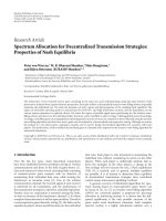
Figure 3: Bank dataset: two segments detected in the no attack scenario: (a) a subject enters the bank, goes to the area where paper slips are
stored. Another subject enters the bank and goes to the counter area, (b) exit bank.
250
200
150
100
50
50 100 150 200 250 300 350
(a)
250
200
150
100
50
50 100 150 200 250 300 350
(b)
250
200
150
100
50
50 100 150 200 250 300 350
(c)
0
5

10
15
20
0
5
10
15
20
Distance
0 100 200 300 400
Enter
bank
Go behind
counter
Exit
bank
84 242
(d)
Figure 4: Bank dataset: three segments detected in the attack scenario: (a) enter bank, (b) gain access to the restricted area behind the
counter, and (c) exit bank. (d) shows a plot of the switching function. Peaks in the plot indicate boundaries in temporal segmentation.
the counter. In the second segment, the two subjects leave the
bank. Figure 3 shows sample images from the two segments.
We store the parameters of these behavioral seg ments as the
normal activity.
Figure 4 shows an example of an attack scenario. Here,
the online BSM model yielded three segments. In the first
segment, the person enters the bank and proceeds to the area
where the deposit/withdrawal slips are kept. This is similar
to the first segment in the no attack case. During the second
segment, he follows another person into the restr icted area

behind the counter. The third segment consists of the person
leaving the bank.
10 EURASIP Journal on Advances in Signal Processing
Table 5: Compar ing no attack and attack scenarios in bank surveil-
lance data. L1 distance between histograms of parameters of online
BMS model is used as similarity score.
Number No attack Attack 1 Attack 2 Attack 3
No attack 0 310 424 362
Attack 1
310 0 218 278
Attack 2
424 218 0 180
Attack 3
362 278 180 0
5.2.2. Anomaly detection
The parameters of an offline BMS model are estimated using
the no attack scenario. To detect the presence of an anomaly,
we compute the error accumulated along the optimal state
sequence using the test trajectory. It is difficult to assess
the performance of this naive scheme since we have very
few samples. Alternatively, we use the online BMS model
to detect anomalies. If we assume that the attack scenarios
were normal activities while the no attack scenario was an
anomaly, we may expect the comparison scores of the dif-
ferent attack scenarios to be clustered together. For each of
the four scenarios in the dataset, parameters of their online
BMS models are computed. We form a similarity matrix of
size 4
× 4 in order to check whether the attack scenarios clus-
ter separately. The L1 distance between the histograms of pa-

rameters of learnt behavior is used as the similarity score.
Table 5 shows the distance between the different attack ex-
amples with the no attack case. We observe that the attack
scenarios are more similar to each other compared to the no
attack scenario.
5.2.3. Comparison of results
Georis et al. [34] presented an ontology-based approach for
video interpretation in which activities of interest are man-
ually encoded. They demonstrated the effectiveness of on-
tologies for detecting attacks on a safe in a bank monitoring
dataset. Their method requires a detailed description in the
form of a set of rules to detect an “attack” act ivity. The pro-
posed method, however, is data driven. The extent of devia-
tion observed in a given video sequence compared to a nor-
mal scenario is used as a measure for detecting anomalies.
Comparitive results are summarized below.
In [34], the authors repor t the following results on track-
ing persons in the bank scene: 88% true positives, 12% false
negatives, and 2% false positives. There were no errors in
tracking in our method.
For anomaly detection (i.e., detecting that the bank safe
was attacked), the results reported in [34]are93.5% of true
positives, 6.25% of false negatives, and 0% of false positives.
These results correspond to 16 repetitions of the attack sce-
nario. We have access to only 3 attack scenarios. On these, we
obtained correct anomaly detection in all three scenarios.
200
150
100
50

50 100 150 200 250 300
(a)
200
150
100
50
50 100 150 200 250 300
(b)
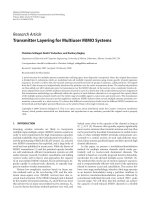
Figure 5: Sample images from UCF dataset.
5.3. UCF human action dataset
We may think of many actions as a sequence of behaviors.
For example, picking up an object may be abstracted as ex-
tend the hand toward object-grab object-withdraw the hand;
erasing the black board, as extend hand-move hand side to
side on the board-withdraw hand; opening the door, as ex-
tend hand-grab knob-withdraw hand. To generate an action,
we may compose a sequence of systems that operate with the
appropriate parameters.
The UCF database of human actions consists of 60 video
sequencescapturedinanoffice environment [13]. Examples
of actions include picking up an object, putting down an ob-
ject, opening the cabinet door, and pouring water into a cup.
A brief description of the low-level video processing algo-
rithms for extracting trajectories is given below. Further de-
tails are available in [13]. The dataset obtained from the UCF
group contains the extracted trajectories. The hand was de-
tected using a skin-detection algorithm. A mean-shift tracker
was initialized at the detected position to obtain motion tra-
jectory of the hand. The trajectories were smoothed out using
anisotropic diffusion. Figure 5 shows sample images from the

database along with extracted motion trajectories.
We employ the Viterbi-based segmentation described in
Section 4.1 to find the segments of actions. We show some
N.P. Cuntoor and R. Chellappa 11
100
150
200
250
30 50 70 90 110 130
(a)
110
130
150
170
190
40 80 120 160
(b)
80
120
160
200
240
50 70 90 110 130
(c)
80
120
160
200
240
20 60 100 140

(d)
120
140
160
180
200
20 60 100 140
(e)
80
120
160
200
240
20 60 100 140
(f)
100
140
180
220
260
50 70 90 110 130
(g)
190
210
230
250
270
0 40 80 120 160
(h)
110

130
150
170
190
20 40 60 80 100
(i)
70
90
110
130
10 30 50 70 90
(j)
80
120
160
200
240
40 60 80 100 120 140
(k)
170
190
210
230
250
50 70 90 110 130
(l)
120
160
200
240

280
100 120 140 160 180
(m)
80
120
160
200
240
110 130 150 170
(n)
100
140
180
220
260
300
80 120 160 200 240
(o)
Figure 6: Motion trajectories of the hand in the UCF dataset for different actions. The dots along the trajectory denote segment boundaries
detected.
of the segmentation results in Figure 6.Adescriptionofmo-
tion trajectories shown in Figure 6 along with the detected
segment boundaries is given below.
(a) Open cabinet door: start-reach door handle-open door-
w ithdraw hand.
(b) Pick up object: start-pick up object.
(c) Put down: start-putobjectincabinet-reachdoorhandle-
close door-withdraw hand .
(d) Open cabinet door: start-reach door handle-open door-
extra segment-withdraw hand.

(e) Pick up object: start-pick up object.
(f) Put down: start-putobjectincabinet-reachdoorhandle-
close door-withdraw hand .
(g) Open cabinet door: star t-reach door handle-open door-
w ithdraw hand.
(h), (i), (j) Pick up object: start-pick up object.
(k), (l) Open cabinet door: start-reach door handle-open
door-withdraw hand.
(m) Pick up and put down elsewhere: pick up-put down-
w ithdraw hand
(n) Open cabinet door (different viewing direction): start-
reach door handle-open door-withdraw hand.
(o) Pick up and put down elsewhere: pick up-put down
(late detection)-withdraw hand.
Table 6 shows the mean and variance of the number of seg-
ments detected for different activities. The same number of
segments were detected consistently across multiple samples
of activities picking up and pouring water an object. On the
other hand, variance in the number of segments detected
for picking up an object and putting it down elsewhere was
12 EURASIP Journal on Advances in Signal Processing
Table 6: Number of segments detected for activ ities in the UCF
indoor human action dataset.
Activity
Average no. of
Var ian ce
segments
Open door 4.44 0.53
Pick up 2.27 0.21
Put down 2.50 0.94

Close door 4.25 0.25
Erase 6.50 0.33
Pour water 3.00 0.00
Pick up object and
put down elsewhere
3.75 3.92
high. This was because of excessive differences in appearance
across samples.
5.3.1. Comparison of results
We compared the location of detected segment boundaries
with the dynamic instants described in [13]. Dynamic in-
stants are points of high curvature along the trajectory. They
are chosen as the feature of interest to ensure view invari-
ant representation of actions. The first segm ent switching
in the proposed approach occurs after sufficient evidence
about the dynamics has been accumulated. This is marked
as the start segment, which usually occurs in 10–15 frames.
We ignore this boundary point when comparing our results
with dynamic instants in [13] since it does not have an ex-
plicit start instant. Segment boundaries detected using our
method, which are marked by dots in Figure 6 are compared
with the dynamic instants in [13]. The average difference
between the two values are as follows: 5.4framesforopen
door, 4.1framesforclosedoor,3.3framesforpourwater,2.0
frames for erase board, and 6.2 frames for pick up object and
put down elsewhere.
5.4. Homecare applications
Though the proposed approach was demonstrated using
video sequences collected in office and airport environments,
it can be easily applied to home-care scenarios. DeNatale et

al. [35] describe fall detection and accessing unauthorized
locations as typical applications in home-care scenarios. We
highlight the applicability of our method to some home-care
applications.
As demonstrated using the bank monitoring dataset, our
approach is able to detect if a person gained access to unau-
thorized places. Similarly, as experiments using the UCF
dataset demonstrated, human actions were segmented into a
sequence of elementary parts. For instance, opening a cabinet
door was represented as start-reach door handle-open door-
w ithdraw hand. These actions could be used to find the num-
ber of times medicine cabinet is used. If an opening action
does not occur at expected times, an alarm could be issued.
6. SUMMARY
It is important to build activity models that generalize across
scenarios so that they enhance portability and adaptability.
Even within a scenario, it may not be realistic to enumerate
all possible activities during the design process. Instead, the
system should be capable of learning new behavioral mod-
els. Approaches that are completely data driven may not be
ideal since combinatorially many alternatives have to be con-
sidered.
To summarize, we have described piecewise linear mixed-
state models for representing activities using motion trajec-
tories as observed data. A sequence of such segments is said
to characterize an activity based on a context-independent
basis of behavior. Parameters of the segmentwise models
and switching times between them were estimated using
a Viterbi-based algorithm. Experiments using surveillance
video streams in both indoor and outdoor settings demon-

strate that the method can be used to analyze activities at
different scales. The usefulness of the proposed method is
shown using applications such as temporal segmentation
and anomaly detection. As part of future work, we will in-
vestigate ways to learn the basis elements from training se-
quences.
APPENDIX
BAUM-WELCH ALGORITHM
This section contains a brief overview of the Baum-Welch
algorithm that was introduced in [31]. There are several
sources that offer a detailed explanation (e.g., [29, 31]). Let
λ
= (A, B, Π) represent an HMM, where A = [a
ij
] is the
transition probability matri x, B contains emission probabili-
ties conditioned on the current state, and Π is the initial dis-
tribution of states. Let O
={o
1
, o
2
, , o
T
} be the observa-
tion sequence. The Baum-Welch algorithm is an expectation-
maximization (EM) algorithm that can compute parameters
of A, B,andΠ such that the likelihood function P(O
| λ)is
maximized. It involves the following steps.

(i) Choose the initial parameters of λ (usually through a
k-means procedure).
(ii) Reestimate the parameters using the forward and
backward variables. This is equivalent to computing
estimates such that
a
ij
=
expected no. of transitions from state i to j
expected no. of t ransitions from state i
,
b
j
(o) =
expected no. of times in statej and observing o
expected no. of times in state j
.
(A.1)
(iii) Iterate until convergence.
N.P. Cuntoor and R. Chellappa 13
ACKNOWLEDGMENT
This work was partially supported by the ARDA/VACE Pro-
gram under the Contract 2004H80200000.
REFERENCES
[1] B. Sin and J. H. Kim, “Nonstationary hidden Markov model,”
Signal Processing, vol. 46, no. 1, pp. 31–46, 1995.
[2] N. Vaswani, A. R. Chowdhury, and R. Chellappa, “Activity
recognition using the dynamics of the configuration of inter-
acting objects,” in Proceedings of the IEEE Computer Society
Conference on Computer Vision and Pattern Recognition (CVPR

’03), vol. 2, pp. 633–640, Madison, Wis, USA, June 2003.
[3] J. K. Aggarwal and Q. Cai, “Human motion analysis: a review,”
Computer Vision and Image Understanding,vol.73,no.3,pp.
428–440, 1999.
[4] T. Starner and A. Pentland, “Real-time American Sign Lan-
guage recognition from video using hidden Markov models,”
in Proceedings of the IEEE International Symposium on Com-
puter Vision (ISCV ’95), pp. 265–270, Coral Gables, Fla, USA,
November 1995.
[5] R. Polana and R. Nelson, “Low level recognition of human
motion (or how to get your man without finding his body
parts),” in Proceedings of the IEEE Workshop on Motion of Non-
Rigid and Articulated Objects, pp. 77–82, Austin, Tex, USA,
November 1994.
[6] A. Bobick and J. Davis, “Real-time recognition of activity us-
ing temporal templates,” in Proceedings of the 3rd IEEE Work-
shop on Applications of Computer Vision (WACV ’96), pp. 39–
42, Sarasota, Fla, USA, December 1996.
[7] Y. A. Ivanov and A. F. Bobick, “Recognition of visual activities
and interactions by stochastic parsing,” IEEE Transactions on
Pattern Analysis and Machine Intelligence, vol. 22, no. 8, pp.
852–872, 2000.
[8] A. Kale, A. Sundaresan, A. N. Rajagopalan, et al., “Identifica-
tion of humans using gait,” IEEE Transactions on Image Pro-
cessing, vol. 13, no. 9, pp. 1163–1173, 2004.
[9] T. Izo and W. E. L. Grimson, “Simultaneous pose estimation
and camera calibration from multiple views,” in Proceedings of
IEEE Workshop on Motion of Non-Rigid and Articulated Ob-
jects, vol. 1, pp. 14–21, Washington, DC, USA, June 2004.
[10] M. Brand, N. Oliver, and A. Pentland, “Coupled hidden

Markov models for complex action recognition,” in Proceed-
ings of the IEEE Computer Society Conference on Computer Vi-
sion and Pattern Recognition (CVPR ’97), pp. 994–999, San
Juan, Puerto Rico, USA, June 1997.
[11] R. Nevatia, T. Zhao, and S. Hongeng, “Hierarchical language-
based representation of events in video streams,” in Proceed-
ings of 2nd IEEE Workshop on Event Mining: Detection and
Recognition of Events in Video, vol. 4, pp. 39–45, Madison, Wis,
USA, June 2003.
[12] T. Syeda-Mahmood, A. Vasilescu, and S. Sethi, “Recogniz-
ing action events from multiple viewpoints,” in Proceedings of
IEEE Workshop on Detection and Recognition of Events in Video,
Vancouver, Canada, July 2001.
[13] C. Rao, A. Yilmaz, and M. Shah, “View-invariant representa-
tion and recognition of actions,” International Journal of Com-
puter Vision, vol. 50, no. 2, pp. 203–226, 2002.
[14] D. Koller and U. Lerner, “Sampling in factored dynamic sys-
tems,” in Sequential Monte Carlo Methods in Practice, pp. 445–
464, Springer, New York, NY, USA, 2001.
[15] R. Hamid, Y. Huang, and I. Essa, “ARGMode—activity recog-
nition using graphical models,” in Proceedings of IEEE Com-
puter Society Conference on Computer Vision and Pattern
Recognition (CVPR ’03), vol. 4, pp. 38–43, Madison, Wis, USA,
June 2003.
[16] V. Vu, F. Bremond, and M. Thonnat, “Automatic video inter-
pretation: a novel algorithm for temporal scenario recogni-
tion,” in Proceedings of the 18th International Joint Conferences
on Artificial Intelligence (IJCAI ’03), Acapulco, Mexico, August
2003.
[17] M. Isard and A. Blake, “A mixed-state condensation tracker

with automatic model-switching,” in Proceedings of the 6th
IEEE International Conference on Computer Vision (ICCV ’98),
pp. 107–112, Bombay, India, January 1998.
[18] Z. Ghahramani and G. E. Hinton, “Variational learning for
switching state-space models,” Neural Computation, vol. 12,
no. 4, pp. 831–864, 2000.
[19] A. B. Kurzhanski and P. Varaiya, “Dynamic optimization for
reachability problems,” Journal of Optimization Theory and
Applications, vol. 108, no. 2, pp. 227–251, 2001.
[20] C. Tomlin, G. J. Pappas, and S. Sastr y, “Conflict resolution
for air traffic management: a study in multiagent hybrid sys-
tems,” IEEE Transactions on Automatic Control,vol.43,no.4,
pp. 509–521, 1998.
[21] C. Stauffer and W. E. L. Grimson, “Learning patterns of ac-
tivity using real-time tracking,” IEEE Transactions on Pattern
Analysis and Machine Intelligence, vol. 22, no. 8, pp. 747–757,
2000.
[22] V. Parameswaran and R. Chellappa, “View invariance for hu-
man action recognition,” International Journal of Computer Vi-
sion, vol. 66, no. 1, pp. 83–101, 2006.
[23] D. G. Kendall, D. Barden, T. K. Carne, and H. Le, Sh ape and
Shape Theory, John Wiley & Sons, New York, NY, USA, 1999.
[24] H. Zhong, J. Shi, and M. Visontai, “Detecting unusual activity
in video,” in Proceedings of the IEEE Computer Society Confer-
ence on Computer Vision and Pattern Recognition (CVPR ’04),
vol. 2, pp. 819–826, Washington, DC, USA, June 2004.
[25] I. Haritaoglu, R. Cutler, D. Harwood, and L. S. Davis, “Back-
pack: detection of people carrying objects using silhouettes,”
in Proceedings of the 7th IEEE International Conference on
Computer Vision (ICCV ’99), vol. 1, pp. 102–107, Kerkyra,

Greece, September 1999.
[26] C. R. Wren, A. Azarbayejani, T. Darrell, and A. P. Pentland,
“Pfinder: real-time tracking of the human body,” IEEE Trans-
actions on Pattern Analysis and Machine Intelligence, vol. 19,
no. 7, pp. 780–785, 1997.
[27] B. D. Lucas and T. Kanade, “An iterative image registration
technique with an application to stereo vision,” in Proceed-
ings of the 7th International Joint Conference on Artificial Intel-
ligence (IJCAI ’81) , pp. 674–679, Vancouver, BC, Canada, Au-
gust 1981.
[28] Y. Ephraim, A. Dembo, and L. R. Rabiner, “Minimum discrim-
ination information approach for hidden Markov modeling,”
IEEE Transactions on Information Theory,vol.35,no.5,pp.
1001–1013, 1989.
[29] L. R. Rabiner, “A tutorial on hidden Markov models and se-
lected applications in speech recognition,” Proceedings of the
IEEE, vol. 77, no. 2, pp. 257–286, 1989.
[30] M. Vidyasagar, Nonlinear Systems Analysis, Prentice Hall, En-
glewood Cliffs, NJ, USA, 1993.
[31] L. Baum, T. Petrie, G. Soules, and N. Weiss, “A maximiza-
tion technique occuring in the statistical analysis of probabilis-
tic functions of Markov chains,” The Annals of Mathematical
Statistics, vol. 41, no. 1, pp. 164–171, 1970.
14 EURASIP Journal on Advances in Signal Processing
[32] G. D. Forney Jr., “The Viterbi algorithm,” Proceedings of the
IEEE, vol. 61, no. 3, pp. 268–278, 1973.
[33] A. Kav
ˇ
ci
´

c and J. M. F. Moura, “The Viterbi algorithm and
Markov noise memory,” IEEE Transactions on Information
Theory, vol. 46, no. 1, pp. 291–301, 2000.
[34] B. Georis, M. Maziere, F. Bremond, and M. Thonnat, “A video
interpretation platform applied to bank agency monitoring,”
in Proceedings of Workshop on Intelligent Distributed Surveil-
lance Systems (IDSS ’04), pp. 46–50, London, UK, February
2004.
[35] F.DeNatale,O.Mayora-Ibarra,andL.Prisciandaro,“Interac-
tive home assistant for supporting elderly citizens,” in Proceed-
ings of EUSAI Workshop on Ambient Intelligence Technologies
for WellBeing at Home, Eindhoven, The Netherlands, Novem-
ber 2004.
Naresh P. Cuntoor received the B .E. de-
gree in electronics and communication en-
gineering from the Karnataka Regional En-
gineering College (now renamed National
Institute of Technology), Surathkal, India,
in 2000, and the M.S. degree in electrical
and computer engineering from the Uni-
versity of Maryland, College Park, in 2003,
where he is currently pursuing the Ph.D. de-
gree in electrical and computer eng ineering.
His research interests include computer vision, statistical pattern
recognition, image processing, differential geometry, and topology.
Rama Chellappa received the B.E.(Hons)
degree from the University of Madras, In-
dia, in 1975, and the M.E.(Distinction)
degree from the Indian Institute of Sci-
ence, Bangalore, in 1977. He received the

M.S.E.E. and Ph.D. degrees in electrical
engineering from Purdue University, West
Lafayette, IN, in 1978 and 1981, respec-
tively. Since 1991, he has been a Professor of
electrical engineering and an Affiliate Pro-
fessor of Computer Science at the University of Maryland, College
Park. Recently, he was named the Minta Martin Professor of En-
gineering. He is also affiliated with the Center for Automation Re-
search (Director) and the Institute for Advanced Computer Studies
(PermanentMember). Prior to joining the University of Maryland,
he was an Assistant Professor (1981–1986) and an Associate Profes-
sor (1986–1991) and Director of the Signal and Image Processing
Institute (1988 to 1990) with the University of Southern California
(USC), Los Angeles. Over the last 25 years, he has published nu-
merous book chapters and peer-reviewed journal and conference
papers. He has also coedited and coauthored many research mono-
graphs. His current research interests are face and gait analysis, 3D
modeling from video, automatic target recognition from stationary
andmoving platforms, surveillance and monitoring, hyperspectral
processing, image understanding, and commercial applications of
image processing and understanding.