Báo cáo hóa học: " Research Article Synthetic Stimuli for the Steady-State Verification of Modulation-Based Noise Reduction Systems" docx

Hindawi Publishing Corporation
EURASIP Journal on Advances in Signal Processing
Volume 2009, Article ID 876371, 8 pages
doi:10.1155/2009/876371
Research Article
Synthetic Stimuli for the Steady-State Verification of
Modulation-Based Noise Reduction Systems
Jesko G. Lamm (EURASIP Member), Anna K. B erg, and Christian G. Gl
¨
uck
Bernafon AG, Morgenstrasse 131, 3018 Bern, Switzerland
Correspondence should be addressed to Jesko G. Lamm,
Received 28 November 2008; Accepted 12 March 2009
Recommended by Heinz G. Goeckler
Hearing instrument verification involves measuring the performance of noise reduction systems. Synthetic stimuli are proposed
as test signals, because they can be tailored to the parameter space of the noise reduction system under test. The article presents
stimuli targeted at steady-state measurements in modulation-based noise reduction systems. It shows possible applications of these
stimuli and measurement results obtained with an exemplary hearing instrument.
Copyright © 2009 Jesko G. Lamm et al. This is an open access article distributed under the Creative Commons Attribution License,
which permits unrestricted use, distribution, and reproduction in any medium, provided the original work is properly cited.
1. Introduction
Noise reduction systems provide users of hearing instru-
ments with increased listening comfort [1]. The aim of such
systems is to suppress uncomfortable sounds on the one
hand, but to preserve speech on the other hand. Among
various available noise reduction methods, modulation-
based processing is a common one [2].
Modulation-based noise reduction systems apply differ-
ent amounts of attenuation in different frequency ranges,
depending on the likelihood of speech presence in each of
them. Based on the observation that speech has a char-

acteristic modulation spectrum [3], such systems measure
modulation, which is the fluctuation of the signal’s envelope
over time.
The measurements treat modulation in different sub-
bands separately, such that the signal processing can react
by applying different amounts of attenuation in different
frequency ranges. The idea is to attenuate signals that lack
the characteristic modulation of speech.
Testing a hearing instrument regarding noise reduction
performance has to ensure that two conditions are met.
(i) The noise reduction system meets its requirements.
(ii) The noise reduction system satisfies its user.
Assessing each of these conditions requires an individual
test philosophy: while verification shows if the noise reduc-
tion system meets its requirements, validation assesses the
system’s capability of meeting customer needs “in the most
realistic environment achievable” [4].
In the following, we present a measurement-based test
procedure for modulation-based noise reduction systems in
hearing instruments. Our focus is on verification and not on
validation, because the validation of noise reduction systems
in hearing instruments has been discussed well in literature
(e.g., [5]).
Numerous stimulus-based verification procedures for
different aspects of hearing instrument functionality have
been presented so far. Here are two recent examples.
(i) The International Speech Test Signal [6, 7]isa
stimulus for measuring the hearing instrument per-
formance in a speech-like environment. It is based
on a combination of numerous real-world speech

signals.
(ii) Bentler and Chiou have discussed the verification of
noise reduction systems in hearing instruments and
presented measurements based on real-world speech
in noise [8].
The above examples are both based on real-world speech
signals. This makes sense, because suitable performance in
speech is essential for hearing instruments. In this article,
however, noise plays an important role, because noise is the
reason why noise reduction systems are needed.
Real-world noise signals lack certain properties desirable
in test signal design. These properties are mainly [9–11]
2 EURASIP Journal on Advances in Signal Processing
(i) the possibility of configuring certain signal character-
istics (like, e.g., modulation) systematically in order
to force the system under test into a desired state;
(ii) freedom in changing the signal’s temporal charac-
teristics, selecting its power-spectrum, and making
its spectral components sufficiently constant over the
frequency range of interest.
We have therefore recently proposed synthetic test signals
[9], because these can be synthesized with regard to the
temporal characteristics of interest, the systematic estimation
of noise reduction parameters, and accurate measurement
results.
Using synthetic test signals in the audio processing
domain is not new. In telephony applications, a so-called
Composite Source signal [12] based on synthetic speech is
available for verification of transfer characteristics of tele-
phony equipment. In that case, again the speech performance

of the system under test is of major interest, whereas the noise
reduction stimuli which we describe in the following mainly
focus on noise attenuation by the noise reduction system
under test.
This article shows some new results and applications
with the synthetic test signals from [9] in measuring the
noise reduction attenuation in dependency of different input
parameters. We first summarize and explain the signal
synthesis procedure from [9]. Then we show different
applications of the synthetic test signals. These are finally
illustrated with measurement results, which we obtained
with an exemplary hearing instrument.
2. Synthetic Test Stimuli
2.1. Requirements Towards the Stimuli. A noise reduction
system should attenuate noise, which makes the attenuation
a parameter of major interest in testing. Since a typical
noise reduction system operates in multiple subbands [1],
a systematic test procedure should measure the attenuation
in each of them separately. It is therefore required that
the test stimuli can stimulate each subband of the noise
reduction individually and measure the impact on the
system’s frequency response.
As a consequence, the stimuli have to meet the following
demands: they should not only perform well in frequency
response measurements, but they should also allow signal
parameters to be set individually for different frequency
ranges. For example, the stimuli for verifying modulation-
based noise reduction should have a constant magnitude in
the frequency range of interest (see [11]) and furthermore
different well-defined modulation depths in different fre-

quency ranges.
The peak factor [13] of the signals should be as low as
possible, because a high peak factor implies that a signal of
given power has high amplitude peaks, resulting in distortion
by nonlinearities not only in the measurement equipment
but also in the hearing instrument under test itself.
The signals should also be periodic, since periodicity
brings the following advantages.
(i) Periodic stimuli avoid leakage errors [14] in process-
ing based on Discrete Fourier Transforms (DFT).
(ii) Measuring the magnitude of a system’s frequency
response becomes independent of the system’s
throughput delay when using a periodic stimulus,
becausewithinagiventimeframewhoselengthisan
integer number of periods, the throughput delay of
the system only produces a phase shift and thus has
no impact on the measured magnitude.
(iii) Only one period of the desired stimulus needs to be
computed, which limits synthesis time.
(iv) The stimulus can be described by means of its
complex Fourier coefficients c
k
via complex Fourier
series. If the stimulus is σ,itsperiodisT,andj is
the imaginary unit, then the Fourier Series repre-
sentation of the stimulus is given by the following
equation:
σ
(
t

)
=
∞

k=−∞
c
k
·e
j 2π (kt/T)
. (1)
Note that a disadvantage of a periodic signal is its
discrete power-spectrum: measuring frequency responses
with periodic stimuli will only cover discrete frequencies. See,
for example, [14] for nonperiodic alternatives.
2.2. Signal Synthesis
2.2.1. Simple Subband Signals Based on Sinusoids. The most
trivial subband signal is a sine wave. Rated against the
requirements from Section 2.1,asinewaveperformswell
regarding peak factor and periodicity, but does not have the
required constant magnitude over the frequency range of
interest. This can be addressed in using multiple sines: a
test stimulus obtained by summing sine waves of different
frequencies will indeed cover a certain frequency range;
however, summing sine waves requires special care, as will
be explained below.
We call a sum of sine signals a multisine. Summing sine
signals with carelessly chosen phase angles typically yields
a multisine with a high peak factor [13] as opposed to the
lowpeakfactorrequiredinSection 2.1. By choosing the
right phase angles, the peak factor can be reduced: there are

various algorithms for determining combinations of phase
angles that yield a low peak factor in summing sine waves
[13–16].
An exemplary multisine synthesis algorithm [15]has
recently been evaluated in synthesizing stimuli for the
verification of a noise reduction system in an exemplary
hearing instrument [9]. Some poor results during this
evaluation made us focus on noise-based stimuli, which will
be discussed in the following. Note that it is still an open
question whether multisines are a suitable basis for noise
reduction stimuli, but we would like to exclude that question
from this article’s scope.
EURASIP Journal on Advances in Signal Processing 3
−1.5
0
1.5
Amplitude
1024 2048 3072 4096
Sample number
Original signal (peak factor: 3.5)
(a)
−0.5
0
0.5
Amplitude
1024 2048 3072 4096
Sample number
Filtered signal (peak factor: 6.3)
(b)
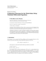
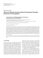
Figure 1: A noise signal (a) and the result of filtering it through

a bandpass filter whose passband corresponds to a typical noise
reduction subband (b).
2.2.2. Simple Subband Signals Based on Noise. A simple way
of synthesizing a band-limited noise signal in the frequency
range of a noise reduction subband is
(i) generating a noise signal,
(ii) filtering the noise signal with a bandpass filter
whose pass-band corresponds to the noise reduction
subband of interest.
Figure 1 shows an example: MATLAB’s “rand” function
was used to generate a uniformly distributed digital noise
signal (Figure 1(a)). This signal was filtered with a bandpass
filter corresponding to a typical noise reduction subband
(Figure 1(b)).
However, the example in Figure 1 illustrates two reasons
for why bandpass-filtering a noise signal will in general
not produce a stimulus that meets the requirements from
Section 2.1as follows.
(i) The stimulus has a high peak factor (e.g., a peak
factor of 6.3 in the case of the signal shown in
Figure 1(b)).
(ii) It is not possible to determine the modulation
depth of the stimulus (see, e.g., the signal shown in
Figure 1(b), which has some fluctuations in its enve-
lope although it has not explicitly been modulated).
Obviously, subband signals that have been obtained by
filtering a broadband signal are not well-suited as noise
reduction stimuli. Therefore we propose to choose a synthe-
sis procedure capable of constructing band-limited signals
that have a low peak factor.

2.2.3. Band-Limited Discrete-Interval Binary Sequences. A
signal whose amplitude has only two discrete values is called
a binary signal. Obviously, binary signals have a minimum
peak factor and therefore perfectly satisfy the peak factor
requirement from Section 2.1. However, binary signals also
tend to have a wide bandwidth, which disqualifies most of
them from subband measurements.
The theory of discrete-interval binary signals [17, 18]pro-
vides algorithms that search binary signals with amplitude
changes at multiples of a certain time interval for those
signals whose power spectrum approximates a desired one.
This theory can be used here to find binary signals whose
power is concentrated in one subband and whose power
spectrum is sufficiently constant for frequency response
measurements.
Although binary signals have a minimum peak factor, it
is not a necessary property for a noise reduction stimulus
to be binary. We expect various kinds of signals to be
suitable stimuli, like, for example, the multisines mentioned
in Section 2.2.1. For our further considerations, however, we
limit our scope to discrete-interval binary signals, because
these performed well in our evaluation of different stimuli,
as shown exemplarily in [9]. Since signal synthesis should
work in discrete-time and discrete-interval binary signals
were originally defined in continuous time [17], we define
that a discrete-interval binary sequence is the discrete-time
representation of a discrete-interval binary signal.
The Frequency Domain Identification Toolbox (FDI-
DENT) for MATLAB [19]offers readily accessible functions
for synthesizing discrete-interval binary sequences [16]. The

“dibs” function in this toolbox takes absolute values of
desired Fourier coefficients as an input and returns one
period of a periodic discrete-interval binary sequence whose
Fourier series approximates the given input.
When used as a stimulus for subband measurements,
a periodic discrete-interval binary sequence needs to have
its power concentrated in the frequency range of inter-
est, ideally like band-limited white noise. Therefore, if
the frequency range of interest is from f
1
to f
2
(where
f
1
> 0andf
2
≥ f
1
+ T
−1
) and the desired RMS of
the synthesized signal is r, then the target values for the
synthesis algorithm are given by the following absolute values
of Fourier coefficients c
k
(derived from [9]):


c

k


=
⎧
⎪
⎪
⎨
⎪
⎪
⎩
r

2


T·f
2

−

T·f
1

+1

;

T·f
1


≤|
k|≤

T·f
2

0 else.
(2)
3. Frequency Response Measurements
3.1. General Procedure. Inthissection,wedescribeaproce-
dure for stimulus-based measurements of a linear system’s
frequency response. It is based on digital signal processing
and thus assumes that test stimuli and the output signal
of the system under test are available as digital waveforms.
All further considerations will be made with regard to the
following measurement procedure.
DFT-based processing can approximate the frequency
response function of a system whose input stimulus is a
periodic digital test signal: the system’s output is digitized
4 EURASIP Journal on Advances in Signal Processing
with the clock of the input signal. Then, the DFT is applied to
both the input signal and the digitized output. The frequency
response is calculated at each DFT frequency by dividing
the absolute value of the output-related DFT bin by the
corresponding input-related value [11, 20]. Leakage errors
can be avoided if the stimulus is periodic, and if the DFT
window contains an integer number of its periods [14].
The described procedure requires a steady-state condi-
tion of the system under test. Therefore all measurements

described here are steady-state measurements.
3.2. Subband Measurements with Narrow-Band Stimuli. A
very simple test case is the measurement of the frequency
response in one noise reduction subband. Let the number
of subbands be M. We assign an index i
∈{1, 2, 3, , M}
to each of them. Let the lower and upper band limit of band
number i be f
c,i
and f
c,i+1
, respectively. Furthermore, let u
i
be
a discrete-interval binary sequence that has been synthesized
according to a target by (2), where f
1
= f
c,i
,and f
2
= f
c,i+1
.
We can now construct a signal with modulation fre-
quency f
m,i
and a configurable modulation depth: let m
i
be another discrete-interval binary sequence that has been

synthesized in the same way as u
i
,butwithf
1
= f
c,i
+ f
m,i
and
f
2
= f
c,i+1
− f
m,i
, where the modification of the band limits
by
±f
m,i
should compensate for the broadened spectrum
that results when modulating m
i
with modulation frequency
f
m,i
. Note that m
i
and u
i
are completely unmodulated. Now

a signal s
i
of modulation frequency f
m,i
and configurable
modulation depth is given by
s
i
(
t
)
= α ·

2
3
·m
i
(
t
)
·

1+cos

2πf
m,i
t

+
(

1 −α
)
·u
i
(
t
)
.
(3)
In (3), parameter α
∈ [0, 1] configures the modulation
depth. The factor
√
2/3 ensures that the s
i
signals resulting
from α
= 0andα = 1 have approximately the same
RMS, such that the signal power of s
i
is almost independent
of the modulation depth configured by parameter α.In
theory, the approximative factor
√
2/3couldbereplacedby
the precise factor that is needed to make the signal power
completely independent from α. This precise factor could be
computed from the known signals m
i
and u

i
.However,in
the applications we present here, this is in our opinion not
necessary: in the examples we show in this article based on
the approximative factor
√
2/3, we computed the signal level
of s
i
for the cases α = 0andα = 1 and found that it differs by
less than 0.05 dB from one case to the other.
Note that the stimuli we present here are defined in con-
tinuous time, but targeted at a measurement procedure using
discrete-time processing. The link between the continuous-
time domain and the discrete-time domain is in our case
given by the earlier-mentioned FDIDENT toolbox: It takes
Fourier coefficients from the continuous-time domain as
an input and returns a discrete-interval binary sequence as
discrete-time signal. Therefore, the following discrete-time
version of (3) is needed (where n is the sample index, f
s
is
the sampling frequency and
m
i
, u
i
, s
i
are the discrete-time

signals resulting from sampling m
i
, u
i
,ands
i
,resp.):
s
i
(
n
)
= α ·

2
3
· m
i
(
n
)
·

1+cos

2π
f
m,i
f
s

n

+
(
1 −α
)
· u
i
(
n
)
.
(4)
The signal from (4) can be used for measuring the
frequency response of a hearing instrument in the subband of
interest with the procedure from Section 3.1. The frequency
response of the noise reduction system in the hearing
instrument can be obtained by a differential measurement;
this means that the frequency response is first measured
with the noise reduction turned on and then with the noise
reduction switched off. Frequency-by-frequency division of
the obtained responses yields the transfer function of the
noise reduction.
Note that the signal presented in this section is only
targeted at a single subband. Therefore all measurement
samples at frequencies outside the given subband have to be
ignored. The next section describes stimuli that measure the
frequency response of the noise reduction system over the
whole bandwidth of the hearing instrument.
3.3. Full Bandwidth Measurements with Broadband Stimuli.

This section describes the synthesis of a signal that allows
measuring the frequency response over the whole bandwidth
of the hearing instrument under test. The idea is to measure
the effect of the noise reduction system in a certain subband,
while the noise reduction does not act on any other frequency
range. Let the subband of interest be b. To obtain a test signal
θ
b
that evokes attenuation of a modulation-based noise
reduction system in subband number b only, we add a signal
that is designed with configurable modulation and limited to
have most of the signal power in subband number b to fully
modulated signals corresponding to the other subbands:
θ
b
(
n
)
= s
b
(
n
)
+

2
3
·

i∈

(
{1,2, ,M}\{b}
)
m
i
(
n
)
·

1+cos

2π
f
m,i
f
s
n

.
(5)
Here again, M is the number of subbands. The signal
s
b
in (5) is the same as in (4). This means that the modulation
depth of signal
s
b
can be configured via parameter α
according to (4).

Note the following: if the value of α is close to 1, some
segments of signal
s
b
are close to zero (those segments in
which the cosine in (4) is close to
−1). As the m
i
signals
in (5) are discrete-interval binary sequences, they will not
be perfectly band-limited and therefore produce side-lobes
in subband number b. This means that the stimulus in the
subband of interest is infringed by sidelobes from other
bands for values of α close to 1.
As a consequence, the test signal θ
b
from (5)isnot
well-suited for measuring noise reduction performance as a
function of modulation depth parameter α in its full range.
EURASIP Journal on Advances in Signal Processing 5
However, for α
= 0, signal θ
b
can be used for measuring the
frequency response of the noise reduction system while one
subband is stimulated to apply its maximum attenuation. We
show an example of this application in Section 5.4.1.
3.4. Subband Measurements with Broadband Stimuli. So far
we have presented the synthesis of noise reduction stimuli
for different subbands and a way of mixing these stimuli in

order to obtain a test signal θ
b
for broadband measurements.
We argued that test signal θ
b
causes problems with high
modulation depths due to side-lobe influences from other
subbands. In this section we show a way of eliminating these
side-lobe influences in one subband of interest.
If subband number b is the subband of interest, then
we can eliminate the influences from other subbands by
filtering out their side lobes from this particular subband.
This can be done using a band-stop filter whose band limits
are the crossover frequencies of subband number b.Leth
be the impulse response of such a band-stop filter, and let
“
∗” be the convolution operator. Furthermore let

θ
b
be a
modified version of θ
b
in which side-lobe influences from
other subbands will be eliminated. We construct

θ
b
by a
modified version of (5)


θ
b
(
n
)
= s
b
(
n
)
+

2
3
·h
(
n
)
∗

i∈
(
{1,2, ,M}\{b}
)
m
i
(
n
)

·

1+cos

2π
f
m,i
f
s
n

.
(6)
In practice, we do not implement the band-stop filter by a
convolution with h. We rather implement the filtering in the
DFT domain: we put zeros into the stop-band’s DFT bins of
the signal to filter, exploiting the periodicity of the
m
i
signals
and of the cosine term in (6).
Note that

θ
b
can have a higher peak factor than θ
b
due to the filtering. In the measurements we describe in
Section 5.4.2, this was however not a problem. If only one
subband of interest is within the scope of the test, then the

narrow-band stimuli from Section 3.2 can be used. The test
signal

θ
b
is useful when all subbands of the noise reduction
system are relevant in the test case, but modulation will only
be varied in one of them.
4. Attenuation Function Measurements
Modulation-based noise reduction systems apply attenua-
tion as a function of the signal’s modulation depth [8].
Therefore, the dependency between modulation depth and
attenuation is of interest in noise reduction testing. For sys-
tems that operate in multiple subbands, this dependency can
be assessed per subband, if varying modulation parameter α
according to (4) and then using each resulting signal
s
i
either
as a stimulus for measurement or as a basis for synthesizing
stimulus

θ
b
according to (6).
The resulting stimuli can be used in measuring the
frequency response of a subband of interest for different
modulation depths. In order to obtain a simple modula-
tion/attenuation dependency function, one needs to com-
pute a single attenuation value from a transfer function

defining gain at multiple frequencies. Inspired by the way
in which median and averaging operations work, we here
propose sorting a certain set of gain values within the
subband of interest by their magnitude and then averaging
those values that remain after eliminating the first and the
last quarter of the resulting sorted list. Typically, one would
only choose frequencies close to the center frequency of the
current subband in order to avoid taking the slopes at the
band limits into the averaging process.
5. Examples
5.1. System under Test. An exemplary digital hearing instru-
ment with a modulation-based noise reduction system was
the system under test for the measurements whose results are
presented further below. The noise reduction system in this
hearing instrument works in the time domain according to
the following scheme.
(i) Determine the amount of typical modulation in
different subbands of the hearing instrument’s input
signal by passing subband signals through running
maximum and minimum filters and comparing the
different filters’ outputs [1].
(ii) For each subband, compute attenuation as a function
of modulation, where low modulation maps to high
attenuation and vice versa.
(iii) Use a controllable filter to adjust the frequency
response of the hearing instrument as it is given
by the computed frequency-dependent attenuation
values.
More details on the underlying concept of implementing
modulation-based noise reduction in the time domain can

be found in [1].
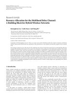
5.2. Measurement Setup. A test system was set up for making
measurements with synthetic test signals. Figure 2 illustrates
the setup: the hearing instrument under test is located in an
off-the-shelf acoustic measurement box with a loudspeaker
(L
1
) for presenting test stimuli to be picked up by the
hearing instrument’s input transducer (M
2
). The hearing
instrument’s output transducer (L
2
) is coupled with a
measurement microphone (M
1
) so tightly that environment
sounds can be neglected in comparison to the hearing
instrument’s output. The coupler is a cavity that is similar to
the human ear canal. Here, we used a so-called 2cc-coupler.
A digital playback and recording system can play
MATLAB-created stimuli via a digital-to-analogue converter
(D/A) and the loudspeaker of the measurement box (L
1
),
while recording the hearing instrument’s output via the mea-
surement microphone and an analogue-to-digital converter
(A/D). The recorded digital data is stored in a MATLAB-
readable file on a hard disk. The sampling rate for both
playing and recording signals is 22050 Hz. The test system

ensures synchronous playback and recording.
6 EURASIP Journal on Advances in Signal Processing
5.3. Measurement Procedure. The gain in the hearing instru-
ment under test was set 20 dB below the maximum offered
value to reduce nonlinearities. All adaptive features of the
hearing instrument, apart from noise reduction, were turned
off for all test runs. The hearing instrument was furthermore
configured for linear amplification; this means that there was
no dynamic range compression.
Measurements were performed with different θ
b
and

θ
b
according to (5)and(6), respectively. In synthesizing these
θ
b
and

θ
b
, the required m
i
and u
i
were computed by function
“dibs” of the earlier-mentioned FDIDENT toolbox, and
synthesis parameter r in (2) was adjusted to yield a 70 dB SPL
level in each subband. Our measurement method foresees

the use of different values of the band index b.However,
for simplicity, one constant b was exemplarily chosen for all
measurements we present here.
The DFT-based processing according to Section 3.1 was
used for frequency response measurements. As this process-
ing needs an integer number of stimulus periods to fit into
a DFT window, we chose the stimulus period to be equal to
the DFT window length: a window length of 4096 samples
allowed us both the use of the Fast Fourier Transform (FFT)
and the choice of about 5.4 Hz modulation frequency ( f
m
=
f
s
/window length in samples). This frequency is typical for
speech, whose modulation spectrum is significant in the
range from 1 to 12 Hz [3].
Two experiments were performed per stimulus: first
with the noise reduction system of the hearing instrument
switched off, and second while having it switched on. This
allowed us to achieve the differential measurement that has
been mentioned in Section 3.2: instead of comparing the
output and input signal of the system, we compared the
output signal from the second experiment with the one from
the first experiment.
This method made the measurement procedure indepen-
dent of the throughput delay in the system under test, espe-
cially because the throughput delay of the system was much
smaller than the stimulus duration and therefore negligible
for test timing; this means that we did not need to delay

the recording of output signals compared to the playback
of input stimuli. Note that even variations in throughput
delay between the first and second experiment could not
influence the result, because magnitude computations were
independent of the throughput delay due to the periodicity
of the used stimuli (see Section 2.1).
5.4. Measurement Results
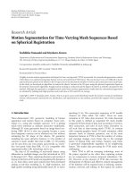
5.4.1. Frequency Response of an Exemplary Noise Reduction
System. We measured the frequency response of the noise
reduction system under test while high attenuation was
required in one subbband and no attenuation was required
in the other ones. In order to trigger this noise reduction
behavior on the one hand and to allow a measurement
over the whole bandwidth of the system on the other hand,
we used signal θ
b
according to (5) as a stimulus, where
parameter α in the synthesis of signal
s
b
via (4) was set to
zero.
Te s t
stimulus
D/A
L
1
M
2
L

2
M
1
A/D
Hearing
instrument
Noise reduction
system
Hard
disk
Figure 2: Measurement setup.
−8
−6
−4
−2
0
2
Gain (dB)
10
2
10
3
Frequency (Hz)
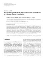
Frequency response
Figure 3: Measured frequency response of a noise reduction system
that is stimulated for attenuating one subband.
For each measurement, the test stimulus was presented
during 15 seconds in order to allow the system under test to
reach steady state. Bin-by-bin division of FFT absolute values
from the second measurement by corresponding values of

the first measurement delivered the frequency response of the
noise reduction system. Five FFT windows were averaged for
spectral smoothing [21].Thesewindowsweretakenfromthe
last five seconds of the test run in order to observe the steady-
state condition.
The result of this measurement is shown in Figure 3: the
shown frequency response indicates that the noise reduction
system under test provides attenuation in a subband around
800 Hz while not attenuating any other subband.
5.4.2. Attenuation Function of an Exemplar y Noise Reduction
System. We measured the dependency of attenuation on
modulation depth, where we defined that attenuation is the
average over the transfer function samples at frequencies
in a band of 100 Hz around the center frequency of the
subband of interest. One can argue that the narrow-band
signal
s
i
from (4) is the suitable stimulus for this kind of
measurement. However in our case, we based our stimulus
on

θ
b
from (6) in order to have a broadband stimulus
EURASIP Journal on Advances in Signal Processing 7
0
5
10
Attenuation (dB)

0 5 10 15 20
20 log
10
(1/[1 −α])
Attenuation versus modulation depth
Figure 4: Measured dependency of noise reduction attenuation on
modulation depth parameter 20
·log
10
([1 − α]
−1
).
with constant signal properties in most of the subbands.
This is an advantage when testing hearing instruments with
environment-dependent automatics, because the constant
subband signals we have in

θ
b
represent a defined environ-
ment, whereas
s
i
does not impose a defined environment on
any subband but the one of interest.
Measurements were performed with a modified version
of

θ
b

. The modification was to choose a sum index range of
(
{1, 2, , M}\{b −1, b, b +1}) instead of ({1,2, , M}\
{
b})from(6). This modification ensured that the nominal
frequency range of the band of interest spanned more than
one subband of the noise reduction system under test, thus
making the procedure invariant to clock differences between
the device under test and test equipment and to nonideal
subband split.
For the same reason, the band-stop filtering that is part
of (6) was made with a band-stop filter whose band limits
were set far enough outside the subbband of interest to reach
further than the filter slopes of the corresponding subband
split filter. We had to find a compromise between setting the
band limits of the band-stop filtering far outside the subband
of interest to make the measurement procedure robust and
setting them as close as possible to these band limits in order
to keep signal changes by the filtering as little as possible.
One reason to be careful with the choice of the stop-band
filter design is that the filtering can change the peak factor of
the synthesized stimuli (see also Section 3.4). As a result, we
chose band-stop corner frequencies that were half a subband
width away from the band limits of the subband of interest.
We u sed d ifferent test stimuli that resulted from varying
modulation parameter α according to (4). Since parameter
α is in the amplitude domain, whereas usual hearing
instrument specifications use decibels as unit, we used
20
· log

10
([1 − α]
−1
) rather than α as the modulation depth
parameter.
We var ied 20
·log
10
([1−α]
−1
) in steps of 2 and measured
the noise reduction attenuation as a function of this varied
parameter. The measured frequency response that was used
as a basis for computations was smoothed by averaging over
five FFT windows [21].
To obtain one single attenuation value from the fre-
quency response of interest, the proposed procedure from
Section 4 was used; this means that the frequency response
was searched for gain values corresponding to frequencies in
a
±50 Hz range around the center frequency of the subband
of interest, and the corresponding gain values were then
sorted and finally averaged after eliminating the first and last
quarter of the sorted list.
The obtained result is shown in Figure 4. We see that
the system under test behaves as one would expect of
a modulation-based noise reduction system (e.g., [8]):
Unmodulated signals are attenuated strongly, whereas mod-
ulated signals are not attenuated or attenuated less strongly.
6. Conclusion

Synthetic test signals have been proposed for verification
in the domain of digital hearing instruments. Discrete-
interval binary sequences have been used to synthesize
stimuli targeted at systematic verification of a modulation-
based noise reduction system.
Measurements with an exemplary hearing instrument
showed that the synthetic signals succeeded in both stim-
ulating the noise reduction in the subband of interest and
measuring the system’s frequency response and attenuation
function. With the given stimuli, it is possible to test against
specifications that require noise reduction attenuation as a
function of frequency and modulation.
References
[1] A. Schaub, Digital Hearing Aids, Thieme Medical, New York,
NY, USA, 2008.
[2] V. Harnacher, J. Chalupper, J. Eggers, et al., “Signal processing
in high-end hearing aids: state of the art, challenges, and future
trends,” EURASIP Journal on Applied Signal Processing, vol.
2005, no. 18, pp. 2915–2929, 2005.
[3] I. Holube, V. Hamacher, and M. Wesselkamp, “Hearing
instruments—noise reduction strategies,” in Proceedings of
the 18th Danavox Symposium on Auditory Models and Non-
linear Hearing Instruments, pp. 359–377, Kolding, Denmark,
September 1999.
[4] A. Kossiakoff and W. N. Sweet, Systems Engineer ing Principles
and Practice, John Wiley & Sons, Hoboken, NJ, USA, 2003.
[5] M. Marzinzik and B. Kollmeier, “Predicting the subjective
quality of noise reduction algorithms for hearing aids,” Acta
Acustica united with Acustica, vol. 89, no. 3, pp. 521–529, 2003.
[6] I. Holube, “Development and analysis of an international

speech test signal (ISTS),” in International Hearing Aid
Research Conference (IHCON ’08), Lake Tahoe, CA, USA,
August 2008.
[7] I. Holube and EHIMA-ISMADHA Working Group, “Short
description of the international speech test signal (ISTS),”
EHIMA—European Hearing Instrument Manufacturers
Association, (document contained in a download
package with the ISTS signal, April 2008), June 2007,
.
8 EURASIP Journal on Advances in Signal Processing
[8] R. Bentler and L K. Chiou, “Digital noise reduction: an
overview,” Trends in Amplification, vol. 10, no. 2, pp. 67–82,
2006.
[9] J. G. Lamm, A. K. Berg, and C. G. Gl
¨
uck, “Synthetic signals
for verifying noise reduction systems in digital hearing instru-
ments,” in Proceedings of the 16th European Signal Processing
Conference (EUSIPCO ’08), Lausanne, Switzerland, August
2008.
[10] P. E. Wellstead, “Pseudonoise test signals and the fast fourier
transform,” Electronic s Letters, vol. 11, no. 10, pp. 202–203,
1975.
[11] H. A. Barker and R. W. Davy, “System identification using
pseudorandom signals and the discrete fourier transform,”
Proceedings of the IEE, vol. 122, no. 3, pp. 305–311, 1975.
[12] H. W. Gierlich, “New measurement methods for determining
the transfer characteristics of telephone terminal equipment,”
in Proceedings of the IEEE International Symposium on Circuits
and Systems (ISCAS ’92), pp. 2069–2072, San Diego, CA, USA,

May 1992.
[13] M. R. Schroeder, “Synthesis of low-peak-factor signals and
binary sequences with low autocorrelation,” IEEE Transactions
on Information Theory, vol. 16, no. 1, pp. 85–89, 1970.
[14] R. Pintelon and J. Schoukens, System Identification: A Fre-
quency Domain Approach, IEEE Press, New York, NY, USA,
2001.
[15] E. Van der Ouderaa, J. Schoukens, and J. Renneboog, “Peak
factor minimization using a time-frequency domain swapping
algorithm,” IEEE Transactions on Instrumentation and Mea-
surement, vol. 37, no. 1, pp. 145–147, 1988.
[16] K. R. Godfrey, A. H. Tan, H. A. Barker, and B. Chong, “A
survey of readily accessible perturbation signals for system
identification in the frequency domain,” Control Engineering
Practice, vol. 13, no. 11, pp. 1391–1402, 2005.
[17] A. van den Bos and R. G. Krol, “Synthesis of discrete-interval
binary signals with specified fourier amplitude spectra,”
International Journal of Control, vol. 30, no. 5, pp. 871–884,
1979.
[18] K D. Paehlike and H. Rake, “Binary mutifrequency signals—
synthesis and application,” in Proceedings of the 5th IFAC
Symposium on Identification and System Parameter Estimation,
vol. 1, pp. 589–596, Darmstadt, Germany, September 1979.
[19] I. Koll
´
ar, Frequency Domain System Identification Toolbox V3.3
for Matlab, Gamax Ltd, Budapest, Hungary, 2004.
[20] S. T. Nichols and L. P. Dennis, “Estimating frequency-response
function using periodic signals and the f.f.t,” Electronics
Letters, vol. 7, no. 22, pp. 662–663, 1971.

[21] J. S. Bendat and A. G. Piersol, Random Data: Analysis and
Measurement Procedures, John Wiley & Sons, New York, NY,
USA, 2000.