Báo cáo hóa học: " Research Article Locally Regularized Smoothing B-Snake ´ ˆ Jerome Velut, Hugues Benoit-Cattin, and Christophe Odet" pptx

Hindawi Publishing Corporation
EURASIP Journal on Advances in Signal Processing
Volume 2007, Article ID 76241, 12 pages
doi:10.1155/2007/76241
Research Article
Locally Regularized Smoothing B-Snake
J
´
er
ˆ
ome Velut, Hugues Benoit-Cattin, and Christophe Odet
CREATIS, CNRS UMR 5220, Inserm U 630, INSA, B
ˆ
atiment Blaise Pascal, 69621 Villeurbanne, France
Received 22 July 2005; Revised 25 July 2006; Accepted 17 December 2006
Recommended by Jiri Jan
We propose a locally regularized snake based on smoothing-spline filtering. The proposed algorithm associates a regularization
process with a force equilibrium scheme leading the snake’s deformation. In this algorithm, the regularization is implemented with
a smoothing of the deformation forces. The regularization level is controlled through a unique parameter t hat can vary along the
contour. It provides a locally regularized smoothing B-snake that offers a powerful framework to introduce prior knowledge. We
illustrate the snake behavior on synthetic and real images, with global and local regularization.
Copyright © 2007 J
´
er
ˆ
ome Velut et al. This is an open access article distributed under the Creative Commons Attribution License,
which permits unrestricted use, distribution, and reproduction in any medium, provided the original work is properly cited.
1. INTRODUCTION
Active contour models (or snakes) are well adapted for
edge detection and segmentation. Since snakes were intro-
duced by Kass et al. [1], they have been widely used in

many domains and improved using different contour rep-
resentations and deformation algorithms. Menet et al. [2]
proposed the B-snakes that take advantages of the B-
spline representation. A local control of the curve con-
tinuity and a limited number of processed points in-
crease the convergence speed and the segmentation relia-
bility. At the same time, L. Cohen and I. Cohen [3]fo-
cused on external forces that drive the snake toward the
features of interest in the image and proposed the bal-
loon force that increases considerably the attainability zone.
Then, Xu and Prince [4] defined another external force
called gradient vector flow (GVF) that brings a better
control on the deformation directions: they proposed to
diffuse the gradient over the image according to optical
flow theory. Beside these works, the multiresolution f rame-
works were integrated within the active contours. Wang et
al. [5] used a B-spline representation that allows a coarse-
to-fine evolution of the snake. Brigger et al. [6, 7]ex-
tended Wang’s technique with a multiscale approach in
both the image and the parametric contour domain. Pre-
cioso et al. [8] proposed a region-based active contour that
achieves real-time computation adapted to video segmen-
tation. They extended their model by applying a smooth-
ing B-spline filter [9, 10] on the contour. It increases con-
siderably the robustness to noise without additional compu-
tation. Recently, new energies have been proposed by Jacob
et al. [11] who unify the edge-based scheme with the region-
based one.
Existing snakes suffer from several limitations when a lo-
cal regularization is wanted. With the original snake [1], a

local regularization involves a matrix inversion step at each
iteration. Although B-snakes [6] avoid this inversion step
by implicitizing the internal energy, the proposed solutions
induce a varying sampling step when a local regulariza-
tion of the snake is needed. Consequently, prior knowledge
would be difficult to integrate in the varying sampling step.
The smoothing B-spline filtering method of [8]doesnot
deal with local regularization and has a strong initialization-
dependent minimization process linked to the regularization
algorithm proposed.
In this paper, we propose to regularize local ly a snake
while keeping a uniform sampling step. The presented ap-
proach is based on smoothing-spline filtering that is con-
trolled through a unique parameter λ. The next section
reminds the snake concepts and their interaction with B-
splines. Section 3 details the proposed algorithm named
LRSB-snake that stands for locally regularized smoothing B-
snake. Section 4 presents experimental results on real and
synthetic images.
2. SNAKES AND B-SPLINES
First, we remind the original active contour of Kass et
al. [1] and its minimization procedure. Then, we present
the B-spline snake method and its evolutions. Afterward, we
2 EURASIP Journal on Advances in Signal Processing
describe the smoothing B-spline filtering strategy. Finally, we
analyze its usage within the smoothing-spline snake-based
algorithm of Precioso et al. [8].
2.1. Snakes: active contour model
Basically, a snake is a parametric curve g(s)
= (x(s), y(s))

placed on an image [1]. The final snake, that represents the
segmentation result, will be the curve that minimizes the en-
ergy E
snake
given by
E
snake
=

s
E
int

g(s)

+ E
ext

g(s)

ds,(1)
where
E
int
=
1
2

α(s) ·





dg(s)
ds




2
+ β(s) ·




d
2
g(s)
ds
2




2

,(2)
E
ext
=−



∇I(x, y)


2
. (3)
E
int
given by (2) is the internal energy that traduces shape
constraints on the curve. The α(s)andβ(s) functions tune
the regularization. The function β(s) gives more or less im-
portance to the curvature by weighting the second derivative
of the curve. In the same way, the function α(s) weights the
elasticity through a tuning of the first derivative. In order to
attract the snake to the contours of an image I, the external
energy E
ext
is defined in (3). Such energy is the most current
one. One can use any external energy expressions coherent
with the image features to detect.
In [1], the authors complete the minimization of the
E
snake
energy using the discretized version of (1):
E
snake
=

k

E
int

g(k)

+ E
ext

g(k)

,(4)
where k is the discretized version of the parameter s. This
leads to a force balance
A
· x + f
x
= 0, A · y + f
y
= 0, (5)
where A is a pentadiagonal banded matrix built from α(k)
and β(k) function v alues, where vectors x and y contain the
point coordinates of the discrete version g(k) of the curve
g(s), and where vectors f
x
and f
y
constitute the external forces
computed at the kth point of the snake as follows:
f (k)
=


f
x
(k), f
y
(k)

=

∂E
ext
(k)
∂x
,
∂E
ext
(k)
∂y

,(6)
where (x(k), y(k))
= g(k).
The equilibr ium state is reached using the gradient de-
scent method that ensures the convergence toward a local
minimum of energy:
A
· x
i
+ f
x,i−1

=−γ

x
i
− x
i−1

,
A
· y
i
+ f
y,i−1
=−γ

y
i
− y
i−1

,
(7)
where γ is a step-size parameter and i is the iteration index of
the gradient descent evolution.
c(k)
g(k)
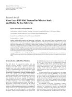
Figure 1: B-spline interpolation. c(k)arethecoefficients, g(k)are
the B-spline points, and g(s) is the curve that interpolates g(k).
We can then solve for x
i

and y
i
with x
i−1
and y
i−1
:
x
i
=

A + γI

−1

γ · x
i−1
− f
x,i−1

,
y
i
=

A + γI

−1

γ · y

i−1
− f
y,i−1

.
(8)
Solving this system iteratively leads to an equilibrium
state that is the minimum of the snake energy. Local min-
ima tra ps may be avoided with sufficient regularization, but
the need to initialize the snake close to the solution remains.
2.2. B-splines for B-snakes
The B-splines are continuous functions used to build para-
metric curves. The continuity is dependent on the degree of
the B-spline. Cubic B-splines are often used, because this is a
C
2
continuous function that provides an implicit smooth-
ness to adjacent points of the corresponding parametric
curve. A cubic uniform B-spline curve g(s)
= (x(s), y(s))
(Figure 1)isbuiltfromafinitesetofcoefficients c(k)with
x( s)
=
n−1

k=0
c
x
(k)B
k

(s), y(s) =
n−1

k=0
c
y
(k)B
k
(s), (9)
where n is the number of coefficients, B
k
(s) is the basis func-
tion centered on the kth coefficient.
The coefficients are represented through their plane co-
ordinates c(k)
= (c
x
(k), c
y
(k)).
Menetetal.[2] showed that (1) can be minimized
through an iterative process that is equivalent to (8)except
that the matrix A becomes A
b
and external forces f become
f
b
.ThematrixA
b
integrates the α and β coefficients of matrix

A and the first and second derivatives of the B-spline func-
tion. The new external forces f
b
(k) are derived from the ex-
ternal forces f (k) and the B-spline function B
k
.Thisiterative
J
´
er
ˆ
ome Velut et al. 3
g(k)
B
−1
(z)
c(k)
B(z)
g(k)
Figure 2: Block diagram of the direct and inverse B-spline filters.
g(k) are the curve points. B
−1
(z) is the direct B-spline filter that
computes the B-spline coefficients c(k)fromg(k). B(z) is the inverse
filter of B
−1
(z) and is called indirect B-spline filter.
process is given by
c
x,i

=

A
b
+ γI

−1

γ · c
x,i−1
− f
b
x,i
−1

c
y,i
=

A
b
+ γI

−1

γ · c
y,i−1
− f
b
y,i

−1

,
(10)
where c
x,i
and c
y,i
are vectors containing the coefficient val-
ues at iteration i. Such a snake is called B-snake in [2] and its
evolution is conducted using the coefficients values. More-
over, Flickner et al. [12] and Brigger et al. [6] use the built-in
smoothness property of the cubic B-splines to take the inter-
nal energy out of (1). The regularization is then controlled by
varying the distance between adjacent coefficients. The more
distant two coefficients are, the smoother the spline is. The
iterative system in (10) is then simplified by setting α and β
to0inA, and the iterative minimization process becomes
c
x,i
(k) = c
x,i−1
(k) −γ
−1
· f
b
x,i
−1
(k),
c

y,i
(k) = c
y,i−1
(k) −γ
−1
· f
b
y,i
−1
(k).
(11)
In [6], the authors prefer to interact with the snake via
real curve points instead of the coefficients. They implement
a digital filter B(z) described in [13] that links the B-spline
coefficients c(k) to the curve points g(k)by
g(k)
= b(k) ∗ c(k)
z
−→ G(z) = B(z) · C(z), (12)
where G(z), B(z), and C(z) are the Z-transforms of g(k),
b(k), and c(k)andwhere
B(z)
=
z +4+z
−1
6
. (13)
Using the inverse filter of B(z) allows one to obtain the B-
spline coefficients from the curve points (Figure 2). As coef-
ficients and curve points are linked together, there is no need

to work with B-spline coefficients in the deformation process
of the snake. Then (11) can be rewritten using the snake’s
point g( k) = (x(k), y(k)):
x
i
(k) = x
i−1
(k) −γ
−1
· f
x,i−1
(k),
y
i
(k) = y
i−1
(k) −γ
−1
· f
y,i−1
(k),
(14)
where x
i
(k)andy
i
(k) are the coordinates of the kth curve
point at iteration i.
2.3. Smoothing B-splines
B-splines interpolation is a mean of building continuous

curves from a finite set of coefficients. A B-spline interpolates
exactly a set of points g(k). However, an exact interpolation
is often not a reliable method of reconstruction. Reinsch [9]
illustrates this issue with a 1D signal taken from an imperfect
measuring tool. He proposed to approximate the set of mea-
sured points by spline functions. Given a set of points g( k),
the smoothing spline is the one that minimizes
ε
2
s
=
+∞

k=−∞

g(k) − g(k)

2
+ λ

+∞
−∞

∂
2
g(s)
∂
2
s


2
ds, (15)
where g(k) is the point set,
g(k) is the approximating point
set of g(k), and
g(s) is the continuous function that interpo-
lates
g(k).
The first term of (15) represents the error between the
original data set g(k) and the approximating one
g(k). The
second term, weighted by λ, represents the global curvature
of the curve. A large λ gives more impor tance to the smooth-
ing aspect of
g(k)whereasasmallλ imposes g(k) to be closer
to g(k). It is proven [9, 10] that a cubic B-spline is the solu-
tion of (15).
In [10], Unser et al. apply the B-spline filtering approach
to the smoothing spline formulation. They show that the co-
efficients of the approximating B-spline could be computed
through an IIR filter S
λ
. Consequently, from these approxi-
mating coefficients
c(k), one can find the approximating B-
spline points
g(k) through a B-spline filter B (Figures 3 and
4).
The smoothing B-spline filter transfer function is given
by

SB
λ
(z) = S
λ
(z) · B(z) =
z +4+z
−1
a + b ·

z + z
−1

+ c ·

z
2
+ z
−2

,
(16)
where
S
λ
(z) =
6
z +4+z
−1
+6· λ


z
2
− 4z +6− 4z
−1
+ z
−2

,
(17)
B(z)isgivenin(13), and a
= 4+36λ, b = 1−24λ,andc = 6λ.
SB
λ
(z) represents a fourth order symmetric filter with co-
efficients depending on λ. It is a low-pass filter with a cut-off
frequency controlled by λ (Figure 5). The link between λ and
the cut-off frequency f
c
with an attenuation of −3dBisgiven
by
λ

f
c

=
−
cos

2πf

c

+cos

2πf
c

√
2 − 2+2
√
2
12

cos

2πf
c

2
− 2cos

2πf
c

+1

,
f
c
(λ)

=
arccos

−
1+
√
2+24 ·λ+

3−2
√
2−144·λ+144
√
2·λ

/24·λ

2π
.
(18)
When λ equals 0, (34) shows that SB
λ
(z)equals1.It
means that
g(k) = g(k), that is, there is no approximation
(Figure 3).
In the time domain, the filtering is represented by a con-
volution equation involving the input signal g(k) and the
4 EURASIP Journal on Advances in Signal Processing
g(k)
g(s)

c(k)
(a)
g(k)
g(s)
c(k)
(b)
Figure 3: A smoothing B-spline curve. The points to approximate are the g(k) represented by the cross symbols. The c(k)arethecoefficients
of the smoothing B-spline and are represented by the dot symbols. The curve
g(s) is the approximating curve according to λ. (a) Approxi-
mation of a point set g(k) with λ
= 0. Note that in this case, we obtain a B-spline interpolation. (b) Approximation of the same point set
with λ
= 0.1.
g(k) S
λ
(z)
c(k)
B(z)
g(k)
SB
λ
(z)
λ
Figure 4: Block diagram of the smoothing B-spline filter SB
λ
. g(k)
are the curve points. S
λ
(z) is a filter that computes the smoothing
B-spline coefficients

c(k). B(z) is a filter that computes the B-spline
curve points from a set of coefficients.
g(k) are the approximating
points of g(k).
smoothed output g(k):
g(k) = g(k) ∗b(k) ∗ s
λ
(k) = g(k) ∗ sb
λ
(k), (19)
where sb
λ
(k) is the impulse response of the approximation
filter SB
λ
.
The implementation of the smoothing B-spline filter is
not straightforward. An efficient implementation was pro-
posed by Unser et al. [13]. It implements a causal/anticausal
filtering technique (see the appendix), resulting in O(n)com-
plexity of the filtering process, n being the number of points
of the input signal.
2.4. Smoothing B-splines and snakes
The smoothing-spline snake-based algorithm proposed by
Precioso et al. [8] takes advantage of the smoothness con-
trol allowed by a smoothing B-spline filter in the regulariza-
0
0.2
0.4
0.6

0.8
1
1.2
|SB
λ
|
00.10.20.30.4
Normalized frequency
λ
= 0
λ
= 0.1
λ
= 1
λ
= 10
λ
= 100
Figure 5: Frequency response of the smoothing-spline filter SB
λ
for
different values of λ.
tion of an active contour. The segmentation results obtained
with this algorithm show a good robustness to noise for λ
varying in the range [0.1, 1]. The authors underlined that
the computational cost of the contour smoothing is negli-
gible compared to the statistical evaluation involved in the
region-based active contour. This algorithm contains an ini-
tialization step, an evolution step, and a convergence test. Let
i be the iteration index, g(k) the sampling points,

c(k) the
smoothing spline coefficients.
At initialization step, we get g
i=0
(k) from an interface.
The smoothing spline coefficients are
c
i,0
(k) = s
λ
(k) ∗g
i,0
(k), (20)
where s
λ
(k) is the impulse response of S
λ
(z).
J
´
er
ˆ
ome Velut et al. 5
The snake evolution is conducted through the following
steps.
(a) Computation of the smoothing spline points:
g
i
(k) = b(k) ∗ c
i

(k). (21)
(b) Computation of evolution forces (d
i
(k)) according to
a region-based scheme detailed in [8]:
d
i
(k) = ν · N(k), (22)
where ν is defined as the velocity of the contour, N is
the normal vector to the contour.
(c) Displacement of
g
i
(k)byd
i
(k) to get the next points
g
i+1
(k):
g
i+1
(k) = g
i
(k)+d
i
(k). (23)
(d) Computation of smoothing spline coefficients:
c
i+1
(k) = s

λ
(k) ∗g
i+1
(k). (24)
(e) Return to step (a) until convergence.
The convergence test is based on some variation mea-
sures of the contour characteristics [8]. If an equilibrium cri-
terion is reached, the snake stops. We note that each iteration
involves a smoothing part represented by the convolution
equations (21)and(24), where b(k) is the impulse response
of the filter B(z), respectively. Introducing the iteration index
i and the deformation process through the evolution forces
(ν
· N
i
(k)) with respect to the algorithm, we obtain, from
(21)and(23),
g
i+1
(k) = g
i
(k)+d
i
(k) = c
i
(k) ∗b(k)+d
i
(k). (25)
From (25), we find
c

i+1
(k) = c
i
(k) ∗sb
λ
(k)+d
i
(k) ∗s
λ
(k), (26)
where d
i
(k) = ν · N
i
(k).
Finally, from (26) and using the Z transform, we obtain:

C
i+1
(z) =

C
0
(z) ·
i+1

SB
λ
(z)+
i


j=0

D
j
(z) ·S
λ
(z)
i−j

SB
λ
(z)

.
(27)
Equation (27) presents one term linked to the initial
smoothing-spline coefficients

C
0
(z) which is multiplied by
a product of the SB
λ
(z) approximation filter. As this filter is a
low-pass filter, the initial position of the snake tends to have
less importance when the number of iterations increases. A
similar behavior is observed within the second term of (26)
where the oldest deformation forces tend to be canceled. The
product terms involving the SB

λ
(z) approximation filter in
(27) explains the restricted range [0.1, 1] of the λ parame-
tervalues.Foragivennumberofiterations,greatervalues
of λ make the snake to shrink. The reproducibility of the re-
sults is hard to obtain because the SB
λ
regularization effect is
strongly linked to the number of iterations that is itself linked
to the initial position of the snake.
In this paper, we propose another approach that uses the
smoothing-spline filter in an active contour scheme where
λ values are not limited and where the regularization is not
iteration-dependent and can be locally defined.
InitializationDeformation
Convergence
Initial sampling points
g
0
(k)
Deformation forces computation
d
i
(k)
Deformation forces smoothing

d
i
(k) = sb
λ

∗ d
i
(k)
Moving sampling points
g
i+1
(k) =

g
i
+ μ ·

d
i
(k)
Resampling
No
i
= i +1
Convergence test
Yes
Segmentation ends
Figure 6: Flow-chart of the locally regularized smoothing B-snake
algorithm.
3. LOCALLY REGULARIZED SMOOTHING B-SNAKE
An overview of the proposed locally regularized Smoothing
B-Snake (LRSB-snake) is given in Figure 6. From an initial
contour
g
0

(k) and the image to segment, we compute the de-
formation forces (see Section 3.1). The regularization is done
by smoothing the defor mation forces. We can apply a global
regularization (Section 3.2) or a local one (Section 3.3). The
contour is then moved by applying the regularized deforma-
tion forces. To enforce a similar behavior of the smoothing
process at each iteration, the contour is resampled as dis-
cussed in Section 3.4. If the contour is stabilized, the iterative
processisstopped.
3.1. Deformation forces computation
The deformation of parametric models is performed by an
energy minimization [1]. The variational method used to
complete the minimization leads to the force balance given
by (5). This equation involves internal and external forces.
Internal forces that have a regularization role will be dis-
cussed in Section 3.2. This section focuses on external forces
and their usage as deformation vectors. The external forces
are directly derived from the image to segment. They guide
the snake to the desired features. Within the LRSB-snake al-
gorithm any type of external forces may be used. Basically, a
6 EURASIP Journal on Advances in Signal Processing
Laplacian vector field (6) computed from a Gaussian-blurred
version of the image gives suitable deformation forces [1]. Xu
and Prince proposed the gradient vector flow (GVF) [4]to
diffuse the gradient over the image in order to give a greater
range to the attraction forces. The balloon force [3]isan-
other external force. It is a vector directed along the normal
of the contour. It creates a pressure force at each point of the
snake that makes it swelling.
The sum of every considered forces gives the deformation

vector d
i
(k)ateachpointk andateachiterationi. As the
basic idea of a deformation process is to move every point
according to a deformation vector, we define the following
deformation equation:
g
i+1
(k) = g
i
(k)+μ ·d
i
(k), (28)
where i is the iteration index, g(k) are the snake points, d
i
(k)
are the deformation vectors, that is, the external forces, and μ
is a step-size parameter involved in the speed of convergence.
Equation (10) corresponds to (28)ifwesetμ
=−γ
−1
and
d(k)
= f (k). Note that (28) does not imply any regulariza-
tion process.
3.2. Global regularization process through
deformation forces smoothing
Regularization of the deformable model is essential to ensure
a good robustness to noise of such segmentation approach.
Usually, the regularization is assumed through an internal

energy term in the snake energy formulation [1] or implicitly
through a variation of the contour sampling [6]. Such regu-
larization prevents incoherent deformation of the contour by
introducing a curvature-based penalty. We choose to control
the curvature of the contour with a smoothing B-spline fil-
ter that minimizes the curvature optimally [9] according to a
single parameter λ.
Equation (29) gives the snake regularized by the SB
λ
ap-
proximation filter at iteration i,
g
i
(k) = sb
λ
(k) ∗g
i
(k). (29)
From (28)and(29), we obtain (30) that yields the defor-
mation and the motion steps of the algorithm (Figure 6),
g
i+1
(k) = g
i
(k)+

μ · d
i
(k)


∗
sb
λ
(k). (30)
Finally, from (30) and using the Z-transform, we obtain

G
i+1
(k) =

G
0
(k)+μ ·
i

j=0
D
j
(z) ·SB
λ
(z). (31)
It is clear in (30) that we bring into effect the snake regu-
larization by a smoothing filtering of the deformation forces
(Figure 6). Consequently (31), an infinite iterative process
does not lead to an infinite successive convolution of d
i
.
Compared to [8], the regularization does not depend on the
number of iterations. It allows λ to control the cut-off fre-
quency of the SB

λ
approximation filter and thus the regular-
ization level by taking any real positive values. As the regu-
larization is done by a digital recursive filter, it preserves the
processing speed mentioned in [8].
In practice, the 1D smoothing B-spline filter is used to
filter a parametric curve in the plane. It is applied on each
parametr ic component of the curve as in (32). Figure 7 illus-
trates the filtering of such a parametric curve,
g(k) = sb
λ
(k) ∗g(k) =⇒


g
x
(k)
g
y
(k)

=

sb
λ
(k) ∗g
x
(k)
sb
λ

(k) ∗g
y
(k)

.
(32)
Note that a 1-D filter is usually applied on a uniformly
sampled signal. As we want to keep the same filter frequency
response which is λ-dependent, we enforce a uniform sam-
pling of the contour in our algor ithm (see Section 3.4).
3.3. Local regularization process
From the regularization term of (30), one can write the fol-
lowing equation:

D
i
(z) = SB
λ
(z) ·D
i
(z), (33)
where
SB
λ
(z) = S
λ
(z) · B(z) =
z +4+z
−1
a + b ·


z + z
−1

+ c ·

z
2
+ z
−2

(34)
with a
= 4+36λ, b = 1 − 24λ,andc = 6λ.
In (Appendix A.2), we show that (33)conductstotwo
recurrence equations (A.10)and(A.11) where the filters co-
efficients a, b,andc appears. We propose to make those two
equations space-varying by making λ dependent of the kth
contour point. Thus, a, b,andc become
a
k
= 4+36·λ
k
, b
k
= 1 − 24 · λ
k
, c
k
= 6 · λ

k
(35)
and the space-varying recurrence equations are

d
1
(k) = c
k
· d(k)+a
k
·

d
1
(k − 1) − b
k
·

d
1
(k − 2),

d
2
(k) = c
k
·

d
1

(k)+a
k
·

d
2
(k +1)− b
k
·

d
2
(k +2).
(36)
Consequently, each point of the snake has its own regu-
larization rate. We are able to affect different values of λ along
the contour (Figure 8) according to several strategies like lo-
cal image information (to adapt λ to noise level or to perti-
nent image features under the contour), or prior knowledge
introduced in the initial model (to keep the contour in a con-
trolled deformation range). These strategies may have differ-
ent impacts on snake evolution that are beyond the scope of
this paper.
3.4. Resampling
For a given λ the contour sampling rate has to be constant to
keep the same cut-off frequency of the smoothing filter (see
Section 2.3) and consequently the same regular ization effect.
Our algorithm implements a resampling step at each itera-
tion (Figure 6) to get a constant distance between the con-
tour points. We do not implement a subdivision scheme, but

J
´
er
ˆ
ome Velut et al. 7
(a) (b)
(c) (d)
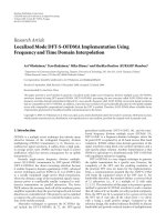
Figure 7: Smoothing B-spline filtering of a parametric circle with parameter s. Noisy circle in (b) is described by x(s)andy(s)(a).Thecircle
in (b) has a constant radius disturbed by a uniformly distributed additive noise. x(s)andy(s) are smoothed separately by the smoothing
B-spline filter (c). (d) shows the smoothed parametric circle.
λ = 50
λ
= 1
λ
= 50 000
Figure 8: Spatially variant smoothing-spline filtering. The input
signal is the noisy circle. This signal is filtered through a smoothing-
spline filter where the smoothing parameter λ varies along the con-
tour. The resulting signal is represented in bold.
a resampling one. Starting with one existing point, each next
point is set at a fixed distance from the previous one as de-
scribed in the following algorithm.
Let g(s) be the original contour, g

(i) the resampled con-
tour , i the new point index, s the continuous parameter, e
the wanted constant sampling distance, and N the number
of points of the original contour. N
− 1 represents also the
total curve length.

(1) Initialization: g

(0) = g(0), i = 0.
(2) Incrementation of i.
(3) Find s such that
g(s)g

(i − 1)=e, then set g

(i) =
g(s).
(4) Repeat steps (2) and (3) while s<N
− 1.
As g

(i) = (x

(i), y

(i)), we have g

(i)g

(i − 1)=

(x

(i) − x

(i − 1))

2
+(y

(i) − y

(i − 1))
2
.
The resampling impact is illustrated in Figure 9 where
acurvewithdifferent sampling rates is smoothed via a
smoothing B-spline filter with the same λ. It appears that
the greatest interpoint distance (Figure 9(d)) leads to the
smoothest curve.
When λ is locally variant, the λ-values under the new
points are obtained by linear interpolation between the λ-
values of the previous and the next old points.
3.5. Open and closed contours
The smoothing-spline filter has an infinite impulse response.
To implement the corresponding difference equation (33),
Unser et al. [13] proposed to initialize the filtering process
with an approximation of the impulse response. Boundary
conditions have to be clearly defined in order to choose a cor-
rect extrapolation of the signal.
If we consider a closed contour, the signal g(k)ismade
periodic. Thus the extrapolation may be seen as a mod-
ulo function that is well adapted to closed contour. The
smoothed circle in Figure 9 is obtained in such a way.
8 EURASIP Journal on Advances in Signal Processing
(a)Standard curve to be smoothed. (b)10 000-point smoothed curve.
(c)1000-point smoothed curve. (d)100-point smoothed curve.

Figure 9: Illustration of the influence of sampling over the λ value. Each curve is smoothed by the same smoothing B-spline filter with
λ
= 1000.
Figure 10: Illustration of an opened contour smoothing using an
antimirror with pivot point extension. A hand-drawn line and its
smoothed version are given.
The open contour case is different because we need to ex-
trapolate the parametric signal while keeping a suitable con-
tinuity at endpoints. Several extrapolation techniques have
been proposed leading to different behaviors [6, 14]. We
choose to implement an antisymmetric mirror with pivot
point extension [6] in order to conserve the continuity at ex-
treme points. A smoothed open contour including such an
extension is illustrated in Figure 10.
4. RESULTS
This section gives results obtained with the proposed LRSB-
snake algorithm. First, the global regularization mode is il-
lustrated using real MRI images with opened and closed con-
tours. Then, the LRSB-snake is applied on synthetic image
and real MRI image to illustrate the advantage of such a local
regularization. All these results have been obtained with the
following external forces: Laplacian vectors of a Gaussian-
blurred version of the image combined with a balloon force
to increase the convergence speed.
4.1. Global regularization
Figure 11(a) shows an MR image of a guinea-pig knee and
an initial opened smoothing B-snake. The feature to detect is
the femoral border. With a too low λ value (λ
= 71), the final
result obtained after 1280 iterations is corrupted by a local

minimum (Figure 11(c)). We set a larger λ value (λ
= 1000)
to avoid this ar tifact (Figure 11(c)). The final result obtained
after 630 iterations is close to the wanted femora l border.
Figure 12 shows an anatomic struc ture in an MRI an-
giography. This structure presents an upper-right protuber-
ance and a lack of gray-level gradient in the bottom right
place. Figure 12 illustrates the algorithm behavior with a
global regularization and a closed contour. With λ
= 200
(Figure 12(c)), the right upper part of the anatomic structure
is missing and the final position is not correct at the bottom
right, after 550 iterations. A correct segmentation is obtained
J
´
er
ˆ
ome Velut et al. 9
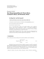
(a) Initial snake. (b) λ = 1000, 630 iterations. (c) λ = 71, 1280 iterations.
Figure 11: MRI image of a guinea-pig knee and an initial 67 points snake.
(a) Initial snake. (b) λ = 12, 550 iterations. (c) λ = 220, 480 iterations.
Figure 12: Segmentation of an MRI image through a close snake. Final snakes are 150 points long.
(Figure 12(b))withalowervalueofλ (λ = 12) and 480 iter-
ations.
4.2. Local regularization
To illustrate the limitation of the global regularization, we
use a synthetic image obtained from a circle (Figure 13(a)).
The circle contour is modulated to introduce as many ranges
of curvature variation as there are different modulation fre-
quencies. A Gaussian noise is then added to the image. Global

regularization demonstrates its limits on Figures 13(b) and
13(c). A low global λ value leads to an evolution of the con-
tour very sensitive to noise. The snake may be stuck in local
minima as in Figure 13(b). A large global λ value induces too
much constraint on the snake curvature. The final contour
could only outline a mean circle (Figure 13(c)).
On Figure 13(d), we use the locally regularized scheme
where λ was made spatially variant. The highest frequency
part (I) was attached to a low λ (λ
= 1). We then increase λ
to 10 in order to outline successfully the second part (II) of
the disk. Last part (III) being perfectly circular, λ was set to
100.
We note with these tests that the LRSB-snake provides
a segmentation result (Figure 13(d)) closest to the object to
outline (white contour in Figure 13(a)).
Figure 14 illustrates the same behavior on a real MRI im-
age that presents interesting features: an unsharp gradient
area (“ghost gradient”) at the top of the shape that is not an
edge to outline and a lack of gradient at middle right. On
Figure 14(b), balloon forces induce a leak of the snake which
is not sufficiently regularized. The ghost gradient corrupts
the final result also by introducing a curve that does not ex-
ist. A larger λ value (Figure 14(c)) prevents the leak but gives
too much importance to the unsharp gradient area.
The LRSB-snake is then applied on this image
(Figure 14(d)). A λ map gives the λ values at each im-
age position. In this example, the λ map is manually defined,
with values empirically determined as follows. Positions
where the contour is well visible take a small λ value (λ

= 1),
and positions where the contour tends to disappear take a
high λ value (λ
= 300). One can observe on Figure 14(d)
that such a local regularization prevents the leak, manages
correctly the ghost gradient, and stops the swell at the top.
A strategy to automatically define λ variations is beyond the
scope of this paper.
5. CONCLUSIONS
In this paper, we propose a locally regularized smoothing B-
snake algorithm. The regularization process uses an approx-
imating smoothing-spline filter applied directly on the snake
point displacement. This algorithm conser ves the advantages
of snake algorithms and offers a local control of the regular-
ization through the λ value defined at each snake points. As
the regularization is implemented through a recursive imple-
mentation of a digital filter, this algorithm is fast.
10 EURASIP Journal on Advances in Signal Processing
(a) (b)
(c)
I
II
III
(d)
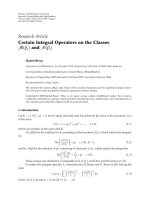
Figure 13: Constant and locally regularized 100-points s moothing B-snake on a synthesis image. (a) Noisy object with the reference contour
in white. (b) Final segmentation with global low λ (λ
= 1). (c) Final segmentation with global high λ (λ = 100). (d) Locally regularized
smoothing B-Snake. (I : λ
= 1, II : λ = 10, III : λ = 100).
(a) (b) (c) (d)

Figure 14: Constant and local regularization on an MRI image. (a) Initial snake and original MRI image. (b) Final segmentation after 310
iterations using λ
= 1. (c) Final segmentation after 250 iterations using λ = 300. (d) Final segmentation after 330 iterations using local λ
values (black for λ
= 300, white for λ = 1).
J
´
er
ˆ
ome Velut et al. 11
This algorithm associated to pertinent local λ definition
offers a powerful tool for introducing prior knowledge and
consequently makes the segmentation process more robust.
A. APPENDIX
This appendix details the smoothing B-spline filter imple-
mentation which is linked to the λ value that impacts the
filter pole values.
A.1. Smoothing B-spline filter pole analysis
We implement the smoothing spline-filter as discussed in
[13]. The filtering system is the one presented in Figure 4.
The B(z) filter is an FIR filter and is implemented through
the difference equation associated to its transfer function
(13). The S(z) filter implementation is not straightforward
because of its transfer function (17). The S(z)filterisequiv-
alent to a cascade of two symmetric second-order filters:
S
λ
(z) = S
+
λ

(z) · S
+
λ

z
−1

(A.1)
with
S
+
λ
(z) =
1 − 2ρ · cos(ω)+ρ
2
1 − 2ρ · cos(ω) ·z
−1
+ ρ
2
· z
−2
. (A.2)
In (A.2), ρ and ω are the magnitude and argument of the
two complex conjugate roots (p
1
= ρ exp
jω
, p
2
= ρ exp

−jω
)
of the S
+
λ
(z) denominator, and they are linked to the λ value
by
ρ
=
24λ − 1 −

ξ
24λ
·



48λ +24λ ·
√
3 + 144λ
ξ
,
tan (ω)
=

144λ − 1
ξ
,
(A.3)
ξ

= 1 − 96λ +24λ ·

3 + 144λ. (A.4)
Equations (A.3)arevalidforλ value greater than 1/24.
For other λ values several cases have to be considered.
(1) When λ
= 1/24, ρ and ω take the specific values given
by
ρ
=

11 −
√
120,
ω
=
π
2
.
(A.5)
(2) When λ value belongs to the interval ]1/144 : 1/24[,
(A.3) are still valid but ρ value is greater than one, and
consequently the associated conjugate roots are the roots of
S
+
λ
(z
−1
) instead of being those of S
+

λ
(z).
(3) When λ value belongs to the interval ]0 : 1/144], the
roots of S
+
λ
(z)becomerealandaregivenby
p
1
=
2+x
1
+

4x
1
+ x
2
1
2
, p
2
=
2+x
2
+

4x
2
+ x

2
2
2
(A.6)
with x
1
= (−1+
√
1 − 144λ)/12λ and x
2
= (−1−
√
1 − 144λ)/
12λ.
Then, we can write S
+
λ
(z) as follows:
S
+
λ(z) =

p
1
p
2
λ
1
1 −


p
1
p
2

z
−1
+ p
1
p
2
z
−2
. (A.7)
(4) When λ value equals 0, we have
λ
= 0 ⇐⇒ S
λ
(z) = B
−1
(z) ⇐⇒ SB
λ
(z) = 1. (A.8)
It means that the smoothing B-spline filter has no effect:
input and output signals are equal.
A.2. Smoothing B-spline filter implementation
The filter SB(z) is implemented as a cascade of two
causal/anticausal filters (A.1) followed by the filter B(z)(13),

D

1
(z) = D( z) · S
+
λ
(z),

D
2
(z) =

D
1
(z) · S
+
λ

z
−1

,
D(z)
=

D
2
(z) ·B(z).
(A.9)
The corresponding difference equations are given by

d

1
(k) = c · d(k)+a ·

d
1
(k − 1) − b ·

d
1
(k − 2), (A.10)

d
2
(k) = c ·

d
1
(k)+a ·

d
2
(k +1)− b ·

d
2
(k + 2), (A.11)

d(z) =
1
6



d
2
(k − 1) + 4 +

d
2
(k +1)

, (A.12)
where a, b,andc are computed from ρ and ω depending
on the λ value as detailed in the previous appendix section.
Equation (A.10) represents the causal filtering while (A.11)
represents the anticausal one. This is implemented by revers-
ing the signal

d
1
(k), filtering it with S
+
λ
and reversing the out-
put.
As the smoothing B-spline filter is an IIR filter, the com-
putation of the output at instant k requires the output knowl-
edge at instants k
− 1andk − 2((A.10)and(A.11)). Conse-
quently, the filtering process has to be initialized for the two
first points (in the causal recursion) and the two last ones (in

the anticausal recursion). For these initializations, we use an
approximation of the impulse response of S
+
λ(z):

d
1
(0) =
n

k=0
d(k)s
+
λ
(k),

d
1
(1) =
n

k=0
d(k)s
+
λ
(k − 1),
(A.13)
where n is the length of the approximation. Note that n
should be sufficiently high to correctly approximate the im-
pulse response. Consequently, n value will be increased w ith

the λ value. The anticausal filtering is initialized equivalently.
When λ>1/144, the impulse response is given by
s
+
λ
(k) =

1 − 2ρ · cos (ω)+ρ
2

ρ
|k|
sin

|
k|+1

ω

sin (ω)
.
(A.14)
12 EURASIP Journal on Advances in Signal Processing
When λ<1/144, the impulse response is given by
s
+
λ
(k) =

p

1
p
2
λ

1
1 − p
2
/p
1
p
|k|
1
+
1
1 − p
1
/p
2
p
|k|
2

.
(A.15)
When λ
= 1/144, the impulse response is given by
s
+
λ

(k) =

|
k|+1

·
p
|k|
1
. (A.16)
ACKNOWLEDGMENTS
This work is in the scope of the scientific topics of the PRC-
GdR ISIS Research Group of the French National Center for
Scientific Research CNRS. We would like to thank the review-
ers of this paper for their comments and suggestions.
REFERENCES
[1] M. Kass, A. Witkin, and D. Terzopoulos, “Snakes: active con-
tour models,” in Proceedings of the 1st International Conference
on Computer Vision, pp. 259–268, London, UK, June 1987.
[2] S. Menet, P. Saint-Marc, and G. Medioni, “B-snakes: imple-
mentation and application to stereo,” in Proceedings of Image
Understanding Workshop, pp. 720–726, Pittsburgh, Pa, USA,
September 1990.
[3] L. D. Cohen and I. Cohen, “Finite-element methods for ac-
tive contour models and balloons for 2-D and 3-D images,”
IEEE Transactions on Pattern Analysis and Machine Intelligence,
vol. 15, no. 11, pp. 1131–1147, 1993.
[4] C. Xu and J. L. Prince, “Snakes, shapes, and gradient vector
flow,” IEEE Transactions on Image Processing, vol. 7, no. 3, pp.
359–369, 1998.

[5] M. Wang, J. Evans, L. Hassebrook, and C. Knapp, “A multi-
stage, optimal active contour model,” IEEE Transactions on Im-
age Processing, vol. 5, no. 11, pp. 1586–1591, 1996.
[6] P. Brigger, J. Hoeg, and M. Unser, “B-spline snakes: a flexible
tool for parametric contour detection,” IEEE Transactions on
Image Processing, vol. 9, no. 9, pp. 1484–1496, 2000.
[7] P. Brigger and M. Unser, “Multi-scale B-spline snakes for gen-
eral contour detection,” in Wavelet Applications in Sig nal and
Image Processing VI, vol. 3458 of Proceedings of SPIE, pp. 92–
102, San Diego, Calif, USA, July 1998.
[8] F. Precioso, M. Barlaud, T. Blu, and M. Unser, “Robust real-
time segmentation of images and videos u sing a smooth-
spline snake-based algorithm,” IEEE Transactions on Image
Processing, vol. 14, no. 7, pp. 910–924, 2005.
[9] C. H. Reinsch, “Smoothing by spline functions,” Numerische
Mathematik, vol. 10, no. 3, pp. 177–183, 1967.
[10] M. Unser, A. Aldroubi, and M. Eden, “B-spline signal
processing—part I. Theory,” IEEE Transactions on Signal Pro-
cessing, vol. 41, no. 2, pp. 821–833, 1993.
[11] M. Jacob, T. Blu, and M. Unser, “Efficient energies and al-
gorithms for parametric snakes,” IEEE Transactions on Image
Processing, vol. 13, no. 9, pp. 1231–1244, 2004.
[12] M. Flickner, H. Sawhney, D. Pryor, and J. Lotspiech, “Intelli-
gent interactive image outlining using spline snakes,” in Pro-
ceedings of the 28th Asilomar Conference on Sig nals, Systems
and Computers, vol. 1, pp. 731–735, Pacific Grove, Calif, USA,
October-November 1994.
[13] M. Unser, A. Aldroubi, and M. Eden, “B-spline signal
processing—part II. Efficient design and applications,” IEEE
Transactions on Signal Processing, vol. 41, no. 2, pp. 834–848,

1993.
[14] L. Weruaga, R. Verd
´
u, and J. Morales, “Frequency domain
formulation of active parametric deformable models,” IEEE
Transactions on Pattern Analysis and Machine Intelligence,
vol. 26, no. 12, pp. 1568–1578, 2004.
J
´
er
ˆ
ome Velut graduated in 2003 as a Com-
puting Engineer from the Universit
´
ede
Provence (France). He then specialized in
image processing at the INSA, Lyon, and re-
ceived the Master degree in image and sys-
tem in 2004. Since this graduation, he is a
Ph.D. student at the Research and Applied
Image and Signal Processing Center (CRE-
ATIS) at the INSA, Lyon. His research inter-
ests include image processing, deformable
models, and 3D modeling.
Hugues Benoit-Cattin received in 1992
the Engineer degree (electrical engineering)
and in 1995 the Ph.D. degree (wavelet im-
age coding of medical images), both from
INSA, Lyon, France. He is Associated Pro-
fessor at INSA, Lyon, at the Telecommu-

nications Department. His teaching activi-
ties mainly concern information theory, sig-
nal and image processing. He worked since
1992 at CREATIS Laboratory (CNRS no.
5515 INSERM U630). For six years (1992–1998), he worked on
image coding including DCT, wavelet- and fractal-based coding
schemes applied to medical images and spatial images. Since 1998,
he is member of the Volumic Imaging Research Team of CREATIS.
His main research interests include image segmentation as well as
MRI image acquisition, correction, and simulation.
Christophe Odet received in 1979 the Engi-
neering degree (electrical engineering) and
in 1984 the Ph.D. degree (nondestructive
testing), both from the National Institute
for Applied Sciences of Lyon (France). He
worked since 1984 at CREATIS as Assistant
Professor. His primary research interests in-
cluded image segmentation and classifica-
tion based on texture analysis and signal
and image restoration. He has been involved
in the application of the previous methods to linear and 2D image
sensors for the control of high-speed moving products. He is n ow
Professor at CREATIS and is mainly involved in image processing
and segmentation for medical and biological applications such as
bone analysis or small animals imaging.