Báo cáo hóa học: " Research Article Towards Structural Analysis of Audio Recordings in the Presence of Musical Variations" docx

Hindawi Publishing Corporation
EURASIP Journal on Advances in Signal Processing
Volume 2007, Article ID 89686, 18 pages
doi:10.1155/2007/89686
Research Article
Towards Structural Analysis of Audio Recordings in
the Presence of Musical Variations
Meinard M
¨
uller and Frank Kurth
Department of Computer Science III, University of Bonn, R
¨
omerstraße 164, 53117 Bonn, Germany
Received 1 December 2005; Revised 24 July 2006; Accepted 13 August 2006
Recommended by Ichiro Fujinaga
One major goal of structural analysis of an audio recording is to automatically extract the repetitive structure or, more generally,
the musical form of the underlying piece of music. Recent approaches to this problem work well for music, where the repetitions
largely agree with respect to instrumentation and tempo, as is typically the case for popular music. For other classes of music such
as Western classical music, however, musically similar audio segments may exhibit significant variations in parameters such as
dynamics, timbre, execution of note groups, modulation, articulation, and tempo progression. In this paper, we propose a robust
and efficient algorithm for audio structure analysis, which allows to identify musically similar segments even in the presence
of large variations in these parameters. To account for such variations, our main idea is to incorporate invariance at vari ous
levels simultaneously: we design a new type of statistical features to absorb microvariations, introduce an enhanced local distance
measure to account for local variations, and describe a new strategy for structure extraction that can cope with the global variations.
Our experimental results with classical and popular music show that our algorithm performs successfully even in the presence of
significant musical variations.
Copyright © 2007 M. M
¨
uller and F. Kurth. This is an open access article distributed under the Creative Commons Attribution
License, which permits unrestricted use, distribution, and reproduction in any medium, provided the original work is properly
cited.

1. INTRODUCTION
Content-based document analysis and efficient audio brows-
ing in large music databases has become an important issue
in music information retrieval. Here, the automatic annota-
tion of audio data by descriptive high-level features as well
as the automatic generation of crosslinks between audio ex-
cerpts of similar musical content is of major concern. In this
context, the subproblem of audio structure analysis or, more
specifically, the automatic identification of musically relevant
repeating patterns in some audio recording has been of con-
siderable research interest; see, for example, [1–7]. Here, the
crucial point is the notion of similar ity used to compare dif-
ferent audio segments, because such segments may be re-
garded as musically similar in spite of considerable variations
in parameters such as dynamics, timbre, execution of note
groups (e.g., g race notes, trills, arpeggios), modulation, ar-
ticulation, or tempo progression. In this paper, we introduce
arobustandefficient algorithm for the structural analysis
of audio recordings, which can cope with sig nificant vari-
ations in the parameters mentioned above including local
tempo deformations. In particular, we introduce a new class
of robust audio features as wel l as a new class of similarity
measures that yield a high degree of invariance as needed to
compare musically similar segments. As opposed to previous
approaches, which mainly deal with popular music and as-
sume constant tempo throughout the piece, we have applied
our techniques to musically complex and versatile Western
classical music. Before giving a more detailed overview of our
contributions and the structure of this paper (Section 1.3),
we summarize a general strateg y for audio structure anal-

ysis and introduce some notation that is used throughout
this paper (Section 1.1). Related work will be discussed in
Section 1.2.
1.1. General strategy and notation
To extr act the repetitive structure from audio signals, most
of the existing approaches proceed in four steps. In the first
step, a suitable high-level representation of the audio signal is
computed. To this end, the audio signal is transformed into a
sequence

V :
= (

v
1
,

v
2
, ,

v
N
)offeaturevectors

v
n
∈ F ,
1
≤ n ≤ N.Here,F denotes a suitable feature space,

for example, a space of spectral, MFCC, or chroma vectors.
2 EURASIP Journal on Advances in Sig nal Processing
Based on a suitable similarity measure d : F × F → R
≥0
,
one then computes an N-square self-similarity
1
matrix S de-
fined by S(n, m):
= d(

v
n
,

v
m
), effectively comparing all fea-
ture vectors

v
n
and

v
m
for 1 ≤ n, m ≤ N in a pairwise fash-
ion. In the third step, the path structure is extracted from the
resulting self-similarity matrix. Here, the underlying princi-
ple is that similar segments in the audio signal are revealed

as paths along diagonals in the corresponding self-similarity
matrix, where each such path corresponds to a pair of simi-
lar segments. Finally, in the four th step, the g lobal repetitive
structure is derived from the information about pairs of sim-
ilar segments using suitable clustering techniques.
To illustrate this approach, we consider two examples,
which also serve as running examples throughout this pa-
per. The first example, for short referred to as Brahms ex-
ample, consists of an Ormandy interpretation of Brahms’
Hungarian Dance no. 5. This piece has the musical form
A
1
A
2
B
1
B
2
CA
3
B
3
B
4
D consisting of three repeating A-parts
A
1
, A
2
,andA

3
, four repeating B-parts B
1
, B
2
, B
3
,andB
4
,as
well as a C-andaD-part. Generally, we will denote musical
parts of a piece of music by capital letters such as X,where
all repetitions of X are enumerated a s X
1
, X
2
, and so on. In
the following, we will distinguish between a piece of music (in
an abstract sense) and a particular audio recording (a con-
crete interpretation) of the piece. Here, the term part will be
used in the context of the abstract music domain, whereas
the term segment will be used for the audio domain.
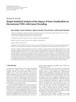
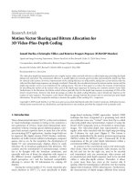
The self-similarity matrix of the Brahms recording (with
respect to suitable audio features and a particular similarity
measure) is shown in Figure 1. Here, the repetitions implied
by the musical form are reflected by the path structure of the
matrix. For example, the path starting at (1,22) and ending at
(22, 42) (measured in seconds) indicates that the audio seg-
ment represented by the time interval [1 : 22] is similar to
the segment [22 : 42]. Manual inspection reveals that the

segment [1 : 22] corresponds to part A
1
, whereas [22 : 42]
corresponds to A
2
. Furthermore, the curved path starting
at (42, 69) and ending at (69, 89) indicates that the segment
[42 : 69] (corresponding to B
1
) is similar to [69 : 89] (cor-
responding to B
2
). Note that in the Ormandy interpretation,
the B
2
-part is played much faster than the B
1
-part. This fact
is also revealed by the gradient of the path, which encodes the
relative tempo difference between the two segments.
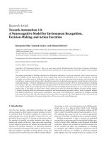
As a second example, for short referred to as Shostakovich
example, we consider Shostakovich’s Waltz 2 from his Jazz
Suite no. 2 in a Chailly interpretation. This piece has the
musical form A
1
A
2
BC
1
C

2
A
3
A
4
D, where the theme, repre-
sented by the A-part, appears four times. However, there are
significant variations in the four A-parts concerning instru-
mentation, articulation, as well as dynamics. For example,
in A
1
the theme is played by a clarinet, in A
2
by strings, in
A
3
by a trombone, and in A
4
by the full orchestra. As is il-
1
In this paper, d is a distance measure rather than a similarity measure as-
suming small values for similar and large values for dissimilar feature vec-
tors. Hence, the resulting matrix should strictly be called distance matrix.
Nevertheless, we use the term similarity matrix according to the standard
term used in previous work.
20
40
60
80
100

120
140
160
180
200
50 100 150 200
A
1
A
2
B
1
B
2
C
A
3
B
3
B
4
D
A
1
A
2
B
1
B
2

CA
3
B
3
B
4
D
Figure 1: Self-similarity matrix S[41, 10] of an Ormandy interpre-
tation of Brahms’ Hungarian Dance no. 5. Here, dark colors corre-
spond to low values (high similarity) and light colors correspond to
high values (low similarity). The musical form A
1
A
2
B
1
B
2
CA
3
B
3
B
4
D
is reflected by the path structure. For example, the curved path
marked by the hor izontal and vertical lines indicates the similarity
between the segments corresponding to B
1
and B

2
.
lustrated by Figure 2, these variations result in a fragmented
path structure of low quality, making it hard to identify the
musically similar segments [4 : 40], [43 : 78], [145 : 179],
and [182 : 217] corresponding to A
1
, A
2
, A
3
,andA
4
,respec-
tively.
1.2. Related work
Most of the recent approaches to structural audio analysis fo-
cus on the detection of repeating patterns in popular music
based on the strategy as described in Section 1.1. The concept
of similarity matrices has been introduced to the music con-
text by Foote in order to visualize the time structure of audio
and music [8]. Based on these mat rices, Foote and Cooper
[2] report on first experiments on automatic audio summa-
rization using mel frequency cepstral coefficients (MFCCs).
To allow for small variations in performance, orchestration,
and lyrics, Bartsch and Wakefield [1, 9] introduced chroma-
based audio features to structural audio analysis. Chroma
features, representing the spectral energy of each of the 12
traditional pitch classes of the equal-tempered scale, were
also used in subsequent works such as [3, 4]. Goto [4]de-

scribes a method that detects the chorus sections in audio
recordings of popular music. Important contributions of this
work are, among others, the automatic identification of both
ends of a chorus section (without prior knowledge of the
chorus length) and the introduction of some shifting tech-
nique which allows to deal with modulations. Furthermore,
M. M
¨
uller and F. Kurth 3
20
40
60
80
100
120
140
160
180
200
220
50 100 150 200
A
1
A
2
B
C
1
C
2

A
3
A
4
D
A
1
A
2
BC
1
C
2
A
3
A
4
D
Figure 2: Self-similarity matrix S[41, 10] of a Chailly interpreta-
tion of Shostakovich’s Waltz 2, Jazz Suite no. 2, having the musical
form A
1
A
2
BC
1
C
2
A
3

A
4
D. Due to significant v ariations in the audio
recording, the path structure is fragmented and of low quality. See
also Figure 6.
Goto introduces a technique to cope with missing or inac-
curately extracted candidates of repeating segments. In their
work on repeating pattern discover y, Lu et al. [5] suggest a
local distance measures that is invariant with respect to har-
monic intervals, introducing some robustness to variations
in instrumentation. Furthermore, they describe a postpro-
cessing technique to optimize boundaries of the candidate
segments. At this point we note that the above-mentioned
approaches, while exploiting that repeating segments are of
the same duration, are based on the constant tempo as-
sumption. Dannenberg and Hu [3] describe several general
strategies for path extraction, which indicate how to achieve
robustness to small local tempo variations. There are also
several approaches to structural analysis based on learning
methods such as hidden Markov models (HMMs) used to
cluster similar segments into groups; see, for example, [7, 10]
and the references therein. In the context of music summa-
rization, where the aim is to generate a list of the most rep-
resentative musical segments without considering musical
structure, Xu et al. [11] use support vector machines (SVMs)
for classifying audio recordings into segments of pure and
vocal music.
Maddage et al. [6] exploit some heuristics on the typi-
cal structure of popular music for both determining candi-
date segments and deriving the musical structure of a partic-

ular recording based on those segments. Their approach to
structure analysis relies on the assumption that the analyzed
recording follows a typical verse-chorus pattern repetition.As
opposed to the general strategy introduced in Section 1.1,
their approach only requires to implicitly calculate parts of
a self-similarity matrix by considering only the candidate
segments.
In summary, there have been several recent approaches
to audio structure analysis that work well for music where
the repetitions largely ag ree with respect to instrumentation,
articulation, and tempo progression—as is often the case for
popular music. In particular, most of the proposed strategies
assume constant tempo throughout the piece (i.e., the path
candidates have gradient (1, 1) in the self-similarity matrix),
which is then exploited in the path extraction and clustering
procedure. For example, this assumption is used by Goto [4]
in his strategy for segment recovery, by Lu et al. [5] in their
boundary refinement, and by Chai et al. [12, 13] in their step
of segment merging. The reported experimental results re-
fer almost entirely to popular music. For this genre, the pro-
posed structure analysis algorithms report on good results
even in presence of variations with respect to instrumenta-
tion and lyrics.
For music, however, where musically similar segments
exhibit significant var iations in instrumentation, execution
of note groups, and local tempo, there are yet no effective and
efficient solutions to audio structure analysis. Here, the main
difficulties arise from the fact that, due to spectral and tem-
poral variations, the quality of the resulting path structure of
the self-similarity matrix significantly suffers from missing

and fragmented paths; see Figure 2. Furthermore, the pres-
ence of significant local tempo variations—as they frequently
occur in Western classical music—cannot b e dealt with by
the suggested strategies. As another problem, the high time
and space complexity of O(N
2
) to compute and store the
similarity matrices makes the usage of self-similarity matri-
ces infeasible for large N. It is the objective of this paper to
introduce several fundamental techniques, which allow to ef-
ficiently perform structural audio analysis even in presence
of significant musical variations; see Section 1.3.
Finally, we mention that first audio interfaces have been
developed facilitating intuitive audio browsing based on the
extracted audio structure. The SmartMusicKIOSK system
[14] integrates functionalities for jumping to the chorus sec-
tion and other key parts of a popular song as well as for visu-
alizing song structure. The system constitutes the first inter-
face that allows the user to easily skip sections of low interest
even within a song. The SyncPlayer system [15]allowsamul-
timodal presentation of audio and associated music-related
data. Here, a recently developed audio structure plug-in not
only allows for an efficient audio browsing but also for a di-
rect comparison of musically related segments, which consti-
tutes a valuable tool in music research.
Further suitable references related to work will be given
in the respective sections.
1.3. Contributions
In this paper, we introduce several new techniques, to afford
an automatic and efficient structure analysis even in the pres-

ence of large musical variations. For the first time, we report
on our experiments on Western classical music including
4 EURASIP Journal on Advances in Sig nal Processing
Audio
signal
Subband
decompostion
88 bands
sr
= 882,
4410, 22050
Stage 1
108
.
.
.
22
21
Short-time
mean-square
power
wl
= 200 ms
ov
= 100 ms
sr
= 10
108
.
.

.
22
21
Chroma
energy
distribution
12 bands
B
.
.
.
C
#
C
Quantization
thresholds
0.05
0.1
0.1
0.2
0.2
0.4
 0.4
B
.
.
.
C
#
C

Conv olution
Hann window
wl
= w
B
.
.
.
C
#
C
Stage 2
Normalization
downsampling
ds
= q
sr
= 10/q
CENS
B
.
.
.
C
#
C
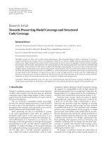
Figure 3: Two-stage CENS feature design (wl = window length, ov = overlap , sr = sampling rate, ds = downsampling factor).
complex orchestral pieces. Our proposed structure analy-
sis algorithm follows the four-stage strategy as described in
Section 1.1. Here, one essential idea is that we account for

musical variations by incorporating invariance and robust-
ness at all four stages simultaneously. The following overview
summarizes the main contributions and describes the struc-
ture of this paper.
(1) Audio features
We introduce a new class of robust and scalable audio fea-
tures considering short-time statistics over chroma-based
energy distributions (Section 2). Such features not only al-
low to absorb variations in parameters such as dynamics,
timbre, articulation, execution of note groups, and tempo-
ral microdeviations, but can also be efficiently processed in
the subsequent steps due to their low resolution. The pro-
posed features s trongly correlate to the short-time harmonic
content of the underlying audio signal.
(2) Similarity measure
As a second contribution, we significantly enhance the path
structure of a self-similarity matrix by incorporating contex-
tual information at various tempo levels into the local simi-
larity measure (Section 3). This accounts for local temporal
variations and significantly smooths the path st ructures.
(3) Path extraction
Based on the enhanced matrix, we suggest a robust and
efficient path extraction procedure using a greedy strategy
(Section 4). This step takes care of relative di fferences in the
tempo progression between musically similar segments.
(4) Global structure
Each path encodes a pair of musically similar segments. To
determine the global repetitive structure, we describe a one-
step transitivity clustering procedure which balances out the
inconsistencies introduced by inaccurate and incorrect path

extractions (Section 5).
We evaluated our structure extraction algorithm on a
wide range of Western classical music including complex or-
chestral and vocal works (Section 6). The experimental re-
sults show that our method successfully identifies the repeti-
tive structure—often corresponding to the musical form of
the underlying piece—even in the presence of significant
variations as indicated by the Brahms and Shostakovich ex-
amples. Our MATLAB implementation performs the struc-
ture analysis task within a couple of minutes even for long
and versatile audio recordings such as Ravel’s Bolero, which
has a duration of more than 15 minutes and possesses a
rich path structure. Further results and an audio demon-
stration can be found at />projects/audiostructure.
2. ROBUST AUDIO FEATURES
In this section, we consider the desig n of audio features,
where one has to deal with two mutually conflicting goals: ro-
bustness to admissible var iations on the one hand and accu-
racy with respect to the relevant characteristics on the other
hand. Furthermore, the features should support an efficient
algorithmic solution of the problem they are designed for. In
our structure analysis scenario, we consider audio segments
as similar if they represent the same musical content regard-
less of the specific articulation and instrumentation. In other
words, the structure extraction procedure has to be robust
to variations in timbre, dynamics, articulation, local tempo
changes, and global tempo up to the point of variations in
note groups such as trills or grace notes.
In this section, we introduce a new class of audio features,
which possess a high degree of robustness to variations of the

above-mentioned parameters and st rongly correlate to the
harmonics information contained in the audio signals. In the
feature extraction, we proceed in two stages as indicated by
Figure 3. In the first stage, we use a small analysis window to
investigate how the signal’s energy locally distr ibutes among
the 12 chroma classes (Section 2.1 ). Using chroma distribu-
tions not only takes into account the close octave relation-
ship in both melody and harmony as prominent in Western
music, see [1], but also introduces a high degree of robust-
ness to variations in dynamics, timbre, and articulation. In
the second stage, we use a much larger statistics window to
compute thresholded short-time statistics over these chroma
energy distributions in order to introduce robustness to lo-
cal time deviations and additional notes ( Section 2.2). (As a
general strategy, statistics such as pitch histograms for audio
signalshavebeenproventobeausefultoolinmusicgenre
classification, see, e.g., [16].) In the following, we identify the
musical notes A0toC8 (the range of a standard piano) with
the MIDI pitches p
= 21 to p = 108. For example, we speak
of the note A4 (frequency 440 Hz) and simply write p
= 69.
M. M
¨
uller and F. Kurth 5
20
0
20
40
60

dB
60 70 80 88–92
Normalized frequency (xπ rad/samples)
0
0.10.20.30.40.50.60.70.80.9
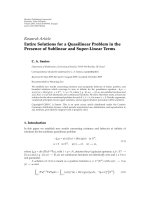
Figure 4: Magnitude responses in dB for the elliptic filters corre-
sponding to the MIDI notes 60, 70, 80, and 88 to 92 with respect to
the sampling rate of 4410 Hz.
2.1. First stage: local chroma energy distribution
First, we decompose the audio signal into 88 frequency bands
with center frequencies corresponding to the MIDI pitches
p
= 21 to p = 108. To properly separate adjacent pitches,
we need filters with narrow passbands, high rejection in the
stopbands, and sharp cutoffs. In order to design a set of fil-
ters satisfying these stringent requirements for all MIDI notes
in question, we work with three different sampling r ates:
22050 Hz for high frequencies (p
= 96, , 108), 4410 Hz for
medium frequencies (p
= 60, , 95), and 882 Hz for low
frequencies (p
= 21, , 59). To this end, the original audio
signal is downsampled to the required sampling rates after
applying suitable antialiasing filters. Working with different
sampling rates also takes into account that the time resolu-
tion naturally decreases in the analysis of lower frequencies.
Each of the 88 filters is realized as an eighth-order elliptic
filter with 1 dB passband ripple and 50 dB reject ion in the
stopband. To separate the notes, we use a Q factor (ratio of

center frequency to bandwidth) of Q
= 25 and a transition
band having half the width of the passband. Figure 4 shows
the magnitude response of some of these filters.
Elliptic filters have excellent cutoff properties as well as
low filter orders. However, these properties are at the expense
of large-phase distortions and group delays. Since in our off-
line scenario the entire audio signals are known prior to the
filtering step, one can apply the following trick: after filtering
in the forward direction, the filtered signal is reversed and
run back through the filter. The resulting output signal has
precisely zero-phase distortion and a magnitude modified by
the square of the filter’s magnitude response. Further details
may be found in standard text books on digital signal pro-
cessing such as [17].
As a next step, we compute the short-time mean-square
power (STMSP) for each of the 88 subbands by convolving
the squared subband signals by a 200 ms rectangular win-
dow with an overlap of half the window size. Note that the
actual window size depends on the respective sampling rate
of 22050, 4410, and 882 Hz, which is compensated in the
energy computation by introducing an additional factor of
1, 5, and 25, respectively. Then, we compute STMSPs of all
chroma classes C, C
#
, , B by adding up the correspond-
ing STMSPs of all pitches belonging to the respective class.
For example, to compute the STMSP of the chroma C,we
add up the STMSPs of the pitches C1, C2, , C8(MIDI
pitches 24, 36, , 108). This yields for every 100 ms a real

12-dimensional vector

v
= ( v
1
, v
2
, v
12
) ∈ R
12
,wherev
1
corresponds to chroma C, v
2
to chroma C
#
, and so on. Fi-
nally, we compute the energy distribution relative to the 12
chroma classes by replacing

v by

v/(

12
i
=1
v
i

).
In summary, in the first stage the audio signal is con-
verted into a sequence (

v
1
,

v
2
, ,

v
N
) of 12-dimensional
chroma distribution vectors

v
n
∈ [0, 1]
12
for 1 ≤ n ≤ N.
For the Brahms example given in the introduction, the result-
ing sequence is shown in Figure 5 (light curve). Furthermore,
to avoid random energy distributions occurring during pas-
sages of very low energy (e.g., passages of silence before the
actual start of the recording or during long pauses), we as-
sign an equally distributed chroma energy to such passages.
We also tested the short-time Fourier transform (STFT) to
compute the chroma features by pooling the spectral coef-

ficients as suggested in [1]. Even though obtaining similar
features, our filter bank approach, while having a compara-
ble computational cost, al lows a better control over the fre-
quency bands. This particularly holds for the low frequen-
cies, which is due to the more adequate resolution in time
and frequency.
2.2. Second stage: normalized short-time statistics
In view of possible v ariations in local tempo, articulation,
and note execution, the local chroma energy distribution fea-
tures are still too sensitive. Furthermore, as it will turn out
in Section 3, a flexible and computationally inexpensive pro-
cedure is needed to adjust the feature resolution. Therefore,
we further process the chroma features by introducing a sec-
ond much larger statistics window and consider short-time
statistics concerning the chroma energy distribution over this
window. More s pecifically, let Q : [0, 1]
→{0, 1,2, 3, 4} be a
quantization function defined by
Q(a):
=
⎧
⎪
⎪
⎪
⎪
⎪
⎪
⎪
⎪
⎪

⎪
⎪
⎪
⎨
⎪
⎪
⎪
⎪
⎪
⎪
⎪
⎪
⎪
⎪
⎪
⎪
⎩
0for0≤ a<0.05,
1for0.05
≤ a<0.1,
2for0.1
≤ a<0.2,
3for0.2
≤ a<0.4,
4for0.4
≤ a ≤ 1.
(1)
Then, we quantize each chroma energy distribution vec-
tor


v
n
= (v
n
1
, , v
n
12
) ∈ [0, 1]
12
by applying Q to each com-
ponent of

v
n
, yielding Q(

v
n
):= (Q(v
n
1
), , Q(v
n
12
)). Intu-
itively, this quantization assigns a value of 4 to a chroma
component v
n
i

if the corresponding chroma class contains
more than 40 percent of the signal’s total energy and so
on. The thresholds are chosen in a logarithmic fashion. Fur-
thermore, chroma components below a 5-percent threshold
are excluded from further considerations. For example, the
vector

v
n
= (0.02, 0.5, 0.3, 0.07, 0.11, 0, ,0)istransformed
into the vector Q(

v
n
):= (0,4,3,1,2,0, ,0).
In a subsequent step, we convolve the sequence (Q(

v
1
),
, Q(

v
N
)) componentwise with a Hann window of length
w
∈ N. This again results in a sequence of 12-dimensional
vectors with nonnegative entries, representing a kind of
6 EURASIP Journal on Advances in Sig nal Processing
B

A#
A
G#
G
F#
F
E
D#
D
C#
C
0
1
0
1
0
1
0
1
0
1
0
1
0
1
0
1
0
1
0

1
0
1
0
1
0 5 10 15 20 25
(a)
B
A#
A
G#
G
F#
F
E
D#
D
C#
C
0
1
0
1
0
1
0
1
0
1
0

1
0
1
0
1
0
1
0
1
0
1
0
1
0 2 4 6 8 10 12 14 16 18 20
(b)
Figure 5: Local chroma energy distributions (light curves, 10 feature vectors per second) and CENS feature sequence (dark bars, 1 feature
vector per second) of the segment [42 : 69] ((a) corresponding to B
1
) and segment [69 : 89] ((b) corresponding to B
2
) of the Brahms example
shown in Figure 1. Note that even though the relative tempo progression in the parts B
1
and B
2
is different, the harmonic progression at the
low resolution level of the CENS features is very similar.
weighted statistics of the energy distribution over a window
of w consecutive vectors. In a last step, this sequence is down-
sampled by a factor of q. The resulting vectors are normalized

with respect to the Euclidean norm. For example, if w
= 41
and q
= 10, one obtains one feature vector per second, each
corresponding to roughly 4100 ms of audio. For short, the
resulting features are referred to as CENS[w, q](chromaen-
ergy distribution normalized statistics). These features are el-
ements of the following set of vectors:
F :
=


v
=

v
1
, , v
12


∈ [0, 1]
12
|
12

i=1
v
2
i

= 1

. (2)
Figure 5 shows the resulting sequence of CENS feature vec-
tors for our Brahms example. Similar features have been ap-
plied in the audio matching scenar io; see [18].
By modifying the parameters w and q,wemayadjust
the feature granularity and sampling rate without repeating
the cost-intensive computations in Section 2.1. Furthermore,
changing the thresholds and values of the quantization func-
tion Q allows to enhance or mask out certain aspects of the
audio signal, for example, making the CENS features insensi-
tive to noise components that may arise during note attacks.
Finally, using statistics over relatively large windows not only
smooths out microtemporal deviations, as may occur for ar-
ticulatory reasons, but also compensates for different realiza-
tionsofnotegroupssuchastrillsorarpeggios.
In conclusion, we mention some potential problems con-
cerning the proposed CENS features. The usage of a filter
bank with fixed frequency bands is based on the assump-
tion of well-tuned instruments. Slight deviations of up to
30–40 cents from the center frequencies can be compensated
by the filters which have relatively wide passbands of con-
stant amplitude response. Global deviations in tuning can
be compensated by employing a suitably adjusted filter bank.
However, phenomena such as strong string vibratos or pitch
oscillation as is typical for, for example, kettledrums lead to
significant and problematic pitch smearing effects. Here, the
detection and smoothing of such fluctuations, which is cer-
tainly not an easy task, may be necessary prior to the filtering

step. However, as we will see in Section 6, the CENS features
generally still lead to good analysis results even in the pres-
ence of the artifacts mentioned above.
3. SIMILARITY MEASURE
In this section, we introduce a strategy for enhancing the
path structure of a self-similarity matrix by designing a suit-
able local similarity measure. To this end, we proceed in three
steps. As a starting point, let d : F
× F → [0, 1] be the simi-
larity measure on the space F
⊂ R
12
of CENS feature vectors
(see (2)) defined by
d(

v,

w):
= 1 −

v,

w
 (3)
for CENS[w, q]-vectors

v,

w

∈ F . Since

v and

w are normal-
ized, the inner product


v,

w
 coincides with the cosine of the
angle between

v and

w. For short, the resulting self-similarity
matrix wil l also be denoted by S[w, q] or simply by S if w and
q are clear from the context.
To further enhance the path structure of S[w, q], we in-
corporate contextual information into the local similarity
measure. A similar approach has been suggested in [1]or[5],
where the self-similar ity matrix is filtered along diagonals as-
suming constant tempo. We will show later in this section
how to remove this assumption by, intuitively speaking, fil-
tering along various directions simultaneously, where each of
the directions corresponds to a different local tempo. In [7],
M. M
¨
uller and F. Kurth 7

220
200
180
160
140
120
100
80
60
40
20
50 100 150 200
(a)
210
200
190
180
170
160
150
140
10 20 30 40
(b)
220
200
180
160
140
120
100

80
60
40
20
50 100 150 200
(c)
210
200
190
180
170
160
150
140
10 20 30 40
(d)
220
200
180
160
140
120
100
80
60
40
20
50 100 150 200
(e)
210

200
190
180
170
160
150
140
10 20 30 40
(f)
Figure 6: Enhancement of the similarity matrix of the Shostakovich
example; see Figure 2. (a) and (b): S[41, 10] and enlargement. (c)
and (d): S
10
[41, 10] and enlargement. (e) and (f): S
min
10
[41, 10] and
enlargement.
matrix enhancement is achieved by using HMM-based “dy-
namic” features, which model the temporal evolution of the
spectral shape over a fixed time duration. For the moment,
we also assume constant tempo and then, in a second step,
describe how to get rid of this assumption. Let L
∈ N be a
length parameter. We define the contextual similarity measure
d
L
by
d
L

(n, m):=
1
L
L−1

=0
d


v
n+
,

v
m+

,(4)
where 1
≤ n, m ≤ N − L +1. By suitably extending the CENS
sequence (

v
1
, ,

v
N
), for example, via zero-padding, one
may extend the definition to 1
≤ n, m ≤ N. Then, the contex-

tual similarity matrix S
L
is defined by S
L
(n, m):= d
L
(n, m).
In this matrix, a value d
L
(n, m) ∈ [0, 1] close to zero im-
plies that the entire L-sequence (

v
n
, ,

v
n+L−1
) is similar
to the L-sequence (

v
m
, ,

v
m+L−1
), resulting in an enhance-
ment of the diagonal path structure in the similarity matrix.
Table 1: Tempo changes (tc) simulated by changing the statistics

window size w and the downsampling factor q.
w 29 33 37 41 45 49 53 57
q 78910 11 12 13 14
tc 1.43 1.25 1.1 1.0 0.9 0.83 0.77 0.7
This is also illustrated by our Shostakovich example, showing
S[41, 10] in Figure 6(a) and S
10
[41, 10] in Figure 6(c).Here,
the diagonal path structure of S
10
[41, 10]—as opposed to the
one of S[41, 10]—is much clearer, which not only facilitates
the extraction of structural information but also allows to
further decrease the feature sampling rate. Note that the con-
textual similarity mat rix S
L
can be efficiently computed from
S by applying an averaging filter along the diagonals. More
precisely, S
L
(n, m) = (1/L)

L−1

=0
S(n + , m + ) (with a suit-
able zero-padding of S).
So far, we have enhanced similarity matrices by regard-
ing the context of L consecutive features vectors. This proce-
dure is problematic when similar segments do not have the

same tempo. Such a situation frequently occurs in classical
music—even within the same interpretation—as is shown
by our Brahms example; see Figure 1.Toaccountforsuch
variations we, intuitively speaking, create several versions of
one of the audio data streams, each corresponding to a dif-
ferent global tempo, which are then incorporated into one
single similarity measure. More precisely, let

V[w, q]denote
the CENS[w, q] sequence of length N[w, q] obtained from
the audio data stream in question. For the sake of concrete-
ness, we choose w
= 41 and q = 10 as reference parameters,
resulting in a feature sampling rate of 1 Hz. We now simulate
a tempo change of the data stream by modifying the values
of w and q. For example, using a window size of w
= 53 (in-
stead of 41) and a downsampling factor of q
= 13 (instead
of 10) simulates a tempo change of the original data stream
by a factor of 10/13
≈ 0.77. In our experiments, we used 8
different tempi as indicated by Ta bl e 1, covering tempo vari-
ations of roughly
−30 to +40 percent. We then define a new
similarity measure d
min
L
by
d

min
L
(n, m):= min
[w,q]
1
L
L−1

=0
d


v[41, 10]
n+
,

v[w, q]
m+

,(5)
where the minimum is taken over the pairs [w, q]listed
in Table 1 and
m =m · 10/q.Inotherwords,atposi-
tion (n, m), the L-subsequence of

V[41, 10] starting at ab-
solute time n (note that the feature sampling rate is 1 Hz)
is compared with the L-subsequence of

V[w, q] (simulating

atempochangeof10/q) starting at absolute time m (cor-
responding to feature position m =m · 10/q). From this
we obtain the modified contextual similarity matrix S
min
L
de-
fined by S
min
L
(n, m):= d
min
L
(n, m). Figure 7 shows that in-
corporating local tempo variations into contextual similarity
matrices significantly improves the quality of the path struc-
ture, in particular for the case that similar audio segments
exhibit different local relative tempi.
8 EURASIP Journal on Advances in Sig nal Processing
200
180
160
140
120
100
80
60
40
20
50 100 150 200
(a)

100
90
80
70
60
50
40
40 50 60 70 80 90 100
(b)
200
180
160
140
120
100
80
60
40
20
50 100 150 200
(c)
100
90
80
70
60
50
40
40 50 60 70 80 90 100
(d)

200
180
160
140
120
100
80
60
40
20
50 100 150 200
(e)
100
90
80
70
60
50
40
40 50 60 70 80 90 100
(f)
Figure 7: Enhancement of the similarity matrix of the Brahms ex-
ample; see Figure 1. (a) and (b): S[41, 10] and enlargement. (c) and
(d): S
10
[41, 10] and enlargement. (e) and (f): S
min
10
[41, 10] and en-
largement.

4. PATH EXTRACTION
In the last two sections, we have introduced a combination of
techniques—robust CENS features and usage of contextual
information—resulting in smooth and structurally enhanced
self-similarity matrices. We now describe a flexible and effi-
cient strategy to extract the paths of a given self-similarity
matrix S
= S
min
L
[w, q].
Mathematically, we define a path to be a sequence P
=
(p
1
, p
2
, , p
K
) of pairs of indices p
k
= (n
k
, m
k
) ∈ [1 : N]
2
,
1
≤ k ≤ K, satisfying the path constraints

p
k+1
= p
k
+ δ for some δ ∈ Δ,(6)
where Δ :
={(1, 1), (1, 2), (2, 1)} and 1 ≤ k ≤ K − 1. The
pairs p
k
will also be called the links of P. Then the cost of link
p
k
= (n
k
, m
k
)isdefinedasS(n
k
, m
k
). Now, it is the objective
to extract long paths consisting of links having low costs. Our
path extraction algorithm consists of three steps. In step (1),
we start with a link of minimal cost, referred to as initial link,
and construct a path in a greedy fashion by iteratively adding
links of low cost, referred to as admissible links.Instep(2),all
links in a neighborhood of the construc ted path are excluded
from further considerations by suitably modifying S.Then,
steps (1) and (2) are repeated until there are no links of low
cost left. Finally, the extracted paths are postprocessed in step

(3). The details are as fol lows.
(0) Initialization
Set S
= S
min
L
[w, q] and let C
in
, C
ad
∈ R
>0
be two suitable
thresholds for the maximal cost of the initial links and the
admissible links, respectively. (In our experiments, we typi-
cally chose 0.08
≤ C
in
≤ 0.15 and 0.12 ≤ C
ad
≤ 0.2.) We
modify S by setting S(n, m)
= C
ad
for n ≤ m, that is, the
links below the diagonal will be excluded in the following
steps. Similarly, we exclude the neighborhood of the diago-
nal path P
= ((1, 1), (2, 2), ,(N, N)) by modifying S using
the path removal strategy as described in step (2).

(1) Path construction
Let p
0
= (n
0
, m
0
) ∈ [1 : N]
2
be the indices minimizing
S(n, m). If S(n
0
, m
0
) ≥ C
in
, the algorithm terminates. Oth-
erwise, we construct a new path P by extending p
0
iteratively,
where all possible extensions are described by Figure 8(a).
SupposewehavealreadyconstructedP
= (p
a
, , p
0
, , p
b
)
for a

≤ 0andb ≥ 0. Then, if min
δ∈Δ
(S(p
b
+ δ)) <C
ad
,we
extend P by setting
p
b+1
:= p
b
+argmin
δ∈Δ

S

p
b
+ δ

,(7)
and if min
δ∈Δ
(S(p
a
− δ)) <C
ad
,extendP by setting
p

a−1
:= p
a
− arg min
δ∈Δ

S

p
a
− δ

. (8)
Figure 8(b) illustr ates such a path. If there are no further
extensions with admissible links, we proceed with step (2).
Shifting the indices by a + 1, we may assume that the result-
ing path is of the form P
= (p
1
, , p
K
)withK = a + b +1.
(2) Path removal
For a fixed link p
k
= (n
k
, m
k
)ofP, we consider the maximal

number m
k
≤ m
∗
≤ N with the property that S(n
k
, m
k
) ≤
S(n
k
, m
k
+1) ≤ ··· ≤ S(n
k
, m
∗
). In other words, the se-
quence (n
k
, m
k
), (n
k
, m
k
+1), ,(n
k
, m
∗

)definesaray start-
ing at position (n
k
, m
k
) and running horizontally to the right
such that S is monotonically increasing. Analogously, we
consider three other types of rays starting at position (n
k
, m
k
)
running horizontally to the left, vertically upwards, and verti-
cally downwards; see Figure 8(c) for an illustration. We then
consider all such rays for all links p
k
of P.LetN (P) ⊂ [1 :
N]
2
be the set of all pairs (n, m) lying on one of these rays.
Note that N (P) defines a neighborhood of the path P.Toex-
clude the links of N (P) from further consideration, we set
S(n, m)
= C
ad
for all (n, m) ∈ N (P) and continue by repeat-
ing step (1).
M. M
¨
uller and F. Kurth 9

(a) (b)
(c)
Figure 8: (a) Initial link and possible path extensions. (b) Path re-
sulting from step (1). (c) Rays used for path removal in step (2).
In our actual implementation, we made step (2) more ro-
bust by softening the monotonicity condition on the rays.
After the above algorithm terminates, we obtain a set of
paths denoted by P , which is postprocessed in a third step
by means of some heuristics. For the following, let P
=
(p
1
, p
2
, , p
K
) denote a path in P .
(3a) Removing short paths
All paths that have a length K shorter than a threshold K
0
∈
N
are removed. (In our experiments, we chose 5 ≤ K
0
≤ 10.)
Such paths frequently occur as a result of residual links that
have not been correctly removed by step (2).
(3b) Pruning paths
We prune e ach pa th P
∈ P at the beginning by removing

the links p
1
, p
2
, , p
k
0
up to the index 0 ≤ k
0
≤ K,where
k
0
denotes the maximal index such that the cost of each link
p
1
, p
2
, , p
k
0
exceeds some suitably chosen threshold C
pr
ly-
ing in between C
in
and C
ad
. Analogously, we prune the end
of each path. This step is performed due to the following ob-
servation: introducing contextual information into the local

similarity measure results in a smoothing effect of the paths
along the diagonal direction. This, in turn, results in a blur-
ring effect at the beg inning and end of such paths—as illus-
trated by Figure 6(f)—unnaturally extending such paths at
both ends in the construction of step (1).
(3c) Extending paths
We then extend each path P
∈ P at its end by adding
suitable links p
K+1
, , p
K+L
0
. This step is performed due
to the following reason: since we have incorporated contex-
tual information into the local similarit y measure, a low cost
S(p
K
) = d
min
L
(n
K
, m
K
) of the link p
K
= (n
K
, m

K
)implies
200
150
100
50
50 100 150 200
0.15
0.1
0.05
0
(a)
200
150
100
50
50 100
150
200
(b)
200
150
100
50
50 100 150 200
(c)
200
150
100
50

2
7
1
4
3
6
5
50 100 150 200
(d)
Figure 9: Illustration of the path extraction algorithm for the
Brahms example of Figure 1. (a) Self-similarity matrix S
=
S
min
16
[41, 10]. Here, all values exceeding the threshold C
ad
= 0.16 are
plotted in white. (b) Matrix S after step (0) (initialization). (c) Ma-
trix S after performing steps (1) and (2) once using the thresholds
C
in
= 0.08 and C
ad
= 0.16. Note that a long path in the left upper
corner was constructed, the neighborhood of which has then been
removed. (d) Resulting path set P
={P
1
, , P

7
} after the postpro-
cessing of step (3) using K
0
= 5andC
pr
= 0.10. The index m of P
m
is indicated along each respective path.
that the whole sequence (

v
n
K
[41, 10], ,

v
n
K
+L−1
[41, 10]) is
similar to (

v
m
K
[w, q], ,

v
m

K
+L−1
[w, q]) for the minimizing
[w, q]ofTable 1;seeSection 3. Here the length and direc-
tion of the extension p
K+1
, , p
K+L
0
depends on the values
[w, q]. (In the case [w, q]
= [41, 10], we set L
0
= L and
p
k
= p
K
+(k, k)fork = 1, , L
0
.)
Figure 9 illustrates the steps of our path extraction algo-
rithm for the Br ahms example. Part (d) shows the result-
ing path set P . Note that each path corresponds to a pair
of similar segments and encodes the relative tempo progres-
sion between these two segments. Figure 10(b) shows the set
P for the Shostakovich example. In spite of the matrix en-
hancement, the similarity between the segments correspond-
ing to A
1

and A
3
has not been correctly identified, resulting
in the aborted path P
1
(which should correctly start at link
(4, 145)). Even though, as we will show in the next section,
the extracted information is sufficient to correctly derive the
global structure.
5. GLOBAL STRUCTURE ANALYSIS
In this section, we propose an algorithm to determine the
global repetitive structure of the underlying piece of music
from the relations defined by the extracted paths. We first
introduce some notation. A segment α
= [s : t]isgivenby
its starting point s and end point t,wheres and t are given
10 EURASIP Journal on Advances in Sig nal Processing
200
150
100
50
50 100 150 200
0.15
0.1
0.05
0
(a)
200
150
100

50
3
1
6
2
5
4
50 100 150 200
(b)
Figure 10: Shostakovich example of Figure 2.(a)S
min
16
[41, 10]. (b)
P
={P
1
, , P
6
} based on the same parameters as in the Brahms
example of Figure 9. The index m of P
m
is indicated along each re-
spective path.
in terms of the corresponding indices in the feature sequence

V
= (

v
1

,

v
2
, ,

v
N
); see Section 1.Asimilarity cluster A :=
{
α
1
, , α
M
} of size M ∈ N is defined to be a set of segments
α
m
,1≤ m ≤ M, which are considered to be mutually similar.
Then, the g lobal structure is described by a complete list of
relevant similarity clusters of maximal size.
In other words, the list should represent all repetitions
of musically relevant segments. Furthermore, if a cluster
contains a segment α, then the cluster should also con-
tain all other segments similar to α. For example, in our
Shostakovich example of Figure 2 the global structure is de-
scribed by the clusters A
1
={α
1
, α

2
, α
3
, α
4
} and A
2
=
{
γ
1
, γ
2
}, where the segments α
k
correspond to the parts A
k
for 1 ≤ k ≤ 4 and the segments γ
k
to the parts C
k
for 1 ≤
k ≤ 2. Given a cluster A ={α
1
, , α
M
} with α
m
= [s
m

: t
m
],
1
≤ m ≤ M, the support of A is defined to be the subset
supp(A):
=
M

m=1

s
m
: t
m

⊂ [1 : N] . (9)
Recall that each path P indicates a pair of similar seg-
ments. More precisely, the path P
= (p
1
, , p
K
)withp
k
=
(n
k
, m
k

) indicates that the segment π
1
(P):= [n
1
: n
K
]is
similar to the segment π
2
(P):= [m
1
: m
K
]. Such a pair
of segments will also be referred to as a path relation.As
an example, Figure 11(a) shows the path relations of our
Shostakovich example. In this section, we describe an al-
gorithm that derives large and consistent similarity clusters
from the path relations induced by the set P of extracted
paths. From a theoretical point of view, one has to construct
some kind of transitive closure of the path relations; see also
[3]. For example, if segment α is similar to segment β,and
segment β is similar to segment γ, then α should also be re-
garded as similar to γ resulting in the cluster
{α, β, γ}.The
situation becomes more complicated when α overlaps with
some segment β which, in turn, is similar to seg ment γ. This
would imply that a subsegment of α is similar to some sub-
segment of γ. In practice, the construction of similarity clus-
ters by iteratively continuing in the above fashion is prob-

lematic. Here, inconsistencies in the path relations due to se-
mantic (vague concept of musical similarity) or algorithmic
2
4
6
20 40 60 80 100 120 140 160 180 200 220
(a)
2
4
6
8
10
12
20 40 60 80 100 120 140 160 180 200 220
(b)
2
4
6
20 40 60 80 100 120 140 160 180 200 220
(c)
1
2
20 40 60 80 100 120 140 160 180 200 220
(d)
Figure 11: Illustration of the clustering algorithm for the
Shostakovich example. The path set P
={P
1
, , P
6

} is shown
in Figure 10(b). S egments are indicated by gray bars and overlaps
are indicated by black regions. (a) Illustration of the two segments
π
1
(P
m
)andπ
2
(P
m
)foreachpathP
m
∈ P ,1 ≤ m ≤ 6. Row m
corresponds to P
m
. (b) Clusters A
1
m
and A
2
m
(rows 2m − 1 and 2m)
computed in step (1) with T
ts
= 90. (c) Clusters A
m
(row m)com-
puted in step (2). (d) Final result of the clustering algorithm after
performing step (3) with T

dc
= 90. The derived global structure is
given by two similarity clusters. The first cluster corresponds to the
musical parts
{A
1
, A
2
, A
3
, A
4
} (first row) and the second cluster to
{C
1
, C
2
} (second row) (cf. Figure 2).
(inaccurately extracted or missing paths) reasons may lead to
meaningless clusters, for example, containing a series of seg-
ments where each segment is a slightly shifted version of its
predecessor. For example, let α
= [1 : 10], β = [11 : 20],
γ
= [22 : 31], and δ = [3 : 11]. Then similarity relations
between α and β, β and γ,andγ and δ would imply that
α
= [1:10]hastoberegardedassimilartoδ = [3 : 11], and
so on. To balance out such inconsistencies, previous strate-
gies such as [4] rely upon the constant tempo assumption. To

achieve a robust and meaningful clustering even in the pres-
ence of significant local tempo variations, we suggest a new
clustering algorithm, which proceeds in three steps. To this
end, let P
={P
1
, P
2
, , P
M
} be the set of extracted paths
M. M
¨
uller and F. Kurth 11
P
m
,1≤ m ≤ M. In step (1) (transitivity step) and step (2)
(merging step), we compute for each P
m
a similar ity clus-
ter A
m
consisting of all segments that are either similar to
π
1
(P
m
)ortoπ
2
(P

m
). In step (3), we then discard the redun-
dant clusters. We exemplarily explain the procedure of steps
(1) and (2) by considering the path P
1
.
(1) Transitivity step
Let T
ts
be a suitable tolerance parameter measured in percent
(in our experiments we used T
ts
= 90). First, we construct a
cluster A
1
1
for the path P
1
and the segment α := π
1
(P
1
). To
this end, we check for all paths P
m
whether the intersection
α
0
:= α ∩ π
1

(P
m
) contains more than T
ts
percent of α, that is,
whether
|α
0
|/|α|≥T
ts
/100. In the affirmative case, let β
0
be
the subsegment of π
2
(P
m
) that corresponds under P
m
to the
subsegment α
0
of π
1
(P
m
). We add α
0
and β
0

to A
1
1
. Similarly,
we check for all paths P
m
whether the intersection α
0
:= α ∩
π
2
(P
m
) contains more than T
ts
percent of α and add in the
affirmative case α
0
and β
0
to A
1
1
, where this time β
0
is the
subsegment of π
1
(P
m

) that corresponds under P
m
to α
0
.Note
that β
0
generally does not have the same length as α
0
.(Recall
that the relative tempo v ariation is encoded by the gradient
of P
m
.) Analogously, we construct a cluster A
2
1
for the path
P
1
and the segment α := π
2
(P
1
). The clusters A
1
1
and A
2
1
can be regarded as the result of the first iterative step towards

forming the transitive closure.
(2) Merging step
The cluster A
1
is constructed by basically merging the clus-
ters A
1
1
and A
2
1
. To this end, we compare each segment
α
∈ A
1
1
with each segment β ∈ A
2
1
. In the case that the
intersection γ :
= α ∩ β contains more than T
ts
percent of
α and of β (i.e., α essentially coincides with β), we add the
segment γ to A
1
. In the case that for a fixed α ∈ A
1
1

the
intersection α
∩ supp(A
2
1
) contains less than (100 − T
ts
)per-
cent of α (i.e., α is essentially disjoint with all β
∈ A
2
1
), we
add α to A
1
. Symmetrically, if for a fixed β ∈ A
2
1
the inter-
section β
∩ supp(A
1
1
) contains less than (100 − T
ts
)percent
of β,weaddβ to A
1
. Note that by this procedure, the first
case balances out small inconsistencies, whereas the second

case and the third case compensate for missing path relations.
Furthermore, segments α
∈ A
1
1
and β ∈ A
2
1
that do not fall
into one of the above categories indicate significant inconsis-
tencies and are left u nconsidered in the construction of A
1
.
After steps (1) and (2), we obtain a cluster A
1
for the path
P
1
. In an a nalogous fashion, we compute clusters A
m
for all
paths P
m
,1≤ m ≤ M.
(3) Discarding clusters
Let T
dc
be a suitable tolerance parameter measured in per-
cent (in our experiments we chose T
dc

between80and90
percent). We say that cluster A is a T
dc
-cover of cluster B if
the intersection supp(A)
∩ supp(B) contains more than T
dc
percent of supp(B). By pairwise comparison of all clusters
A
m
, we successively discard all clusters that are T
dc
-covered
2
4
6
20 40 60 80 100 120 140 160 180 200
(a)
2
4
6
8
10
12
14
20 40 60 80 100 120 140 160 180 200
(b)
2
4
6

20 40 60 80 100 120 140 160 180 200
(c)
1
2
3
20 40 60 80 100 120 140 160 180 200
(d)
Figure 12: Steps of the clustering algorithm for the Brahms exam-
ple, see Figure 9.FordetailswerefertoFigure 11. The final result
correctly represents the global structure: the cluster of the second
row corresponds to
{B
1
, B
2
, B
3
, B
4
}, and the one of the third row to
{A
1
, A
2
, A
3
}. Finally, the cluster of the first row expresses the simi-
larity between A
2
B

1
B
2
and A
3
B
3
B
4
(cf. Figure 1).
by some other cluster consisting of a larger number of seg-
ments. (Here the idea is that a cluster with a larger number
of smaller segments contains more information than a cluster
having the same support while consisting of a smaller num-
ber of larger segments.) In the case that two clusters are mu-
tual T
dc
-covers and consist of the same number of segments,
we discard the cluster with the smaller support.
The steps of the clustering algorithm are a lso illustrated
by Figures 11 and 12.RecallfromSection 4 that in the
Shostakovich example, the significant variations in the in-
strumentation led to a defective path extraction. In par tic-
ular, the similar ity of the segments corresponding to parts
A
1
and A
3
could not be correctly identified as reflected by
the truncated path P

1
; see Figures 10(b) and 11(a).Never-
theless, the correct global str ucture was derived by the clus-
tering algorithm (cf. Figure 11(d)). Here, the missing rela-
tion was recovered by step (1) (transitivity step) from the
12 EURASIP Journal on Advances in Sig nal Processing
150
100
50
50 100 150
0.15
0.1
0.05
0
1
2
50 100 150
(a)
300
250
200
150
100
50
100 200 300
0.15
0.1
0.05
0
1

3
50 100 150 200 250 300
(b)
200
150
100
50
50 100 150 200
0.15
0.1
0.05
0
0.5
1.5
50 100 150 200
(c)
250
200
150
100
50
50 150 250
0.15
0.1
0.05
0
1
2
50 100 150 200 250
(d)

Figure 13: (a) Chopin, “Tristesse,” Etude op. 10/3, played by Varsi. (b) Beethoven, “Pathetique,” second movement, op. 13, played by Baren-
boim. (c) Gloria Gaynor, “I will survive.” (d) Part A
1
A
2
B of the Shostakovich example of Figure 2 repeated three times in modified tempi
(normal tempo, 140 percent of normal tempo, accelerating tempo from 100 to 140 percent).
correctly identified similarit y relation between segments cor-
responding to A
3
and A
4
(path P
2
) and between segments
corresponding to A
1
and A
4
(path P
3
). The effectofstep(3)
is illustrated by comparing (c) and (d) of Figure 11. Since the
cluster A
5
is a 90-percent cover of the clusters A
1
, A
2
, A

3
,
and A
6
, and has the largest support, the latter clusters are
discarded.
6. EXPERIMENTS
We implemented our algorithm for audio structure analy-
sis in MATLAB and tested it on about 100 audio record-
ings reflecting a wide range of mainly Western classical mu-
sic, including pieces by Bach, Beethoven, Brahms, Chopin,
Mozart, Ravel, Schubert, Schumann, Shostakovich, and Vi-
valdi. In particular, we used musically complex orchestral
pieces exhibiting a large degree of variations in their repeti-
tions with respect to instrumentation, articulation, and local
tempo variations. From a musical point of view, the global
repetitive structure is often ambiguous since it depends on
the particular notion of similarity, on the degree of admissi-
ble variations, as well as on the musical significance and du-
ration of the respective repetitions. Furthermore, the struc-
tural analysis can be performed at v arious levels: at a global
level (e.g., segmenting a sonata into exposition, repetition of
the exposition, development, and recapitulation), an inter-
mediary level (e.g., fur ther splitting up the exposition into
first and second theme), or on a fine level (e.g., segmenting
into repeating motifs). This makes the automatic str ucture
extraction as well as an objective evaluation of the results a
difficult and problematic task.
In our experiments, we looked for repetitions at a
global to intermediary level corresponding to segments of

at least 15–20 seconds of duration, which is reflected in
our choice of parameters; see Section 6.1. In that section,
we will also present some general results and discuss in de-
tail two complex examples: Mendelssohn’s Wedding March
and Ravel’s Bolero. In Section 6.2, we discuss the running
time behavior of our implementation. It turns out that the
algorithm is applicable to pieces even longer than 45 min-
utes, which covers essentially any piece of Western classi-
cal music. To account for transposed (pitch-shifted) repeat-
ing segments, we adopted the shifting technique suggested
by Goto [4]. Some results will be discussed in Section 6.3.
Further results and an audio demonstration can be found at
/>6.1. General Results
In order to demonstra te the capability of our structure anal-
ysis algorithm, we discuss some representative results in de-
tail. This will also illustrate the kind of difficulties generally
found in music structure analysis. Our algorithm is fully au-
tomatic, in other words, no prior knowledge about the re-
spective piece is exploited in the analysis. In all examples,
we use the following fixed set of parameters. For the self-
similarity matrix, we use S
min
16
[41, 10] with a corresponding
feature resolution of 1 Hz; see Section 3. In the path extrac-
tion algorithm of Section 4,wesetC
in
= 0.08, C
ad
= 0.16,

C
pr
= 0.10, and K
0
= 5. Finally, in the clustering algorithm
of Section 5,wesetT
ts
= 90 and T
dc
= 90. The choice of the
above parameters and thresholds constitutes a trade-off be-
tween being tolerant enough to allow relevant var iations and
being robust enough to deal with artifacts and inconsisten-
cies.
As a first example, we consider a Varsi recording of
Chopin’s Etude op. 10/3 “Tristesse.” The underlying piece has
the musical for m A
1
A
2
B
1
CA
3
B
2
D. This structure has suc-
cessfully been extracted by our algor ithm; see Figure 13(a).
Here, the first cluster A
1

corresponds to the parts A
2
B
1
and
A
3
B
2
, whereas the second cluster A
2
corresponds to the parts
A
1
, A
2
,andA
3
. For simplicity, we use the notation A
1
∼
{A
2
B
1
, A
3
B
2
} and A

2
∼ {A
1
, A
2
, A
3
}. The similarity relation
between B
1
and B
2
is induced from cluster A
1
by “subtract-
ing” the respective A-part which is known from cluster A
2
.
The small gaps between the segments in cluster A
2
are due
to the fact that the tail of A
1
(passage to A
2
)isdifferent from
the tail of A
2
(passage to B
1

).
The next example is a Barenboim interpretation of the
second movement of Beethoven’s Pathetique, which has the
M. M
¨
uller and F. Kurth 13
2
4
6
8
50 100 150 200 250 300
(a)
5
10
15
100 200 300 400 500 600 700 800 900
(b)
Figure 14: (a) Mendelssohn, “Wedding March,” op. 21-7, conducted by Tate. (b) Ravel, “Bolero,” conducted by Ozawa.
musical form A
1
A
2
BA
3
CA
4
A
5
D. The interesting point of this
piece is that the A-parts are variations of each other. For ex-

ample, the melody in A
2
and A
4
is played one octave higher
than the melody in A
1
and A
3
. Furthermore, A
3
and A
4
are rhythmic variations of A
1
and A
2
. Nevertheless, the cor-
rect global structure has been extracted; see Figure 13(b).
The three clusters are in correspondence with A
1
∼
{A
1
A
2
, A
4
A
5

}, A
3
∼ {A
1
, A
3
, A
5
},andA
2
∼ {A

1
, A

2
, A

3
,
A

4
, A

5
},whereA

k
denotes a truncated version of A

k
.Hence,
the segments A
1
, A
3
,andA
5
are identified as a whole,
whereas the other A-parts are identified only up to their tail.
This is due to the fact that the tails of the A-parts exhibit
some deviations leading to higher costs in the self-similarity
matrix, as illustrated by Figure 13(b).
The popular song “I will survive” by Gloria Gaynor con-
sists of an introduction I followed by eleven repetitions A
k
,
1
≤ k ≤ 11, of the chorus. This highly repetitive structure
is reflected by the secondar y diagonals in the self-similarity
matrix; see Figure 13(c). The segments exhibit variations not
only with respect to the lyrics but also with respect to instru-
mentation and tempo. For example, some segments include a
secondary voice in the violin, others harp arpeggios, or trum-
pet syncopes. The first chorus A
1
is played without percus-
sion, whereas A
5
is a purely instrumental version. Also note

that there is a significant ritardando in A
9
between seconds
150 and 160. In spite of these variations, the structure analy-
sis algorithm works almost correctly. However, there are two
artifacts that have not been ruled out by our strategy. Each
chorus A
k
can be split up into two subparts A
k
= A

k
A

k
.The
computed cluster A
1
corresponds to the ten parts A

k−1
A

k
A

k
,
2

≤ k ≤ 11, revealing an overlap in the A

-parts. In particu-
lar, the extracted segments are “out of phase” since they start
with subsegments corresponding to the A

-parts. This may
be due to extreme variations in A

1
making this part dissimi-
lar to the other A

-parts. Since A

1
constitutes the beginning
of the extracted paths, it has been (mistakenly) truncated in
step (3b) (pruning paths) of Section 4.
To check the robustness of our algorithm with respect
to global and local tempo variations, we conducted a se-
ries of experiments with synthetically time-stretched au-
dio signals (i.e., we changed the tempo progression with-
out changing the pitch). As it turns out, there are no prob-
lems in identifying similar segments that exhibit global
tempo variations of up to 50 percent as well as local tempo
variations such as ritardandi and accelerandi. As an exam-
ple, we consider the audio file corresponding to the part
A
1

A
2
B of the Shostakovich example of Figure 2. From this,
we generated two additional time-stretched variations: a
faster version at 140 percent of the normal tempo and an
accelerating version speeding up from 100 to 140 percent.
The musical form of the concatenation of these three ver-
sions is A
1
A
2
B
1
A
3
A
4
B
2
A
5
A
6
B
3
. This struc ture has been cor-
rectly extracted by our algorithm; see Figure 13(d).The
correspondences of the two resulting clusters are A
1
∼

{A
1
A
2
B
1
, A
3
A
4
B
2
, A
5
A
6
B
3
} and A
2
∼ {A
1
, A
2
, A
3
, A
4
, A
5

,
A
6
}.
Next, we discuss an example with a musically more
complicated structure. This will also illustrate some prob-
lems typically appearing in automatic structure analysis. The
“Wedding March” by Mendelssohn has the musical form
A
1
B
1
A
2
B
2
C
1
B
3
C
2
B
4
D
1
D
2
E
1

D
3
E
1
D
4
···
···
B
5
F
1
G
1
G
2
H
1
A
3
B
6
C
3
B
7
A
4
I
1

I
2
J
1
.
(10)
Furthermore, each segment B
k
for 1 ≤ k ≤ 7hasasubstruc-
ture B
k
= B

k
B

k
consisting of two musically similar subseg-
ments B

k
and B

k
. However, the B

-parts reveal significant
variations even at the note level. Our algorithm has com-
puted seven clusters, which are arranged according to the
lengths of their support; see Figure 14(a). Even though not

visible at first glance, these clusters represent most of the mu-
sical structure accurately. Manual inspection reveals that the
cluster segments correspond, up to some tolerance, to the
musical parts as follows:
A
1
∼

B
2
C
1
B

3
, B
3
C
2
B

4
, B
6
C
3
B

7


,
A
2
∼

B
2
C
1
B
3
+, B
6
C
3
B
7
+

,
A
3
∼

B
1
, B
2
, B
3

, B
6
, B
7

,
A
4
∼

B

1
, B

2
, B

3
, B

4
, B

5
, B

6
, B


7

,
A
5
∼

A
1
B
1
A
2
, A
2
B
2
+

,
A
6
∼

D
2
E
1
D
3

, D
3
E
2
D
4

,
A
7
∼

G
1
, G
2

,
A
8
∼

I
1
, I
2

.
(11)
14 EURASIP Journal on Advances in Sig nal Processing

In particular, all seven B

-parts (truncated B-parts) are
represented by cluster A
4
,whereasA
3
contains five of the
seven B-parts. The missing and truncated B-parts can be ex-
plained as in the Beethoven example of Figure 13(b).Clus-
ter A
1
reveals the similarity of the three C-parts, which are
enclosed between the B-andB

-parts known from A
3
and
A
4
.TheA-parts, an opening motif, have a duration of less
than 8 seconds—too short to be recognized by our algorithm
as a separate cluster. Due to the close harmonic relationship
of the A-parts with the tails of the B-parts and the heads of
the C-parts, it is hard to exactly determine the boundaries of
these parts. This leads to clusters such as A
2
and A
5
, whose

segments enclose several parts or only fragments of some
parts (indicated by the “+” sign). Furthermore, the segments
of cluster A
6
enclose several musical parts. Due to the over-
lap in D
3
, one can derive the similarity of D
2
, D
3
,andD
4
as
well as the similarity of E
1
and E
2
.TheD-andE-parts are too
short (less than 10 seconds) to be detected as separate clus-
ters. This also explains the undetected part D
1
. Finally, the
clusters A
7
and A
8
correctly represent the repetitions of the
G-andI-parts, respectively.
Another complex example, in particular with respect to

the occurring variations, is Ravel’s Bolero, which has the mu-
sical form D
1
D
2
D
3
D
4
A
9
B
9
C with D
k
= A
2k−1
A
2k
B
2k−1
B
2k
for 1 ≤ k ≤ 4. The piece repeats two tunes (correspond-
ing to the A-andB-parts) over and over again, each time
played in a different instrumentation including flute, clar-
inet, bassoon, saxophone, trumpet, strings, and culminat-
ing in the full orchestra. Fur thermore, the volume gradually
grows from quiet pianissimo to a vehement fortissimo. Note
that playing an instrument in piano or in fortissimo not only

makes a difference in volume but also in the relative energy
distribution within the chroma bands, which is due to effects
such as noise, vibration, and reverberation. Nevertheless, the
CENS features absorb most of the resulting variations. The
extracted clusters represent the global structure up to a few
missing segments; see Figure 14(b). In particular, the cluster
A
3
∼ {A
k
−|1 ≤ k ≤ 9} correctly identifies all nine A-
parts in a slightly truncated form (indicated by the “
−” sign).
Note that the truncation may result from step (2) (merging
step) of Section 5, where path inconsistencies are ironed out
by segment intersections. The cluster A
4
correctly identifies
the full-size A-parts with only part A
4
missing. Here, an ad-
ditional transitivity step might have helped to perfectly iden-
tify all nine A-parts in full length. The similarity of the B-
parts is reflected by A
5
,whereonlypartB
9
is missing. All
other clusters reflect superordinate similarity relations (e.g.,
A

1
∼ {A
3
A
4
B
3
, A
5
A
6
B
5
, A
7
A
8
B
7
} or A
2
={D
3
+, D
4
+})or
similarity relations of smaller fragments.
For other pieces of music—we manually analyzed the re-
sults for about 100 pieces—our structure analysis algorithm
typically performs as indicated by the above examples and

the global repetitive struc ture can be recovered to a high de-
gree. We summarize some typical problems associated with
the extracted similarity clusters. Firstly, some clusters consist
of segments that only correspond to fragments or truncated
versions of musical parts. Note that this problem is not only
due to algorithmic reasons such as the inconsistencies stem-
ming from inaccurate path relations but also due to musical
reasons such as extreme variations in tails of musical parts.
Secondly, the set of extracted clusters is sometimes redun-
dant as in the case of the Bolero—some clusters almost co-
incide while differing only by a missing part and by a slight
shift and length difference of their respective segments. Here,
a higher degree of transitivity and a more involved merg-
ing step in Section 5 could help to improve the overall result.
(Due to the inconsistencies, however, a higher degree of tran-
sitivity may also degrade the result in other cases.) Thirdly,
the global structure is sometimes not given explicitly but is
somehow hidden in the clusters. For example, the similar-
ity of the B-parts in the Chopin example results from “sub-
tracting” the segments corresponding to the A-parts given
by A
2
from the segments of A
1
. Or, in the Mendelssohn ex-
ample, the similarity of the D-andE-parts can be derived
from cluster A
6
by exploiting the overlap of the segments
in a subsegment corresponding to part D

3
.Itseemspromis-
ing to exploit such overlap relations in combination with a
subtraction strategy to further improve the cluster structure.
Furthermore, we expect an additional improvement in ex-
pressing the global structure by means of some hierarchical
approach as discussed in Section 7.
6.2. Running time behavior
In this section, we discuss the running time behavior of
the MATLAB implementation of our structure analysis algo-
rithm. Tests were r un on an Intel Pentium IV, 3.6 GHz, with
2 GB RAM under Windows 2000. Table 2 shows the running
times for several pieces sorted by duration.
The first step of our algorithm consists of the extraction
of robust audio features; see Section 2. The running time to
compute the CENS feature sequence is linear in the duration
of the audio file under consideration—in our tests roughly
one third of the duration of the piece; see the third column
of Ta bl e 2. Here, the decomposition of the audio signal into
the 88 frequency bands as described in Section 2.1 constitutes
the bottleneck of the feature extraction, consuming far more
than 99% of the entire running time. The subsequent com-
putations to derive the CENS features from the filter sub-
bands only take a fraction of a second even for long pieces
such as Ravel’s Bolero. In view of our experiments, we com-
puted the chroma features of Section 2.1 at a resolution of
10 Hz for each piece in our music database and stored them
on hard disk, making them available for the subsequent steps
irrespective of the parameter choice made in Sections 4 and 5.
The time and space complexity to compute a self-simi-

larity matrix S is quadratic in the length N of the feature
sequence. This makes the usage of such matrices infeasible
for large N. Here, our strategy is to use coarse CENS fea-
tures, which not only introduces a high degree of robustness
towards admissible variations but also keeps the feature reso-
lution low. In the above experiments, we used CENS[41,10]-
features w ith a sampling rate of 1 Hz. Furthermore, incorpo-
rating the desired invariances into the features itself allows
us to use a local distance measure based on the inner prod-
uct that can be evaluated by a computationally inexpensive
M. M
¨
uller and F. Kurth 15
Table 2: Running time behavior of the overall structure analysis algorithm. All time durations are measured in seconds. The columns
indicate the respective piece of music, the duration of the piece, the running time to compute the CENS features (Section 2), the running
time to compute the self-similarity matrix (Section 3), the running time for the path extraction (Section 4), the number of extracted paths,
and the running time for the clustering algorithm (Section 5).
Piece Length CENS S
min
16
[41, 10] Path Extr. #(paths) Clustering
Chopin, “Tristesse,” Figure 13(a) 173.1 54.6 0.20 0.06 3 0.17
Gaynor, “I will survive,” Figure 13(c) 200.0 63.0 0.25 0.16 24 0.33
Brahms, “Hungarian Dance,” Figure 1 204.1 64.3 0.31 0.09 7 0.19
Shostakovich, “Waltz,” Figure 2 223.6 70.5 0.34 0.09 6 0.20
Beethoven, “Pathetique 2nd,” Figure 13(b) 320.0 100.8 0.66 0.15 9 0.21
Mendelssohn, “Wedding March,” Figure 14(a) 336.6 105.7 0.70 0.27 17 0.27
Schubert, “Unfinished 1st” Figure 15(a) 900.0 282.1 4.40 0.85 10 0.21
Ravel, “Bolero,” Figure 14(b) 901.0 282.7 4.36 5.53 71 1.05
2

× “Bolero” 1802.0 17.06 84.05 279 9.81
3
× “Bolero” 2703.0 37.91 422.69 643 97.94
algorithm. This affords an efficient computation of S even
for long pieces of up to 45 minutes of duration; see the fourth
column of Table 2. For example, in case of the Bolero, it
took 4.36 seconds to compute S
min
16
[41, 10] from a feature se-
quence of length N
= 901, corresponding to 15 minutes of
audio. Tripling the length N by using a threefold concatena-
tion of the Bolero results in a running time of 37.9 seconds,
showing an increase by a factor of nine.
The running time for the path extraction algorithm as
described in Section 4 mainly depends on the structure of the
self-similarity matrix below the threshold C
ad
(rather than
on the size of the matrix); see the fifth column of Ta ble 2 .
Here, crucial parameters are the number as well as the lengths
of the path candidates to be extracted, which influences the
running time in a linear fashion. Even for long pieces with
a very rich path structure—as is the case for the Bolero—
the running time of the path extraction is only a couple of
seconds.
Finally, the running time of the clustering algorithm of
Section 5 is negligible; see the last column of Table 2.Only
for a very large (and practically irrelevant) number of paths,

the running time seems to increase significantly.
Basically, the overall performance of the structure analy-
sis algorithm depends on the feature extraction step, which
depends linearly on the input size.
6.3. Modulation
It is often the case, in particular for classical music, that cer-
tain musical parts are repeated in another key. For exam-
ple, the second theme in the exposition of a sonata is of-
ten repeated in the recapitulation transposed by a fifth (i.e.,
shifted by seven semitones upwards). To account for such
modulations, we have adopted the idea of Goto [4], which
is based on the observation that the twelve cyclic shifts of a
12-dimensional chroma vector naturally correspond to the
twelve possible modulations. In [4], similarity clusters (called
line segment g roups) are computed for all twelve modula-
tions separately, which are then suitably merged in a post-
processing step. In contrast to this, we incorporate all modu-
lations into a single self-similarity matr ix, which then allows
to perform a singly joint path extraction and clustering step
only. The details of the modulation procedure are as follows.
Let σ :
R
12
→ R
12
denote the cyclic shift defined by
σ


v

1
, v
2
, , v
12



:=

v
2
, , v
12
, v
1


(12)
for

v :
= (v
1
, , v
12
)

∈ R
12

. Then, for a given audio data
stream with CENS feature sequence

V :
= (

v
1
,

v
2
, ,

v
N
),
the i-modulated self-similarity matrix σ
i
(S)isdefinedby
σ
i
(S)(n, m):= d


v
n
, σ
i



v
m

, (13)
1
≤ n, m ≤ N. σ
i
(S) describes the similarity relations be-
tween the original audio data stream and the audio data
stream modulated by i semitones, i
∈ Z. Obviously, one has
σ
12
(S) = S. Taking the minimum over all twelve modula-
tions, we obtain the modulated self-similarity matrix σ
min
(S)
defined by
σ
min
(S)(n, m):= min
i∈[0:11]

σ
i
(S)(n, m)

. (14)
16 EURASIP Journal on Advances in Sig nal Processing

150
100
50
50 100 150
0.15
0.1
0.05
0
1
2
3
50 100 150
150
100
50
50 100 150
0.15
0.1
0.05
0
1
2
50 100 150
(a)
800
600
400
200
200 400 600 800
0.15

0.1
0.05
0
2
4
6
200 400 600 800
800
600
400
200
200 400 600 800
0.15
0.1
0.05
0
4
8
200 400 600 800
(b)
Figure 15: (a) Zager & Evans, “In the year 2525.” Left: S with the resulting similarity clusters. Right: σ
min
(S) with the resulting similarity
clusters. The parameters are fixed as described in Section 6.1. (b) Schubert, “Unfinished,” first movement, D 759, conduced by Abbado. Left
and right parts are analogous to (a).
Furthermore, we store the minimizing shift indices in an ad-
ditional N-square matrix I:
I(n, m):
= arg min
i∈[0:11]


σ
i
(S)(n, m)

. (15)
Analogously, one defines σ
min
(S
min
L
[w, q]). Now, replacing
the self-similarity matrix by its modulated version, one can
proceed with the structure analysis as described in Sections
4 and 5.Theonlydifference is that in step (1) of the path
extension (Section 4) one has to ensure that each path P
=
(p
1
, p
2
, , p
K
) consists of links exhibiting the same modu-
lation index: I(p
1
) = I(p
2
) = ···= I(p
K

).
We illustrate this procedure by means of two examples.
The song “In the year 2525” by Zager & Evans is of the musi-
cal form AB
0
1
B
0
2
B
0
3
B
0
4
CB
1
5
B
1
6
DB
2
7
EB
2
8
F, where the chorus, the
B-part, is repeated 8 times. Here, B
1

5
and B
1
6
are modula-
tions by one semitone and B
2
7
and B
2
8
are modulations of
the parts B
0
1
to B
0
4
by two semitones upwards. Figure 15(a)
shows the similarity clusters derived from the structure anal-
ysis based on S
= S
min
16
[41, 10]. Note that the modulated
parts are separated into different clusters corresponding to
A
1
∼ {B
0

1
, B
0
2
, B
0
3
, B
0
4
}, A
2
∼ {B
1
5
, B
1
6
},andA
3
∼ {B
2
7
, B
2
8
}.
In contrast, the analysis based on σ
min
(S)leadstoacluster

A
1
corresponding to all eight B-parts.
As a second example, we consider an Abbado recording
of the first movement of Schubert’s “Unfinished.” This piece,
which is composed in the sonata form, has the rough musical
form A
0
1
B
0
1
C
0
1
A
0
2
B
0
2
C
0
2
D

A
3
B
7

3
C
4
3
E,whereA
0
1
B
0
1
C
0
1
corresponds
to the exposition, A
0
2
B
0
2
C
0
2
to the repetition of the exposition,
D to the development,

A
3
B
7

3
C
4
3
to the recapitulation, and E
to the coda. Note that the B
0
1
-part of the exposition is re-
peated up a fifth as B
7
3
(shifted by 7 semitones upwards) and
the C
0
1
-part is repeated up a third as C
4
3
(shifted by 4 semi-
tones upwards). Furthermore, the A
0
1
-part is repeated as

A
3
,
however in form of a multilevel transition from the tonic to
the dominant. Again the structure is revealed by the analy-

sis based on σ
min
(S), where one has, among others, the cor-
respondences A
1
∼ {A
0
1
B
0
1
C
0
1
, A
0
2
B
0
2
C
0
2
}, A
2
∼ {B
0
1
, B
0

2
, B
7
3
},
and A
3
∼ {C
0
1
, C
0
2
, C
4
3
}. The other clusters correspond to fur-
ther structures on a finer le vel.
Finally, since the modulated similarity matrix σ
min
(S)
is derived from the twelve i-modulated matrices σ
i
(S), i ∈
[0 : 11], the resulting running time to compute σ
min
(S)is
roughly twelve times longer than the time to compute S.
For example, it took 51.4 seconds to compute σ
min

(S)for
Schubert’s “Unfinished” as opposed to 4.4 seconds needed to
compute σ(S) (cf. Table 2).
7. CONCLUSIONS AND FUTURE WORK
Inthispaper,wehavedescribedarobustandefficient al-
gorithm that extracts the repetitive structure of an audio
recording. As opposed to previous methods, our approach is
robust to significant variations in the repetitions concerning
instrumentation, execution of note groups, dynamics, artic-
ulation, modulation, and tempo. For the first time, detailed
experiments have been conducted for a wide range of West-
ern classical music. The results show that the extracted audio
structures often closely correspond to the musical form of
the underlying piece, even though no a priori knowledge of
the music structure has been used. In our approach, we con-
verted the audio signal into a sequence of coarse, harmony-
related CENS f eatures. Such features are well suited to char-
acterize pieces of Western classical music, which often exhibit
prominent harmonic progressions. Furthermore, instead of
relying on complicated and delicate path extraction algo-
rithms, we suggested a different approach by taking care of
local variations at the feature and similarity measure lev-
els. This way we improved the path structure of the self-
similarity matrix, which then allowed for an efficient robust
path extraction.
To obtain a more comprehensive representation of au-
dio structure, obvious extensions of this work consist of
combining harmony-based features with other types of fea-
tures describing the rhythm, dynamics, or timbre of music.
M. M

¨
uller and F. Kurth 17
1
2
20 40 60 80 100 120 140 160 180 200 220
(a)
2
4
6
50 100 150 200 250 300 350 400
(b)
2
4
6
8
10
100 200 300 400 500 600 700 800 900 1000 1100
(c)
Figure 16: Similarity clusters for the Shostakovich example of
Figure 2 resulting from a structure analysis using (a) S
min
16
[41, 10],
(b) S
min
16
[21, 5], and (c) S
16
[9, 2].
Another extension regards the hierarchical nature of mu-

sic. So far, we looked in our analysis for repetitions at a
global to intermediary levels corresponding to segments of
at least 15–20 seconds of duration. As has also been noted
by other researches, music structure can often be expressed
in a hierarchical manner, starting with the coarse musical
form and ascending to finer substructures such as repeating
themes and motifs. Here, one typically allows larger varia-
tions in the analysis of coarser structures than in the anal-
ysis of finer structures. For future work, we suggest a hi-
erarchical approach to structure analysis by simultaneously
computing and combining structural information at vari-
ous temporal resolutions. To this end, we conducted first ex-
periments based on the self-similarity matrices S
min
16
[41, 10],
S
min
16
[21, 5], and S
16
[9, 2] with corresponding feature resolu-
tions of 1 Hz, 2 Hz, and 5 Hz, respectively. The resulting sim-
ilarity clusters are shown in Figure 16 for the Shostakovich
example. Note that the musical form A
1
A
2
BC
1

C
2
A
3
A
4
D
has been correctly identified at the low resolution level; see
Figure 16(a). Increasing the feature resolution has two ef-
fects: on the one hand, finer repetitive substructures are re-
vealed, as illustrated by Figure 16(c). On the other hand, the
algorithm becomes more sensitive towards local variations,
resulting in fragmentation and incompleteness of the coarser
structures. One ver y difficult problem to be solved is to inte-
grate the extracted similarity relations at all resolutions into
a single hierarchical model that best describes the musical
structure.
ACKNOWLEDGMENTS
We would like to thank Michael Clausen and Tido R
¨
oder for
helpful discussions and comments.
REFERENCES
[1] M. A. Bartsch and G. H. Wakefield, “Audio thumbnailing
of popular music using chroma-based representations,” IEEE
Transactions on Multimedia, vol. 7, no. 1, pp. 96–104, 2005.
[2] M. Cooper and J. Foote, “Automatic music summarization via
similarity analysis,” in Proceedings of 3rd International Confer-
ence on Music Information Retrieval (ISMIR ’02), Par is, France,
October 2002.

[3] R. Dannenberg and N. Hu, “Pattern discovery techniques for
music audio,” in Proceedings of 3rd International Conference on
Music Information Retrieval (ISMIR ’02), Paris, France, Octo-
ber 2002.
[4] M. Goto, “A chorus-section detecting method for musical au-
dio signals,” in Proceedings of IEEE International Conference on
Acoustics, Speech and Signal Processing (ICASSP ’03), vol. 5, pp.
437–440, Hong Kong, April 2003.
[5] L. Lu, M. Wang, and H J. Zhang, “Repeating pattern dis-
covery and structure analysis from acoustic music data,” in
Proceedings of the 6th ACM SIGMM International Workshop
on Multimedia Information Retrieval (MIR ’04), pp. 275–282,
New York, NY, USA, October 2004.
[6] N. C. Maddage, C. Xu, M. S. Kankanhalli, and X. Shao,
“Content-based music structure analysis with applications to
music semantics understanding,” in proceedings of the 12th
ACM International Conference on Multimedia, pp. 112–119,
New York, NY, USA, October 2004.
[7]G.Peeters,A.L.Burthe,andX.Rodet,“Towardautomatic
music audio summary generation from signal analysis,” in
Proceedings of 3rd International Conference on Music Informa-
tion Retrieval (ISMIR ’02), pp. 94–100, Paris, France, October
2002.
[8] J. Foote, “Visualizing music and audio using selfsimilarity,” in
Proceedings of the 7th ACM International Conference on Mul-
timedia (MM ’99), pp. 77–80, Orlando, Fla, USA, October-
November 1999.
[9] M. A. Bartsch and G. H. Wakefield, “To catch a chorus: us-
ing chroma-based representations for audio thumbnailing,” in
Proceedings of the IEEE Workshop on Applications of Signal Pro-

cessing to Audio and Acoustics (WASPAA ’01), pp. 15–18, New
Paltz, NY, USA, October 2001.
[10] B. Logan and S. Chu, “Music summarization using key
phrases,” in Proceedings of IEEE International Conference on
Acoustics, Speech and Signal Processing (ICASSP ’00), vol. 2, pp.
749–752, Istanbul, Turkey, June 2000.
[11] C. Xu, N. C. Maddage, and X. Shao, “Automatic music classi-
fication and summarization,” IEEE Transactions on Speech and
Audio Processing, vol. 13, no. 3, pp. 441–450, 2005.
[12] W. Chai, “Structural analysis of musical signals via p attern
matching,” in Proceedings of IEEE International Conference on
Acoustics, Speech and Signal Processing (ICASSP ’03), vol. 5, pp.
549–552, Hong Kong, April 2003.
[13] W. Chai and B. Vercoe, “Music thumbnailing via structural
analysis,” in Proceedings of the ACM International Multimedia
Conference and Exhibition (MM ’03), pp. 223–226, Berkeley,
Calif, USA, November 2003.
18 EURASIP Journal on Advances in Sig nal Processing
[14] M. Goto, “SmartMusicKIOSK: music listening station with
chorus-search function,” in Proceedings of the Annual ACM
Symposium on User Interface Softaware and Technology
(UIST ’03), pp. 31–40, Vancouver, BC, Canada, November
2003.
[15] F. Kurth, M. M
¨
uller, D. Damm, C. Fremerey, A. Ribbrock, and
M. Clausen, “Syncplayer—an advanced system for content-
based audio access,” in Proceedings of 6th International Con-
ference on Music Informat ion Retrieval (ISMIR ’05),London,
UK, September 2005.

[16] G. Tzanetakis, A. Ermolinskyi, and P. Cook, “Pitch histograms
in audio and symbolic music information retrieval,” in Pro-
ceedings of 3rd International Conference on Music Information
Retrieval (ISMIR ’02), Paris, France, October 2002.
[17] J. G. Proakis and D. G. Manolakis, Digital Signal Processsing,
Prentice Hall, Englewood Cliffs, NJ, USA, 1996.
[18] M. M
¨
uller, F. Kurth, and M. Clausen, “Audio match-
ing via chroma-based statistical features,” in Proceedings of
6th International Conference on Music Information Retrieval
(ISMIR ’05), London, UK, September 2005.
Meinard M
¨
uller studied mathematics and
computer science at Bonn University, Ger-
many, where he received both a Master’s
degree in mathematics and the Doctor of
Natural Sciences (Dr. rer. nat.) in 1997 and
2001, respectively. In 2002/2003, he con-
ducted postdoctoral research in combina-
torics at the Mathematical Department of
Keio University, Japan. Currently, he is a
Member of the Multimedia Signal Process-
ing Group, Bonn University, working as a Researcher and Assis-
tant Lecturer. His research interests include digital signal process-
ing, multimedia information retrieval, computational group the-
or y, and combinatorics. His special research topics include audio
signal processing, computational musicology, analysis of 3D mo-
tion capture data, and content-based retrieval in multimedia doc-

uments.
Frank Kurth studied computer science and
mathematics at Bonn University, Germany,
wherehereceivedbothaMaster’sdegreein
computer science and the degree of a Doc-
tor of Natural Sciences (Dr. rer. nat.) in 1997
and 1999, respectively. Currently, he is with
the Multimedia Signal Processing group at
Bonn University, where he is working as
an Assistant Lecturer. Since his Habilitation
(postdoctoral lecture qualification) in com-
puter science in 2004, he holds the title of a Privatdozent. His re-
search interests include audio signal processing, fast algorithms,
multimedia information retrieval, and digital librar ies for multi-
media documents. Particular fields of interest are music informa-
tion retrieval, fast content-based retrieval, and bioacoustical pat-
tern matching.