Báo cáo hóa học: " Research Article Accurate Methods for Signal Processing of Distorted Waveforms in Power Systems" potx

Hindawi Publishing Corporation
EURASIP Journal on Advances in Signal Processing
Volume 2007, Article ID 92191, 14 pages
doi:10.1155/2007/92191
Research Article
Accurate Methods for Signal Processing of Distorted
Waveforms in Power Systems
A. Bracale,
1
G. Carpinelli,
1
R. Langella,
2
and A. Testa
2
1
Dipartimento di Ingegneria Elettrica, Universit
`
a degli Studi di Napoli Federico II, Via Claudio 21, 80100 Napoli (NA), Italy
2
Dipartimento di Ingegneria dell’Informazione, Seconda Universit
`
a degli Studi di Napoli, Via Roma 29, 81031 Aversa (CE), Italy
Received 3 August 2006; Revised 23 December 2006; Accepted 23 December 2006
Recommended by Alexander Mamishev
A primary problem in waveform distortion assessment in power systems is to examine ways to reduce the effects of spectral
leakage. In the framework of DFT approaches, line frequency synchronization techniques or algorithms to compensate for desyn-
chronization are necessary; alternative approaches such as those based on the Prony and ESPRIT methods are not sensitive to
desynchronization, but they often require significant computational burden. In this paper, the signal processing aspects of the
problem are considered; different proposals by the same authors regarding DFT-, Prony-, and ESPRIT-based advanced methods
are reviewed and compared in terms of their accuracy and computational efforts. The results of several numerical experiments are

reported and analysed; some of them are in accordance with IEC Standards, while others use more open scenarios.
Copyright © 2007 A. Bracale et al. This is an open access article distributed under the Creative Commons Attribution License,
which permits unrestricted use, distribution, and reproduction in any medium, provided the original work is properly cited.
1. INTRODUCTION
The power quality (PQ) in power systems has recently be-
come an important concern for utility, facility, and consult-
ing engineers, since electric disturbances can have signifi-
cant economic consequences. Several studies have character-
ized such PQ distur bances. Because of the widespread use of
power electronic converters, the interest in waveform distor-
tions has increased, especially because these converters are
often the cause of such distortions.
Waveform distortions are usually described as a sum of
sine waves, each one with a frequency which is an integer
(harmonics) or noninteger (interharmonics) multiple of the
power supply (fundamental) frequency.
As commonly known, the waveform distortion assess-
ment is characterized by analysis and measurement difficul-
ties in the presence of interharmonics. These types of difficul-
ties are due to the change of waveform periodicity and small
interharmonic amplitudes, both of which can contribute to
high sensitivity to desynchronization problems.
A method aimed to standardize the harmonic and inter-
harmonic measurement has been proposed by the IEC [1, 2].
This method utilizes discrete Fourier transform (DFT) per-
formed over a rectangular time window (RW) of exactly ten
cycles of fundamental frequency for 50 Hz systems or exactly
twelve cycles for 60 Hz systems, corresponding to approxi-
mately 200 milliseconds in both cases. Practically speaking,
the pre-determined window width fixes the frequency reso-

lution at 5 Hz; therefore, the interharmonic components that
are between the bins spaced by 5 Hz primarily spill over into
adjacent interharmonic bins and minimally spill into har-
monic bins. Phase-locked loop (PLL) or other line frequency
synchronization techniques should be used to reduce the er-
rors in frequency components caused by s pectral leakage ef-
fects.
IEC Standards [1, 2] also introduce the concept of har-
monic and interharmonic groups and subgroups, and char-
acterize the waveform distortions with the amplitudes of
these groupings over time. In particular, subgroups are more
commonly applied when harmonics and interharmonics are
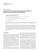
separately evaluated. Figure 1 shows the IEC subgrouping of
bins for 7th and 8th harmonic subgroups and for 7th inter-
harmonic subgroup. The amplitude G
sg,n
(C
isg,n
)ofnth har-
monic (interharmonic) subgroup is defined as the rms value
of all its spectral components, as shown in Figure 1.
Some of the authors of this paper have shown that in the
IEC signal processing framework, a small error in synchro-
nization causes severe spec tral leakage problems and have
proposed advanced signal processing methods that improve
measurement accuracy by reducing sensitivity to desynchro-
nization. The first method makes the IEC grouping compati-
ble with the utilization of Hanning window (HW) instead of
2 EURASIP Journal on Advances in Signal Processing
Voltage sp e ct ru m

time window of 200 ms
Amplitude
340 345 350 355 360 365 370 375 380 385 390 395 400 405 410
Frequency (Hz)
Used for calculating
7th harmonic subgroup
Used for calculating
7th interharmonic subgroup
Used for calculating
8th harmonic subgroup
Figure 1: IEC grouping of “bins” for harmonic and interharmonic subgroups.
RW [3]. Another method, in the framework of synchronized
processing (SP), uses a self-tuning algorithm, synchronizing
the analysed window w idth to an integer multiple of the ac-
tual fundamental period [4]. Finally, a method in the frame-
work of desynchronized processing (DP) is based on a double
stage algorithm: harmonic components are filtered away be-
fore interharmonic evaluation [5–7]. Each of these methods
adopts a technique of smoothing the results over aggregation
intervals g reater than the time window adopted for the anal-
ysis [1, 2]. The increase in complexity of the computational
burden does not always correlate with increased accuracy of
the results.
Other authors of this paper have considered and devel-
oped alternative advanced methods [8–15]. In particular, the
Prony- and ESPRIT-based methods (adaptive Prony method
(APM) and adaptive ESPRIT method (AEM)) appear espe-
cially suitable for solv ing desynchronization (and time vari-
ation) problems warranting a very high level of accuracy.
These methods approximate a sampled waveform as a lin-

ear combination of complex conjugate exponentials and are
not characterized by a fixed frequency resolution. The com-
putational burden of these methods may increase compared
to DFT-based methods when high accuracy is required, but
the increase is still reasonable, especially when using methods
such as AEM.
In this paper, the methods based on the use of the DFT
in the IEC framework are summarized. Then, the methods
based on Prony and ESPRIT theories are reviewed. Finally,
the results of several numerical experiments are reported in
order to compare the different methods in terms of accuracy.
This paper is an extended and improved version of the
paper presented previously at the PES meeting in 2006 [16].
2. DFT-BASED METHODS
In this section, several advanced methods, which use IEC
guidelines and the DFT approach, are reviewed.
2.1. Hanning windowing
The amount of spectral leakage interference depends strictly
on the characteristics of the time window adopted to weight
the signals before the spectral analysis; therefore, an appro-
priate choice can reduce the interference.
The IEC Standard [2] refers to the RW, which is consid-
ered to be the window characterized by the narrowest main
lobe (the best resolution among tones close in frequency),
but with the highest and most slowly decaying side lobes (the
worst interference caused by a strong tone on a weaker tone
not close in frequency). The second type of interaction causes
the greatest problems because of the amplitude difference be-
tween harmonic tones (which may vary in size by hundredths
of a percent up to 100% of the fundamental tone) and inter-

harmonic tones of interest (which are only a few thousandths
of a percent of the size of the fundamental tone).
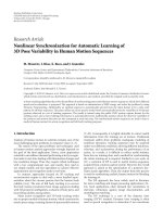
Testa et al. [3] have shown how the Hanning window
can be utilized instead of the rectangular window. In this
case, only minor changes in the IEC procedure are required:
one simply multiplies IEC group values by a factor equal
to (2/3)
1/2
. This reduces the leakage errors on the interhar-
monic groups by about one order of quantity as shown in
Figure 2. It is worth noting that the errors are reported as a
percentage of the amplitude of the close harmonic group and
not of the interested interharmonic group, and are therefore
very relevant.
2.2. Result interpolation
Result interpolation allows one to estimate amplitude, fre-
quency, and phase angle of signal components with great
accuracy, star ting from the results of a DFT performed
at a given frequency resolution (i.e.,
−5 Hz). This method
achieves results similar to those using a higher resolution
analysis.
The interpolation of a given tone is based on the assump-
tion of negligibility of the spectral leakage effects caused by
A. Bracale et al. 3
10
1
0.1
0.01
nth interharmonic

group amplitude error
(nth harmonic (%))
−1 −0.1 −0.01 0.01 0.11
nth harmonic frequency error (Hz)
10
1
0.1
0.01
Rectangular
Hanning
Figure 2: nth interharmonic group amplitude error versus nth har-
monic frequency error: using RW (dotted line) and HW (dashed
line).
the negative frequency replica and the other harmonic and
interharmonic tones. These three conditions occur with a
good approximation if a proper window is used. The authors
selected the Hanning window because of its good spec tral
characteristics and the simplicity of the interpolation formu-
las.
A brief review of the frequency domain interpolation
technique is summarized below.
A sampled and windowed single tone signal is consid-
ered:
s(k)
= A sin

2πf
k
f
S

+ ϕ

·
w(k)withk = 0, 1, , L − 1
(1)
with A being the tone amplitude, f the tone frequency, ϕ
the phase angle, f
S
the sampling frequency, and w a generic
window of length T
W
= L/ f
S
.
Thus, the signal spectrum evaluated by means of the DFT
on L points and neglecting the negative frequency replica
equals
S(i)
=
A · exp( jϕ)
2j
· W

i
L
− ν

with i = 0, 1, , L − 1,
(2)
where ν

= f/f
S
is the tone frequency normalized to the sam-
pling frequency.
In the presence of a small desynchronization between
tone period and sampled time window, none of the DFT
components matches the actual tone frequency as shown in
Figure 3,whereM is the order of the Mth DFT component
and δ is the normalized frequency deviation from the actual
normalized frequency.
Adopting the Hanning window, approximated expres-
sions for the interpolated tone amplitude

A,frequency

f ,and
phase angle
ϕ are

A = π


S(M)



δ

1 −


δ
2

sin(π

δ)
,
ν =
M
L
+

δ,
ϕ =
π
2
+ ∠S(M)
− M · π ·

δ
(3)
Spectral amplitude
1
L
δ
M
− 3
L
M
− 1

L
M
L
ν
M +1
L
Normalized frequency
Spectrum
DFT
Figure 3: Example of the spectrum (dashed line) and DFT compo-
nents (
•)ofasignal.
being
|

δ|=
2 − α
1+α
, α
=


S(M)




S

M +sign(


δ)



(4)
with sign(

δ) = sign(|S(M +1)|−|S(M − 1)|).
2.3. Desynchronized processing
In the following section, the method proposed in [ 6]—
that constitutes an example of desynchronized processing—
is briefly recalled. It is based on harmonic filtering before the
interharmonic analysis.
Harmonic filtering
A sampled and windowed time domain signal is considered:
s
w

(k) = s(k) · w

(k)withk = 0, 1, , L − 1, (5)
where s is the signal and w

the adopted window. It can be
represented by the sum of two contributes, one harmonic
and the other interharmonic:
s
w


(k) =

s
H
(k)+s
I
(k)

· w

(k)withk = 0, 1, , L − 1.
(6)
The evaluation of the amplitude

A
H
n
, of the normalized
frequency
ν
n
, and of the phase ϕ
n
, of each harmonic compo-
nent gives
s
H
(k) =

n


A
H
n
sin

2πν
n
k + ϕ
n

with k = 0, 1, , L − 1.
(7)
This contribution can be filtered from the original signal,
for instance, in the time domain:
s
I
(k) = s(k) − s
H
(k)withk = 0, 1, , L − 1. (8)
The only w ay to eliminate spectral leakage effects is to
have a very accurate estimation of the frequency, amplitude,
4 EURASIP Journal on Advances in Signal Processing
and phase angle of the harmonic components to be filtered.
This can be a ccomplished by proper inter polation of the
spectrum samples calculated by DFT [6, 7], such as that il-
lustrated in Section 2.2.
Interharmonic analysis
Once
s

I
(k) has been obtained, an interharmonic analysis can
be performed with reduced harmonic leakage effects. The
surviving harmonic leakage is given by
ε
H
(k) = s
H
(k) − s
H
(k)withk = 0, 1, , L − 1. (9)
This is generally different from zero. The lower ε
H
is equal to
the lower leakage effects.
The use of a proper window w

for the interharmonic
analysis can reduce the residual harmonic leakage problems:
s
I
w

(k) = s
I
(k) · w

(k)withk = 0, 1, , L − 1. (10)
Thechoiceofw


must be made by considering addi-
tional aspects [3], such as interharmonic tone interaction
and IEC grouping problems. Here, reference is made only to
the HW.
Accuracy and computational burden
The accuracy is related to the filtering accuracy, which de-
pends on the interpolation algorithms, the number of sam-
ples analysed, and interferences, such as those produced by
interharmonic tones close to the harmonics (which need to
be estimated and filtered).
With regard to the computational burden, it is important
to note that to achieve accuracy of equal or greater level than
that of synchronized methods, an exact synchronization is
not needed. It is therefore possible to choose a sampling fre-
quency f

S
, independent from the actual supply frequency,
but still referring to its rated value. This allows one to acquire
a number of samples using the power of two:
f

S
=
2
n
10T
1r
=
f

1r
2
n
10
(11)
with T
1r
and f
1r
being the rated values of the system’s funda-
mental period and frequency, respectively.
The technique generally implies a doubled number of
FFT. It is worth noting that by using the same window for
both the first and second stages, harmonic components can
be directly filtered in the frequency domain due to the DFT
linearity [6].
2.4. Smoothing of the results
In the IEC standards [1, 2], it is highly recommended to pro-
vide a smoothing of the results obtained during the analyses.
Smoothed results are derived from the components obtained
in 200 milliseconds analyses as an average over 15 contiguous
time windows, updated either every time window (approx-
imately every 200 milliseconds) or every 15 time windows
(about 3 s each). This procedure may affect the accuracy of
the results when the desynchronization effects are remark-
able in the 200- milliseconds window.
3. PRONY- AND ESPRIT-BASED METHODS
In this section, Prony and ESPRIT methods are briefly re-
called, and then advanced versions of these methods (adap-
tive Prony and ESPRIT methods) based on the use of proper

time windows are analysed [8–16].
3.1. The Prony method
Let the signal sampled data [
x(1) x(2)
··· x(N)
]beap-
proximated with the following linear combination of M
complex exponentials
1
[17]:
x(n) =
M

k=1
h
k
z
(n−1)
k
n = 1, 2, , N, (12)
where h
k
= A
k
e
jψ
k
, z
k
= e

(α
k
+ jω
k
)T
s
, k is the exponential code,
T
s
is the sampling time, A
k
is the amplitude, ψ
k
is the ini-
tial phase, ω
k
= 2πf
k
is the angular velocity, and α
k
is the
damping factor.
The problem is to find damping factors, initial phases,
frequencies, and amplitudes solving the following nonlinear
problem:
min
N

n=1




x(n) − x(n)


2
. (13)
The Prony idea consists of first solving the following set
of linear equations to find the damping factors and frequen-
cies [17]:
M

m=0
a(m)x( n − m) = 0, (14)
where n
= M +1,M +2, , N. The (N − M) relations (14)
constitute a linear equation system in M unknowns (i.e., the
a(m)coefficients).
If N
= 2M, the system (14) can be solved in closed
form since it represents an M-equation system with the same
number of unknowns. In practice, the available samples are
N>2M, so an estimation problem has to be solved since the
number of (14) are greater than the number of unknowns M
(N
− M>M). In this case, the M unknown coefficients a(m)
can be obtained by minimizing the total error:
E
T
=

N

n=M+1
M

m=0
a(m)x( n − m). (15)
Once known the a(m)coefficients, the damping factors
and the frequencies of each exponential are calculated by
means of simple relations.
The amplitudes and phases of each exponential are then
calculated by solving a second set of linear equations linking
these unknowns to the sampled data.
1
It has been shown that the best choice of the number M of complex ex-
ponentials for power system applications relies on using the minimum
description length method [10].
A. Bracale et al. 5
3.2. The ESPRIT method
The original ESPRIT algorithm [17–19]isbasedonnatu-
rally existing shift invariance between the discrete time series,
which leads to rotational invariance between the correspond-
ing signal subspaces.
The assumed signal model is the following:
x(n) =
M

k=1
A
k

e
( jω
k
n)
k
+ w(n), (16)
where w(n) represents additive noise. The eigenvectors U of
the autocorrelation matrix

R
x
of the signal define two sub-
spaces S
1
and S
2
(signal and noise subspaces) by using two
selector matrices Γ
1
and Γ
2
:
S
1
= Γ
1
U, S
2
= Γ
2

U. (17)
The rotational invariance between both subspaces leads
to the equation
S
1
= ΦS
2
, (18)
where
Φ
=
⎡
⎢
⎢
⎢
⎢
⎣
e
jω
1
0 ··· 0
0 e
jω
2
··· 0
.
.
.
.
.

.
.
.
.
.
.
.
00
··· e
jω
M
⎤
⎥
⎥
⎥
⎥
⎦
. (19)
The matrix Φ contains all information about M compo-
nents’ frequencies. Additionally, the TLS (total least-squares)
approachassumesthatbothestimatedmatricesS
1
and S
2
can
contain er rors and find the matrix Φ by means of minimiza-
tion of the Frobenius norm of the error matrix. Amplitudes
of the components can be found by properly using the auto-
correlation matrix


R
x
of the signal; alternatively, a mplitudes
and phases (introduced in the signal model) can be found in
similar way as with the Prony method by solving a second set
of linear equations [20].
3.3. The adaptive Prony and adaptive ESPRIT methods
The basic idea of these methods consists in applying the
PronyorESPRITmethodstoanumberof“short contigu-
ous time windows” inside the sig nal [11]; the widths of these
short time windows are variable, and this variability ensures
the best fitting of the waveform time variations.
To select the most adequate short contiguous time win-
dows, let us initially refer to the adaptive Prony method
(APM) and consider the signal x(t) in a time observation
period T
obs
with L samples obtained using the sampling fre-
quency f
S
= 1/T
s
. The following mean square relative error
can be considered:
ε
2
curr
=
1
L

L

k=1


x

t
k

− x

t
k



2
x

t
k

2
, (20)
where t
k
= kT
s
(k = 1, 2, 3, , L)andx(t

k
)isgivenby(12).
The mean square relative error ε
2
curr
gives a measure of the fi-
delity of the model considered; in fact, it represents the mean
square relative error of the model estimation.
By defining a threshold ε
2
thr
(acceptable mean square rel-
ative error), it is possible to choose in the time observation
period a short time window [t
i
, t
f
] (or for fixed sampling fre-
quency, a subset of the data segment length can be used) en-
suring the satisfactory approximation (ε
2
curr
≤ ε
2
thr
).
The main steps of the APM algorithm are the following:
(i) select a starting short time window width T
min
;

(ii) apply the Prony method to the samples in the short
time window to obtain the model parameters (ampli-
tudes, damping factors, frequencies, and initial phases
of the Prony exponentials);
(iii) use the exponentials obtained in step (ii) to calculate
ε
2
curr
with (20);
(iv) compare ε
2
curr
with the threshold ε
2
thr
and
(a) if ε
2
curr
≤ ε
2
thr
, store the Prony model exponential
parameters and increase the short time window
width (and then the subset of the data segment)
until ε
2
curr
≤ ε
2

thr
and t
f
≤ T
obs
, and then go to
step (v);
(b) if ε
2
curr
is greater than the threshold ε
2
thr
, increase
the short time window width and go to step (vi);
(v) store the short time spectral components and select a
new starting short time window width;
(vi) compare t
f
with T
obs
;ift
f
is less than or equal to the
observation period, go to step (ii); if t
f
is greater than
T
obs
, first calculate and store short time spectral compo-

nents and then stop.
It should be noted that in step (iv)(a), the short time win-
dow w idth is increased until the condition ε
2
curr
≤ ε
2
thr
is sat-
isfied; the Prony model parameters remain fixed at the values
that satisfy the criterion the first time. In this way, a nonneg-
ligible reduction of the computational efforts arises, mainly
in the presence of slight time-varying waveforms.
The APM is generally characterized by very good accu-
racy in the assessment of waveform distortion in power sys-
tems, but its computational burden is certainly greater than
the DFT methods; the computational efforts may be worth-
while when increased accuracy is required.
Let us consider now the case of the adaptive ESPRIT
method (AEM). As for APM, we apply the ESPRIT method
to a number of “short contiguous time windows.”
The main steps of the AEM algorithm include the follow-
ing:
(i) select a starting short time window width T
min
;
(ii) estimate the autocorrelation matrix

R
x

of the signal us-
ing the samples in the short time window;
(iii) calculate the eigenvalues of

R
x
and then, matrices S
1
and S
2
;
(iv) estimate the matrix Φ;
(v) calculate the eingenvalues of the matrix Φ and then,
the frequencies of the exponentials;
6 EURASIP Journal on Advances in Signal Processing
(vi) calculate the amplitudes and arguments of the expo-
nentials in a similar way to the Prony method, for as-
signed frequencies (step (v)) and damping factors
2
;
(vii) use the exponential parameters obtained to calculate
ε
2
curr
with (20);
(viii) compare ε
2
curr
with the threshold ε
2

thr
and
(a) if ε
2
curr
≤ ε
2
thr
, store the exponential parameters
and increase the short time window width (and
then the subset of the data segment) until ε
2
curr
≤
ε
2
thr
and t
f
≤ T
obs
, and then go to s tep (ix);
(b) if ε
2
curr
is greater than the threshold ε
2
thr
, increase
the short time window width and go to step (x);

(ix) store the short time spectral components and select a
new starting short time window width;
(x) compare t
f
with T
obs
.Ift
f
is less than or equal to the
observation period T
obs
, go to step (ii). If t
f
is greater
than T
obs
, first calculate and store short t ime spectral
components, and then go to stop.
3.4. Considerations
The Prony- and ESPRIT-based methods have the following
features:
(i) the window width is free and only linked to the signal
waveform characteristics;
(ii) the adaptive version ensures the best fit of waveform
variations by an optimal choice of the time window
width;
(iii) window width does not constrain the frequency reso-
lution.
The AEM is also characterized by excellent accuracy in
the assessment of waveform distortion in power systems; its

computational burden is greater than the DFT methods, but
generally sig nificantly lower than that required by APM.
In practice, a comprehensive analytical comparison of
AEM and APM computational efforts cannot be stated with
general validity, since AEM and APM use different models to
approximate the waveforms. Because of this, AEM and APM
can be characterized not only by a different number of short
contiguous time windows in the time observation period T
obs
but also each short contiguous time window may have a differ-
ent number M of complex exponentials used to approximate
the waveform.
However, some considerations can help demonstrate the
reduced computational effort of AEM. These reduced com-
putational efforts have been tested using several numerical
applications performed on simulated and measured station-
ary/nonstationary waveforms, like the examples reported in
Section 4.
First, the AEM method generally requires fewer short con-
tiguous time windows in the time observation period T
obs
2
Since in distortion assessment in power systems, the waveforms can be
considered to be the sum of sinusoids, the damping factors value can be
constrained to zero.
than APM. This is due to the fact that to b etter estimate
the matrix

R
x

a sig nificant number of samples are necessary.
Therefore, enlarging the dimension of the short contiguous
time windows and reducing the number of short contiguous
time w indows in the time observation period T
obs
are often
requirements for AEM.
Moreover, since the APM model does not include the
presence of noise, it generally requires a larger number M of
complex exponentials to approximate the waveform in each
of the short contiguous time windows.
Finally, it should be noted that, the DFT-based methods
are generally faster than the parametric methods, so that on
the basis of our experience the rank of computational burden
of the methods, from faster to slower, is
(1) DFT-based methods;
(2) adaptive ESPRIT method;
(3) adaptive Prony method.
4. NUMERICAL EXPERIMENTS
Several numerical experiments were performed. In consider-
ation of space, reference is made only to the results of four
case studies.
The examples were performed by utilizing the IEC nor-
mal approach (IEC-N) characterised by RW and T
W
=
200 milliseconds [1, 2], the interpolation technique (I-HW)
described in Section 2.2 applied to the components obtained
by DFT on 200 milliseconds using HW, the desynchronised
procedure (IEC-DP) described in Section 2.3 , and the adap-

tive Prony (APM) and adaptive ESPRIT methods (AEM) de-
scribed in Section 3.3.
All the data used in the experimental case studies were
entered with the maximum allowable precision. The exact
number of zeroes after the last significant cipher is not re-
ported for the sake of simplicity. The results obtained are al-
ways reported in diagrams using two figures for DFT-based
and high-resolution methods (APM and AEM). Two differ-
ent scales for errors are used for high-resolution methods:
left- side scale for APM and right-side scale for AEM.
The sampling frequency for all the experiments and all
the methods used is 5 kHz. The window width used is always
T
w
= 200 milliseconds for DFT-based methods. The win-
dow width varies from a minimum of 20 milliseconds (case-
studies 1–3) to a maximum of 220 milliseconds (case study
4) for APM and AEM, but all results are presented with ref-
erence to 200 milliseconds [11], for ease of comparison of the
methods.
It should be noted that the number of samples can af-
fect only the computational burden of DFT-based methods,
in fact the FFT algorithm is faster when a number of s am-
ples that is a power of two is chosen. With reference to APM
and AEM methods, the adaptive algorithm selects a variable
number of samples (for each short contiguous time window)
to fit at best the waveform considered; this number does not
affect these methods.
The acceptable mean square relative error for APM and
AEM is ε

= 1.0 · 10
−15
.
A. Bracale et al. 7
0.5
0
−0.5
−1
−1.5
−2
−2.5
−3
C
isg,1
magnitude error (%)
70 71 72 73 74 75 76 77 78 79 80
Interharmonic frequency (Hz)
< 3.5
× 10
−3
IEC-DP
IEC-N
(a)
×10
−6
1.5
1
0.5
0
−0.5

−1
−1.5
APM C
isg,1
magnitude error (%)
70 71 72 73 74 75 76 77 78 79 80
Interharmonic frequency (Hz)
×10
−9
4
2
0
−2
−4
−6
−8
−10
AEM C
isg,1
magnitude error (%)
APM
AEM
(b)
Figure 4: Case study 1: interharmonic subgroup C
isg,1
magnitude error (in %) versus interharmonic frequency: (a) IEC-N (-·-Δ)andIEC-
DP (dotted line
◦), (b) APM (dotted line +) and AEM (dotted line ).
4.1. Case study 1
The signal considered is constituted by a tone of a mplitude

1 pu at the fundamental frequency of 50 Hz with an inter-
harmonic tone of amplitude 0.001 pu at varying frequencies
(ranging from 70 Hz to 80 Hz in increments of 1 Hz). Figures
4(a) and 4(b) report the results in terms of magnitude error
for the interharmonic subgroup C
isg,1
versus the frequency of
the interharmonic component in the eleven experiments.
The errors of IEC-N reach the value of about
−3% un-
der the worst conditions, 73 Hz and 78 Hz; the error is null
in the experiments characterised by interharmonic frequen-
cies of 70 Hz, 75 Hz, and 80 Hz, where the interharmonic is
synchronised with T
w
.
TheerrorsofIEC-DParenotperceptiblesincetheyreach
the value of about 3.5
× 10
−3
%. The errors of APM do not
reach 1.5
× 10
−6
%, while the errors of AEM do not reach
1.0
× 10
−8
%.
In Figure 5, results obtained by I-HW (Figure 5(a)), and

AEP-AEM (Figure 5(b)) are compared. In particular, in-
terharmonic component amplitude, phase angle, and fre-
quency percentage error versus interharmonic frequency are
reported. All methods perform very well.
Figure 6 reports the interharmonic component per-
centage error versus interharmonic frequency, smoothing
the results over 15 intervals of 200 milliseconds for I-HW
(Figure 6(a)) and APM and AEM (Figure 6(b)). Only the
amplitude and frequency estimations are reported because
smoothing the phase angle results does not make sense.
Again, all methods perform very well, w ith the most bene-
fits gained using the I-HW method.
4.2. Case study 2
The case study parameters are the same as in case study
1, except the fundamental tone frequency was changed to
50.02 Hz in order to introduce a further kind of desynchro-
nization
3
; in fact, the window width adopted for the DFT
based methods remains equal to 200 milliseconds.
Figures 7 and 8 are the equivalent of Figures 4 and 5.
Comparing Figures 4 and 7, it is possible to observe that
while APM and AEM maintain similar performances, the er-
rors of IEC-N reach dramatic values over 200% due to the
spectral leakage of RW; IEC-DP, which has been introduced
for these kinds of problems, contains errors to a maximum
value of 3.5
× 10
−3
%. Comparing Figures 5 and 8, it is possi-

ble to observe that the performances remain very good with
a slight reduction in the accuracy for APM; the behaviour of
AEM is very good.
Figure 9 reports the fundamental component percentage
error versus interharmonic frequency for I-HW (Figure 9(a))
and APM-AEM (Figure 9(b)) in terms of amplitude, phase
angle, and frequency. All methods give very good results.
Note the results of the Prony- and ESPRIT-based methods
with regard to the amplitude and the results of all the meth-
ods with regard to frequency. Excellent performances are
guaranteed by using AEM, which is characterized by errors
that are always lower than 10
−11
%.
4.3. Case study 3
The signal considered is constituted by a tone of amplitude
1 pu at a fundamental frequency of 50 Hz and by a couple of
interharmonic tones of amplitude 0.001 pu, located at sym-
metrical frequency positions starting from 75 Hz; the first
starts at 70 Hz and varies its frequency to 75 Hz by incre-
ments of 1 Hz, while the second starts at 80 Hz and varies its
frequency to 75 Hz by decrements of 1 Hz. Six experiments
were performed.
3
Such desynchronization results are comparable with the accuracy of IEC
instruments of Class A.
8 EURASIP Journal on Advances in Signal Processing
×10
−4
2

0
−2
−4
I-HW magnitude
error (%)
70 71 72 73 74 75 76 77 78 79 80
×10
−3
1.5
1
0.5
0
I-HW phase
error (%)
70 71 72 73 74 75 76 77 78 79 80
×10
−4
2
0
−2
I-HW frequency
error (%)
70 71 72 73 74 75 76 77 78 79 80
Interharmonic frequency (Hz)
I-HW
(a)
×10
−6
5
0

−5
−10
APM magnitude
error (%)
70 71 72 73 74 75 76 77 78 79 80
×10
−8
1
0.5
0
−0.5
−1
AEM magnitude
error (%)
×10
−7
2
1
0
−1
APM phase
error (%)
70 71 72 73 74 75 76 77 78 79 80
×10
−10
1
0.5
0
−0.5
AEM phase

error (%)
×10
−9
4
2
0
−2
APM frequency
error (%)
70 71 72 73 74 75 76 77 78 79 80
×10
−10
2
0
−2
AEM frequency
error (%)
Interharmonic frequency (Hz)
APM
AEM
(b)
Figure 5: Case study 1: interharmonic amplitude, phase angle, and frequency error (in %) versus interharmonic frequency: (a) I-HW (dotted
line x), (b) APM (dotted line +) and AEM (dotted line ).
×10
−9
20
15
10
5
0

−5
I-HW magnitude
error (%)
70 71 72 73 74 75 76 77 78 79 80
×10
−10
2
1.5
1
0.5
0
−0.5
−1
I-HW frequency
error (%)
70 71 72 73 74 75 76 77 78 79 80
Interharmonic frequency (Hz)
I-HW
(a)
×10
−7
8
6
4
2
0
−2
−4
APM magnitude
error (%)

70 71 72 73 74 75 76 77 78 79 80
×10
−9
3
2
1
0
−1
−2
−3
AEM magnitude
error (%)
×10
−9
3
2
1
0
−1
APM frequency
error (%)
70 71 72 73 74 75 76 77 78 79 80
×10
−10
1.5
1
0.5
0
−0.5
−1

−1.5
AEM frequency
error (%)
Interharmonic frequency (Hz)
APM
AEM
(b)
Figure 6: Case study 1: interharmonic amplitude and frequency error (in %) versus interharmonic frequency by smoothing the results over
15 intervals of 200 milliseconds: (a) I-HW (dotted line x), (b) APM (dotted line +) and AEM (dotted line ).
Figure 10 reports the results in terms of magnitude er-
ror for the interharmonic subgroup C
isg,1
versus the abso-
lute value of the distance of each interharmonic component
from 75 Hz in the six experiments. In this case, IEC-based
methods (Figure 10(a))suffer significantly from the interfer-
ence problems between the two interharmonics caused by
their proximity to one another. IEC-DP behaves the worst
because of the larger main lobes derived from the use of
the Hanning window. Both IEC-N and IEC-DP show null
error when the two components are superimposed on each
A. Bracale et al. 9
250
200
150
100
50
0
−50
C

isg,1
magnitude error (%)
70 71 72 73 74 75 76 77 78 79 80
Interharmonic frequency (Hz)
< 3.5
× 10
−3
IEC-N
IEC-DP
(a)
×10
−6
8
6
4
2
0
−2
−4
−6
APM C
isg,1
magnitude error (%)
70 71 72 73 74 75 76 77 78 79 80
Interharmonic frequency (Hz)
×10
−9
6
4
2

0
−2
−4
−6
−8
−10
AEM C
isg,1
magnitude error (%)
APM
AEM
(b)
Figure 7: Case study 2: interharmonic subgroup C
isg,1
magnitude error (in %) versus interharmonic frequency: (a) IEC-N (-·-Δ)andIEC-
DP (dotted line
◦), (b) APM (dotted line +) and AEM (dotted line ).
×10
−3
10
5
0
−5
I-HW magnitude
error (%)
70 71 72 73 74 75 76 77 78 79 80
×10
−3
5
0

−5
−10
I-HW phase
error (%)
70 71 72 73 74 75 76 77 78 79 80
×10
−3
2
1
0
−1
I-HW frequency
error (%)
70 71 72 73 74 75 76 77 78 79 80
Interharmonic frequency (Hz)
I-HW
(a)
×10
−5
4
2
0
−2
APM magnitude
error (%)
70 71 72 73 74 75 76 77 78 79 80
×10
−8
1
0

−1
AEM magnitude
error (%)
×10
−7
5
0
−5
APM phase
error (%)
70 71 72 73 74 75 76 77 78 79 80
×10
−10
2
1
0
−1
AEM phase
error (%)
×10
−8
1
0
−1
APM frequency
error (%)
70 71 72 73 74 75 76 77 78 79 80
×10
−10
1

0
−1
−2
AEM frequency
error (%)
Interharmonic frequency (Hz)
APM
AEM
(b)
Figure 8: Case study 2: interharmonic amplitude, phase angle, and frequency error (in %) versus interharmonic frequency: (a) I-HW (dotted
line x), (b) APM (dotted line +) and AEM (dotted line ).
other at 75 Hz and synchronized w ith T
w
=200 milliseconds.
APM and AEM (Figure 10(b)) still give good results, but not
as good as in the previous case studies.
Figure 11 reports the interharmonic subgroup C
isg,1
mag-
nitude error (in %) versus the distance of interharmonic
tones from 75 Hz obtained by smoothing the results of 15
intervals of 200 milliseconds for IEC-N, IEC-DP (Figure
11(a)), and APM and AEM (Figure 11(b)). IEC-based meth-
ods exhibit improved performances; in particular, IEC-DP
drastically reduces the errors, except for the distance of 5 Hz,
which is the synchronized condition in which no effects are
gained from smoothing.
10 EURASIP Journal on Advances in Signal Processing
×10
−2

−11
−10
I-HW magnitude
error (%)
70 71 72 73 74 75 76 77 78 79 80
×10
−4
5
0
−5
I-HW phase
error (%)
70 71 72 73 74 75 76 77 78 79 80
×10
−4
2
0
−2
I-HW frequency
error (%)
70 71 72 73 74 75 76 77 78 79 80
Interharmonic frequency (Hz)
I-HW
(a)
×10
−8
2
0
−2
APM magnitude

error (%)
70 71 72 73 74 75 76 77 78 79 80
×10
−11
2
0
−2
−4
AEM magnitude
error (%)
×10
−10
5
0
−5
APM phase
error (%)
70 71 72 73 74 75 76 77 78 79 80
×10
−14
5
0
−5
AEM phase
error (%)
×10
−8
2
0
−2

APM frequency
error (%)
70 71 72 73 74 75 76 77 78 79 80
×10
−13
1
0
−1
AEM frequency
error (%)
Interharmonic frequency (Hz)
APM
AEM
(b)
Figure 9: Case study 2: fundamental component amplitude, phase angle, and frequency error (in %) versus interharmonic frequency: (a)
I-HW (dotted line x), (b) APM (dotted line +) and AEM (dotted line ).
20
10
0
−10
−20
−30
−40
C
isg,1
magnitude error (%)
01 23 45
Interharmonic frequency distance (Hz)
IEC-N
IEC-DP

(a)
×10
−3
2
1.5
1
0.5
0
−0.5
−1
−1.5
APM C
isg,1
magnitude error (%)
012345
Interharmonic frequency distance (Hz)
×10
−7
0.5
0
−0.5
−1
−1.5
−2
−2.5
−3
−3.5
AEM C
isg,1
magnitude error (%)

APM
AEM
(b)
Figure 10: Case study 3: interharmonic subgroup C
isg,1
magnitude error (in %) versus the distance of interharmonic tones from 75 Hz: (a)
IEC-N (-
·-Δ) and IEC-DP (dotted line ◦), (b) APM (dotted line +) and AEM (dotted line ).
4.4. Case study 4
The signal considered is constituted by a 1 pu fifth harmonic
tone at a frequency which varies from 249 Hz to 251 Hz by in-
crements of 0.5 Hz, giving five different base conditions. Two
interharmonic tones of amplitudes 0.1 pu are also present;
their frequency position is centred on the fifth harmonic fre-
quency and their frequency interdistance is 8, 10, and 12 Hz,
giving three cases for each base condition. Therefore, this sit-
uation represents a fifth harmonic tone carrier which suffers
from a maximum fundamental frequency desynchronization
of 0.2 Hz and whose amplitude is modulated at 4, 5, and
6 Hz, with a modulation amplitude of 0.2 pu.
Figure 12 reports the harmonic subgroup G
sg,5
magni-
tude error (in %) versus the carrier frequency for the three
modulation frequencies when using IEC-DP (Figure 12(a)),
A. Bracale et al. 11
10
8
6
4

2
0
−2
−4
C
isg,1
magnitude error (%)
01 23 45
Interharmonic frequency distance (Hz)
< 3.5
× 10
−3
IEC-N
IEC-DP
(a)
×10
−4
4
2
0
−2
−4
−6
−8
−10
−12
APM C
isg,1
magnitude error (%)
012345

Interharmonic frequency distance (Hz)
×10
−8
2
1
0
−1
−2
−3
−4
−5
−6
−7
−8
AEM C
isg,1
magnitude error (%)
APM
AEM
(b)
Figure 11: Case study 3: interharmonic subgroup C
isg,1
magnitude error (in %) versus the distance of interharmonic tones from 75 Hz with
smoothed results over 15 intervals of 200 milliseconds: (a) IEC-N (-
·-Δ) and IEC-DP (dotted line ◦), (b) APM (dotted line +) and AEM
(dotted line ).
APM (Figure 12(b)), and AEM (Figure 12(c)). IEC-DP suf-
fers from the presence of low frequency modulations, behav-
ing acceptably for a modulating frequency of 5 Hz; Prony and
ESPRIT methods show similar levels of accuracy for the three

modulation frequencies.
Figure 13 shows harmonic subgroup G
sg,5
magnitude er-
ror (in %) versus interharmonic frequency, smoothing the
results of 15 intervals of 200 milliseconds for the IEC-DP
method. The benefits derived from smoothing are evident.
The smoothing of APM and AEM results does not change
the accuracy of these methods and is therefore not reported.
Figure 14 reports the interharmonic subgroup C
isg,5
mag-
nitude versus the carrier frequency for the three modulation
frequencies for IEC-DP (Figure 14(a)), APM (Figure 14(b));
the results for AEM are not reported because they are all
equal to zero, that is the true magnitude of this subgroup.
IEC-DP captures the spectral leakage of the fifth harmonic
and of the interharmonics that are in the adjacent harmonic
subgroup, giving misleading results; on the contrary, results
obtained using the Prony and ESPRIT methods confirm their
insensitivity to this phenomenon.
5. CONCLUSIONS
One of the main problems for waveform distortion assess-
ment has been considered which examines how to reduce
the effects of spectral leakage due to fundamental frequency
desychronization and harmonics on interharmonic compo-
nents.
The signal processing aspects of the problem have been
considered; different proposals regarding both DFT-based
and advanced methods (Prony and ESPRIT) have been re-

called and compared to each other. The results of several nu-
merical experiments have been reported and analysed.
The main outcomes of the paper are the following:
(i) IEC standards, even if characterized by simplicity,
may suffer dramatic inaccuracy problems under con-
ditions such as those characterized by f undamental
and harmonic desynchronization within the time win-
dow widths;
(ii) DFT advanced methods can remarkably reduce the
inaccuracies caused by the spectral leakage with-
out remarkably increasing computational burden, and
therefore could be utilized in industrial applications;
(iii) in particular circumstances, which stress the behaviour
of the DFT methods, DFT advanced methods (even
if combined w ith smoothing) may give inaccuracies
with very high values for interharmonic subgroups
and components;
(iv) adaptive Prony and ESPRIT methods do not seem to
suffer at all from the spectral leakage phenomenon
even in very critical conditions;
(v) the computational burden of APM and AEM is greater
when compared to DFT-based methods when high ac-
curacy is required, but this burden is reasonable with
respect to the accuracy of the results obtained, espe-
cially when using AEM;
(vi) the reliability of the adaptive Prony and ESPRIT meth-
ods in addition to their unlimited frequency resolution
suggest that they should be utilized as reference meth-
ods for research purposes, especially when computa-
tion burden is not a concern.

12 EURASIP Journal on Advances in Signal Processing
8
6
4
2
0
−2
−4
−6
−8
IEC-DP G
isg,5
magnitude error (%)
249 249.5 250 250.5 251
Carrier frequency (Hz)
Modulation frequency 4 Hz
Modulation frequency 5 Hz
Modulation frequency 6 Hz
(a)
×10
−6
3
2
1
0
−1
−2
−3
−4
−5

APM G
isg,5
magnitude error (%)
249 249.5 250 250.5 251
Carrier frequency (Hz)
Modulation frequency 4 Hz
Modulation frequency 5 Hz
Modulation frequency 6 Hz
(b)
×10
−11
4
3
2
1
0
−1
−2
−3
−4
−5
AEM G
isg,5
magnitude error (%)
249 249.5 250 250.5 251
Carrier frequency (Hz)
Modulation frequency 4 Hz
Modulation frequency 5 Hz
Modulation frequency 6 Hz
(c)

Figure 12: Case study 4: harmonic subgroup G
sg,5
magnitude error
(in %) versus the carrier frequency for three modulation frequen-
cies: (a) IEC-DP (dotted line
◦), (b) APM (dotted line +) and (c)
AEM (dotted line ).
8
6
4
2
0
−2
−4
−6
−8
IEC-DP G
isg,5
magnitude error (%)
249 249.5 250 250.5 251
Carrier frequency (Hz)
Modulation frequency 4 Hz
Modulation frequency
5Hz
Modulation frequency
6Hz
Figure 13: Case study 4: harmonic subgroup G
sg,5
magnitude error
(in %) versus interharmonic frequency, smoothing the results over

15 intervals of 200 milliseconds for the IEC-DP (dotted line
◦).
0.15
0.1
0.05
0
−0.05
−0.1
IEC-DP C
isg,5
magnitude
249 249.5 250 250.5 251
Carrier frequency (Hz)
Modulation frequency 4 Hz
Modulation frequency 5 Hz
Modulation frequency 6 Hz
(a)
×10
−14
4.5
4
3.5
3
2.5
2
1.5
1
0.5
0
APM C

isg,5
magnitude
249 249.5 250 250.5 251
Carrier frequency (Hz)
Modulation
frequency 4 Hz
Modulation
frequency 5 Hz
Modulation
frequency 6 Hz
(b)
Figure 14: Case study 4: interharmonic subgroup C
isg,5
magnitude
versus the carrier frequency for three modulation frequencies: (a)
IEC-DP (dotted line
◦), (b) APM (dotted line +).
A. Bracale et al. 13
ACKNOWLEDGMENT
This work was partly supported by the Italian Ministry for
University and Research.
REFERENCES
[1] IEC standard 61000-4-30, “Testing and measurement techni-
ques—Power quality measurement methods,” Ed. 2003.
[2] IEC standard 61000-4-7, “General guide on harmonics and
interharmonics measurements, for power supply systems and
equipment connected thereto,” Ed. 2002.
[3] A. Testa, D. Gallo, and R. Langella, “On the processing of har-
monics and interharmonics: using hanning window in stan-
dard framework,” IEEE Transactions on Power Delivery, vol. 19,

no. 1, pp. 28–34, 2004.
[4] D. Gallo, R. Langella, and A. Testa, “A self-tuning harmonic
and interharmonic processing technique,” European Transac-
tions on Electrical Power, vol. 12, no. 1, pp. 25–31, 2002.
[5] D. Gallo, R. Langella, and A. Testa, “Interharmonic analysis
utilising optimised harmonic filtering,” in Proceedings of IEEE
International Symposium on Diagnostic or Electrical Machines,
Power Electronics and Drives (SDEMPED ’01), Gorizia, Italy,
September 2001.
[6] D. Gallo, R. Langel la, and A. Testa, “Desynchronized process-
ing technique for harmonic and interharmonic analysis,” IEEE
Transactions on Power Delivery, vol. 19, no. 3, pp. 993–1001,
2004.
[7] P. Langlois and R. Bergeron, “Interharmonic analysis by a fre-
quency interpolation method,” in Proceedings of the 2nd Inter-
national Conference on Power Quality (PQA ’92), Atlanta, Ga,
USA, September 1992.
[8] A. Bracale, G. Carpinelli, D. Lauria, Z. Leonowicz, T. Lobos,
and J. Rezmer, “On some spectrum estimation methods for
analysis of non-stationary signals in power systems—part I:
theoretical aspects,” in Proceedings of the 11th International
Conference on Harmonics and Quality of Power (ICHQP ’04),
pp. 266–271, Lake Placid, NY, USA, September 2004.
[9] A. Bracale, G. Carpinelli, Z. Leonowicz, T. Lobos, and J.
Rezmer, “Spectrum estimation of non-stationary signals in
traction systems,” in Proceedings of the International Confer-
ence on Power Systems (ICPS ’04), pp. 821–826, Kathmandu,
Nepal, November 2004.
[10] A. Bracale, P. Caramia, and G. Carpinelli, “Optimal evalua-
tion of waveform distortion indices with Prony and rootmusic

methods,” to appear in International Journal of Power and En-
ergy Systems.
[11] A. Bracale, P. Caramia, and G. Carpinelli, “Adaptive Prony
Method for Waveform Distortion Detection in Power Sys-
tems,” to appear in International Journal on Electrical Power
and Energy Systems.
[12] Z. Leonowicz, T. Lobos, and J. Rezmer, “Advanced spectrum
estimation methods for signal analysis in power electronics,”
IEEE Transactions on Industrial Electronics, vol. 50, no. 3, pp.
514–519, 2003.
[13] A. Br acale, D. Proto, and P. Varilone, “Adaptive Prony method
for spectrum estimation of non-stationary signals in trac-
tion systems,” in Proceedings of the International Conference on
Computer as a Tool (EUROCON ’05), vol. 2, pp. 1550–1553,
Belgrade, Serbia & Montenegro, November 2005.
[14] A. Bracale, G. Carpinelli, and L. Piegari, “Adaptive Prony
method for an accurate analysis of AC waveform distortions
caused by adjustable speed drives,” in Proceedings of the 12th
International Conference on Harmonics and Quality of Power
(ICHQP ’06), Cascais, Portugal, October 2006.
[15] A. Bracale, G. Carpinelli, Z. Leonowicz, T. Lobos, and J.
Rezmer, “Measurement of IEC groups and subgroups using
advanced spectrum estimation methods,” in Proceedings of the
23rd IEEE Instrumentation and Measurement Technology Con-
ference (IMTC ’06), pp. 1015–1020, Sorrento, Italy, April 2006.
[16] A. Bracale, G. Carpinelli, R. Langella, and A. Testa, “On some
advanced methods for waveform distortion assessment in
presence of interharmonics,” in Proceedings of IEEE Power En-
gineering Society General Meeting,p.8,Monreal,QC,Canada,
June 2006.

[17] S. M. Kay, Modern Spectral Estimation: Theory and Application,
Prentice-Hall, Englewood Cliffs, NJ, USA, 1988.
[18] J. Kusuma, “Parametric Frequency Estimation: ESPRIT
and MUSIC,” Rice University, />m10588/, 2002.
[19] R. Roy and T. Kailath, “ESPRIT - estimation of signal param-
eters via rotational invariance techniques,” IEEE Transactions
on Acoustics, Speech, and Signal Processing,vol.37,no.7,pp.
984–995, 1989.
[20] C. J. Dafis, C. O. Nwankpa, and A. Petropulu, “Analysis of
power system transient disturbances using an ESPRIT-based
method,” in Proceedings of the IEEE Power Engineering Societ y
Summer Meeting, vol. 1, pp. 437–442, Seattle, Wash, USA, July
2000.
A. Bracale was born in Naples, Italy, in
1974. He received his degree in telecommu-
nication engineering from the University of
Naples “Federico II” (Italy), in 2002 and
the Ph.D. degree in electrical energy conver-
sion from the Second University of Naples,
Aversa, Italy, in 2005. His research inter-
est concerns power quality. He is an IEEE
Member since 2004.
G. Carpinelli wasborninNaples,Italy,in
1953. He received his degree in electrical
engineering from the University of Naples
(Italy), in 1978. He is currently Professor
in energy electrical systems at University of
Naples “Federico II” (Italy). He is Mem-
ber of IEEE. His research interest concerns
power quality and electrical power system

analysis.
R. Langella was born in Naples, Italy, on
March 20, 1972. He received the degree in
electrical engineering from the University
of Naples, in 1996, and the Ph.D. degree in
electrical energy conversion from the Sec-
ond University of Naples, Aversa, Italy, in
2000. Currently, he is Assistant Professor in
electrical power systems at the Second Uni-
versity of Naples. His research interest con-
cerns power quality .
14 EURASIP Journal on Advances in Signal Processing
A. Testa was born in Naples, Italy, on March
10, 1950. He received the degree in electrical
engineering from the University of Naples,
in 1975. Currently, he is a Professor of elec-
trical power systems at the Second Univer-
sity of Naples, Aversa, Italy. His research in-
terests include electrical power systems reli-
ability and harmonic analysis.