Báo cáo hóa học: " Soft-In Soft-Output Detection in the Presence of Parametric Uncertainty via the Bayesian EM Algorithm" ppt

EURASIP Journal on Wireless Communications and Networking 2005:2, 100–116
c
 2005 Hindawi Publishing Corporation
Soft-In Soft-Output Detection in the
Presence of Parametric Uncertainty via
the Bayesian EM Algorithm
A. S. Gallo
Department of Information Engineering, University of Modena and Reggio Emilia, via Vignolese 905, 41100 Modena, Italy
Email:
G. M. Vitetta
Department of Information Engineering, University of Modena and Reggio Emilia, via Vignolese 905, 41100 Modena, Italy
Email:
Received 30 April 2004; Revised 6 October 2004
We investigate the application of the Bayesian expectation-maximization (BEM) technique to the design of soft-in soft-out (SISO)
detection algorithms for wireless communication systems operating over channels affected by parametric uncertainty. First, the
BEM algorithm is described in detail and its relationship with the well-known expectation-max imization (EM) technique is ex-
plained. Then, some of its applications are illustrated. In particular, the problems of SISO detection of spread spectrum, single-
carrier and multicarrier space-time block coded signals are analyzed. Numerical results show that BEM-based detectors perform
closely to the maximum likelihood (ML) receivers endowed with perfect channel state information as long as channel variations
are not too fast.
Keywords and phrases: expectation-maximization algorithm, soft-in soft-out detection, fading channels, space-time coding,
OFDM.
1. INTRODUCTION
In recent years, many research efforts have been devoted to
the study of detection algorithms for digital signals trans-
mitted over channels affected by random parametric un-
certainty, like multipath fading channels and AWGN chan-
nels with phase jitter (see, e.g., [1, 2, 3, 4, 5, 6, 7, 8, 9, 10,
11, 12, 13] and references therein). In this field the atten-
tion has been progressively shifting from maximum likeli-
hood (ML) sequence detection [2, 3, 4]tomaximum a pos-

teriori (MAP)symboldetectiontechniques[5, 6, 7, 8, 9,
10, 11, 12, 13] producing a posteriori probabilities (APPs)
on the possible data decisions. This has been mainly due to
the need of robust receiver structures for coded modulations
and, more specifically, to the advent of the turbo processing
principle applied to efficient iterative decoding of concate-
nated coding structures [14, 15, 16, 17, 18, 19, 20, 21, 22].
Such a principle has been also exploited to design iter-
ative detection/equalization/decoding algorithms for inter-
leaved coded signals transmitted over channels with memory
This is an open access article distributed under the Creative Commons
Attribution License, which permits unrestricted use, distribution, and
reproduction in any medium, provided the original work is properly cited.
[10, 11, 12, 13, 23]. In all these cases good error performance
is achieved by means of concatenated detection/decoding
structures exchanging among each other soft information
about the detected data. The basic building blocks of these
structures are the so-called soft-in soft-out (SISO) modules
[18, 22].
A wealth of technical papers on the design techniques
for ML sequence detectors operating on channels with para-
metric uncertainty is available (see [1, 2, 3, 4 ]andrefer-
ences therein). Since in m any problems the implementation
of the ML strategy is prohibitively complicated, general tools,
like the principle of per-survivor processing (PSP) [2]and
the expectation-maximization (EM) algorithm [3, 4, 24, 25],
have been proposed to devise quasioptimal receivers. The EM
technique is an iterative algorithm generating the ML esti-
mate of a set of deterministic unknown parameters, if prop-
erly initialized. It has been successfully applied to a number

of problems and, in particular, to the ML detection of digi-
tal signals transmitted over fading channels [ 3, 4, 6, 26]and
to carrier phase recovery [3, 7, 27, 28]. The EM algorithm,
however, being a technique for ML estimation, is unable to
incorporate any statistical information about the unknown
parameters to be estimated, even if such information are
available.
Soft-In Soft-Output Detection 101
Recently, an extension of the EM, dubbed Bayesian EM
(BEM), has been applied to solve MAP estimation problems
and to derive SISO receivers [29, 30, 31, 32] for single-user
detection over frequency-flat Rayleigh fading channels. The
BEM algorithm allows to design SISO modules estimating
the channel state, incorporating the symbol aprioriproba-
bilities (APRPs) and the statistics of the channel uncertainty,
and generating the symbol APPs. Therefore, it can be eas-
ily employed in iterative equalization/decoding structures for
coded transmissions [17, 23]. The favorable features of the
BEM technique have suggested to further investigate its ap-
plication to other communication scenarios.
This paper offers both a tutorial introduction to BEM-
based estimation techniques and some recent research results
about its applications. In fact, in its first par t it describes the
BEM technique, its relationship with the EM algorithm, and
how it can be used to derive SISO algorithms for the detec-
tion of digital data transmitted over channels having memory
and affected by parametric uncertainty. Then, in the second
part of the paper, the application of the BEM approach to
some detection problems of current interest is illustrated. In
particular, we consider

(1) the multiuser detection of direct sequence spread spec-
trum (DSSS) signals in a synchronous CDMA system
[33];
(2) the detection of single-carrier space-time block coded
signals transmitted over frequency-flat fading channels
[34];
(3) the detection of multicarrier space-time block coded
signals transmitted over frequency-selective fading
channels [35].
For each specific problem, in the third scenario, a BEM-
based SISO algorithm is described and some numerical re-
sults are illustrated. Moreover, the use of a BEM-based SISO
module in an iterative receiver is described in detail.
The paper is organized as follows. The EM and BEM
techniques are described in Section 2. The use of the BEM
technique to devise SISO modules for channels w ith para-
metric uncertainty and memory is illustrated in Section 3.
Specific applications of the BEM tool are analyzed in
Section 4. Finally, Section 5 offerssomeconclusions.
2. EXPECTATION-MAXIMIZATION ALGORITHMS
FOR PARAMETER ESTIMATION
2.1. The EM algorithm
Let Θ
.
= [Θ
0
, Θ
1
, , Θ
L−1

]
T
denote an L-dimensional de-
terministic vector to be estimated from an N-dimensional
received vector R
.
= [R
0
, R
1
, , R
N−1
]
T
of noisy data (with
N ≥ L).
1
The ML estimate of Θ is the solution of the prob-
lem [36]
θ
ML
= arg max
˜
θ
L
r

˜
θ


,(1)
1
In the following, a random vector and its realizations are always denoted
by an uppercase letter and the corresponding lowercase letter, respectively.
where L
r
(
˜
θ)
.
= log f (r|
˜
θ) is a log-likelihood function and
f (x|y) denotes the probability density function (pdf) of the
random vector X conditioned on the event {Y = y}. Solving
the problem (1) in a direct fashion requires a closed form ex-
pression for L
r
(
˜
θ) but, even if this expression is available, the
search for its maximum may entail an unacceptable compu-
tational burden. When this occurs, a feasible alternative can
be offered by the EM algorithm [3, 25]. The EM approach
develops from the assumption that a complete data vector
C = [C
0
, C
1
, , C

P−1
]
T
(with P ≥ N )isobservedinplace
of the incomplete data set R.ThevectorC is charac terized
by a couple of relevant properties: (1) it is not observed di-
rectly but, if available, would ease the estimation of Θ;(2)
R can be obtained from C through a many-to-one mapping
C → R(C). In practice, in communication problems, C is al-
ways chosen as a superset of the incomplete data [3], that is,
C =

R
T
, I
T

T
,(2)
where the so-called imputed data I are properly selected to
simplify the ML estimation problem [25]. In particular, when
Θ consists of all the transmitted channel symbols, I col-
lects all the unwanted random parameters (fading, phase jit-
ter, etc.) affecting the communication channel [3, 25]. These
choices lead to hard detection algorithms often having an ac-
ceptable complexity and capable of incorporating the statisti-
cal properties of the channel parameters. In the following the
complete data vector C will be always structured as in (2).
Given C, the auxiliary function
Q

EM

θ,
˜
θ

.
= E
I

L
c
(θ)


R = r, Θ =
˜
θ

= E
I

log f (C|θ)


R = r, Θ =
˜
θ

=


S
i
log f (r, i|θ) f

i


r,
˜
θ

di
(3)
is evaluated, where E
X
{·} denotes the statistical average with
respect to a random vector X and S
i
is the space of I.
Then, this function is employed in the following two-step
procedure generating successive approximations {θ
(k)
, k =
1, 2, } of θ
ML
(1):
(1) expectation step—Q
EM
(θ,

˜
θ)in(3)isevaluatedfor
˜
θ =
θ
(k)
EM
;
(2) maximization step—given θ
(k)
EM
, the next estimate θ
(k+1)
EM
is computed as
θ
(k+1)
EM
= arg max
θ
Q
EM

θ, θ
(k)
EM

, k = 0, 1, (4)
An initial estimate θ
(0)

EM
of θ must be provided for
the algorithm start-up. In digital communication problems,
proper initialization of the EM algorithm is usually accom-
plished exploiting the information provided by known (pi-
lot) symbols [3]. It can be proved that, under mild condi-
tions, the sequence {θ
(k)
EM
} converges to the true ML estimate
θ
ML
of (1), provided that the existence of local maxima does
not prevent it. Avoiding this requires an accurate initial esti-
mate θ
(0)
EM
whose choice, for this reason, is critical [25].
102 EURASIP Journal on Wireless Communications and Networking
2.2. The BEM algorithm
The unknown vector Θ
= [Θ
0
, Θ
1
, , Θ
L−1
]
T
mentioned

in the previous paragraph can be also modeled as a random
quantity, when its joint pdf f (θ) is available. In this case the
MAP estimate θ
MAP
of Θ, given the observed data vector r,
can be evaluated as [36]
θ
MAP
= arg max
˜
θ
M
r

˜
θ

,(5)
where M
r
(
˜
θ)
.
= log f (r,
˜
θ). Solving (5) may be a formidable
task for the same reasons previously illustrated for the ML
problem (1). In principle, however, an improved estimate of
Θ can be evaluated via the MAP approach since statistical

information about channel uncertainty are exploited.
Since there is a strong analogy between the ML prob-
lem (1)andtheMAPone(5), it is not surprising that an
expectation-maximization procedure, dubbed Bayesian EM
(BEM) [29, 37], for solving the latter, is available. The BEM
algorithm evolves through the same iterative procedure as the
EM, but with a different auxiliary function [29], namely,
Q
BEM

θ,
˜
θ

= E
C

M
c
(θ)


R = r, Θ =
˜
θ

= E

log f (C, θ)



R = r, Θ =
˜
θ

=

S
i
log f (r, i, θ) f

i


r,
˜
θ

di.
(6)
A clear relationship can be established between the BEM and
the EM algorithms. In fact, factoring the pdf f (r, i, θ)as
f (r, i, θ) = f (r, i|θ) f (θ)(7)
and substituting (7) into (6)produces
Q
BEM

θ,
˜
θ


= Q
EM

θ,
˜
θ

+ I(θ), (8)
where
I(θ)
.
= log f (θ). (9)
Equation (8) shows that the difference between Q
BEM
(θ,
˜
θ)
(6)andQ
EM
(θ,
˜
θ)(3) is simply a bias term I(θ)(9) favoring
the most likely values of Θ. It is worth noting that, if a pr i-
ori information about Θ were unavailable and, consequently,
a uniform pdf was selected for f (θ), the contribution from
I(θ) would turn into a constant in (8), that is, it could be ne-
glected. Therefore, the BEM encompasses the EM as a special
case and, since the former benefits by the statistical informa-
tion about Θ, it is expected to provide improved accuracy

with respect to the latter. For the same reason, an increase in
the speed of convergence and an improved robustness against
the choice of the initial conditions could be offered by the
BEM.
3. SISO DATA DETECTION IN THE PRESENCE
OF PARAMETRIC UNCERTAINTY VIA THE
BEM TECHNIQUE
In this section we show how the BEM technique can be
employed to derive SISO algorithms for detecting digital
signals transmitted over channels with parametric uncer-
tainty and memory. A single-user transmission over a single-
input single-output channel is considered for simplicity, but,
as shown in the following section, the proposed approach
can be extended to an arbitrary number of users and to a
multiple-input multiple-output (MIMO) system w ithout any
substantial conceptual problem.
Here we assume that the kth component of the received
data vector R can be expressed as
2
R
k
= g
k
(D, A)+N
k
, (10)
where D
.
= [D
0

, D
1
, , D
N−1
]
T
is a vector of indepen-
dent channel symbols belonging to a constellation Σ =
{s
0
, s
1
, , s
M−1
} of cardinality M and average energy E
s
, A
.
=
[A
0
, A
1
, , A
L−1
]
T
is a vector of random channel parameters
independent of D and with known statistical properties, {N
k

}
is an AWGN sequence with variance σ
2
N
,andg
k
(·, ·) expresses
the known functional dependence of the channel on both
the transmitted symbols and its parametric uncertainty. In
particular, we concentrate on conditional finite memory chan-
nels, that is, on random channels such that
g
k
(D, A) = g
k

D
k
, D
k−1
, D
k−2
, , D
k−L
c
, A

, (11)
where L
c

denotes the channel memory.
Our target is devising MAP SISO detection algorithms
[18, 22], given the observed data R = r and a statistically
known parameter vector A. In data detection problems in-
volving the EM technique, two different choices have been
usually suggested for the imputed data I (see (2)) and the pa-
rameter vector Θ:
(1) I = A and Θ = D [3];
(2) I = D and Θ = A [6, 8, 29].
It is extremely important to comment now on the mean-
ing and the consequences of these choices.
In the first case, both EM and BEM-based algorithms aim
at producing hard estimates of the transmitted data. The only
substantial difference between these two classes of strategies
is that BEM allows to exploit the data statistics, that is, their
APRPs, in the detection algorithm, since I(θ)in(8)turns
into (see (9))
I(θ)
= I(D) =
N−1

n=0
log Pr

d
n

, (12)
2
Here we concentrate on detection algorithms processing one sample per

channel symbol. The extension of the following ideas to multisampling de-
tection is straightforward.
Soft-In Soft-Output Detection 103
where Pr(d
n
) denotes the probability of the event {D
n
= d
n
}.
In other words, employing the EM (BEM) technique leads to
hard-in (soft-in) hard-output detection algorithms.
In the second case, both EM- and BEM-based algo-
rithms estimate the random parameters of the communica-
tion channel in a direct fashion. Nonetheless, they can be
considered as SISO detectors, since they generate soft esti-
mates (i.e., the APPs) of the transmitted data as a by-product
of the estimation procedure and can also incorporate the data
APRPs. BEM-based estimators, however, also make use of
channel statistics, whereas EM-based estimators do not, that
is, they operate in a blind fashion. Since blind detection tech-
niques can be substantially outperformed by their counter-
parts exploiting channel statistics (see, e.g., [4, 38, 39]), this
offers a strong motivation for preferring BEM-based strate-
gies to EM-based ones when such statistical information are
available. To further clarify these ideas, we derive now the
BEM estimator of Θ = A,givenI = D.In(6) the joint pdf
f (r, i, θ) can be factored as
f (r, i, θ) = f (r, d, a) = f (r|d, a) f (d) f (a) (13)
as the data D are independent of the channel parameters A.

Here
f (d) =

d
l
∈Λ
Pr

d
l

δ
N

d − d
l

. (14)
Λ is the set of all the M
N
possible data sequences of length
N, δ
N
(·) is the N-dimensional Dirac delta function, and
Pr(d) =

N−1
n=0
Pr(d
n

) denotes the APRP of the channel sym-
bol vector d. If we define the channel state vector ∆
k
.
=
(d
k−1
, d
k−2
, , d
k−L
c
), the conditional pdf f (r|d, a)in(13)
can be expressed as
f (r
|d, a) =
N−1

k=0
1
πσ
2
N
exp


−


r

k
− g
k

d
k
, ∆
k
, a



2
σ
2
N


(15)
since the kth sample r
k
depends on d through the couple
(d
k
, ∆
k
) only, and the random variables {R
k
}, conditioned
on D and A, are independent. Moreover, the conditional pdf

f (i|r,
˜
θ)in(6)isgivenby
f

i


r,
˜
θ

= f

d


r,
˜
a

=

d
l
∈Λ
Pr

d
l



r,
˜
a

δ
N

d − d
l

, (16)
where Pr(d
l
|r,
˜
a) is the probability of the event {d = d
l
},
given R = r and A =
˜
a. Substituting (14)and(15) into (13)
and substituting (13)and(16) into (6) and dropping the un-
relevant terms produces, after some manipulations,
Q
BEM

a,
˜

a

=−
1
σ
2
N
N−1

k=0

∆
k
∈Π

d
k
∈Σ
Pr

d
k
, ∆
k


r,
˜
a




r
k
− g
k

d
k
, ∆
k
, a



2
+logf (a),
(17)
where Π denotes the set of M
L
c
possible channel state
vectors. We define now the estimate vector a[k]
.
=
[a
0
[k], a
1
[k], , a

L−1
[k]]
T
generated, at the kth iteration,
by the BEM estimation algorithm based on Q
BEM
(a,
˜
a)(17).
Such an algorithm operates as follows. First, Q(a, a[k]) is
evaluated (E step). The next estimate a[k + 1] corresponds
to the maximum of Q(a, a[k]) with respect to a. Then, taking
the gradient of (17)withrespecttoa and setting it to zero
produces the recursive relation
1
σ
2
N
N−1

k=0

∆
k
∈Π

d
k
∈Σ
Pr


d
k
, ∆
k


r, a[k]

× 2Re

g
∗
k

d
k
, ∆
k
, a

− r
∗
k

×∇
a
g
k


d
k
, ∆
k
, a

a=a[k+1]
−
1
f (a)
∇
a
f (a)




a=a[k+1]
= 0
(18)
expressing a set of nonlinear equations for evaluating a[k+1],
given a[k] (M-step). It is worth noting that complexity of
solving (18) depends on the type of functional dependence
of g
k
(·)ona and on the inner structure of log f (a).
We us now explain why the estimator based on (18)can
be also interpreted as a SISO algorithm. First of all, we note
that the contribution from Pr(d
l

) (coming from (14)), be-
ing independent of a,hasbeendroppedinQ
BEM
(a,
˜
a)(17).
The contribution from the APRPs of the channel symbols,
however, has not really disappeared since such probabilities
are used in the evaluation of the APPs {P(d
k
, ∆
k
|r,
˜
a)}. This
means that, in its (k + 1)th iteration, the BEM-based esti-
mation algorithm requires the evaluation of the new APPs
starting from the available APRPs and the last estimate a[k]
of channel parameters. Generally speaking, on channels with
memory, these APPs can be evaluated by means of a forward-
backward recursive procedure operating on the trellis dia-
gram of the channel states [6, 20, 40] and which can be de-
rived as follows. To begin, we note that the couple (∆
k
, d
k
)
uniquely identifies a transition (∆
k
, ∆

k+1
) in the channel
state, so that P(d
k
, ∆
k
|r,
˜
a) = P(∆
k
, ∆
k+1
|r,
˜
a). Applying the
Bayes’ rule to the evaluation of P(∆
k
, ∆
k+1
|r,
˜
a)gives
P

∆
k
, ∆
k+1



r,
˜
a

=
f

r,∆
k
, ∆
k+1


˜
a

f

r


˜
a

=
f

r,∆
k
, ∆

k+1


˜
a


˜
∆
k
,
˜
∆
k+1
∈Π
f

r,
˜
∆
k
,
˜
∆
k+1


˜
a


.
(19)
Following [6, 20, 40] it can be proved that
f

r,∆
k
, ∆
k+1


˜
a

= α
k

∆
k

f

r
k


∆
k
, ∆
k+1

,
˜
a

β
k+1

∆
k+1

Pr

∆
k+1


∆
k

(20)
where r
l
j
.
= [r
j
, r
j+1
, , r
l

]
T
, α
k
(∆
k
)
.
= f (r
k−1
0
, ∆
k
|
˜
a),
β
k+1
(∆
k+1
)
.
= f (r
N−1
k+1
|∆
k+1
,
˜
a),Pr(∆

k+1
|∆
k
) is the probability
of the state transition ∆
k
→ ∆
k+1
,and f (r
k
|∆
k
, ∆
k+1
,
˜
a) =
[πσ
2
N
]
−1
exp[−|r
k
− g
k
(d
k
, ∆
k

,
˜
a)|
2
/σ
2
N
]. The quantities
{α
k
(∆
k
)},and{β
k+1
(∆
k+1
)} are e valuated by means of the
104 EURASIP Journal on Wireless Communications and Networking
following recursive equations:
α
k

∆
k

=

˜
∆
k−1

∈S(
˜
∆
k−1
,∆
k
)
α
k−1

˜
∆
k−1

f

r
k−1


∆
k
,
˜
∆
k−1
,
˜
a)
× Pr


∆
k


˜
∆
k−1

,
(21)
β
k+1

∆
k+1

=

˜
∆
k+2
∈S(∆
k+1
,
˜
∆
k+2
)
β

k+2

˜
∆
k+2

f

r
k+1


∆
k+1
,
˜
∆
k+2
,
˜
a

× Pr

˜
∆
k+2


∆

k+1

,
(22)
where S(∆
i
, ∆
j
) is the subset of states ∆
i
such that the transi-
tion ∆
i
→ ∆
j
is admissible. The initial conditions {α
0
(∆
0
) =
Pr(∆
0
); ∆
0
∈ Π} and {β
N
(∆
N
) = 1; ∆
N

∈ Π} need to be
fixed before starting the forward (21) and the backward iter-
ations (22), respectively.
After K iterations the BEM algorithm stops, producing a
final estimate a
BEM
= a[K] and the APPs {Pr(d
k
, ∆
k
|r, a
BEM
)}
of the channel symbols. The symbol APPs {Pr(d
k
|r, a
BEM
)}
can be easily derived from these quantities as
Pr

d
k


r, a
BEM

=


∆
k
∈Ω(d
k
)
Pr

d
k
, ∆
k


r, a
BEM

, (23)
where Ω(d
k
) denotes the subset of all the state transitions
∆
k
→ ∆
k+1
labeled by the channel symbol d
k
. Then, deci-
sions on the channel symbols can be taken according to the
MAP decision strategy [6]
ˆ

d
k
= arg max
d
k
Pr

d
k


r, a
BEM

(24)
with k = 0, 1, , N − 1. Alternatively, if channel coding is
employed, the APPs {Pr(d
k
|r, a
BEM
)} can be delivered to soft
decoding stages (see, e.g., [30, 31]) to improve the error per-
formance of a digital receiver (see Section 4.4.3).
Finally, we note that substantial simplifications of the
BEM-basedprocedurebasedon(18) can be found when
the communication channel does not have memory, that is,
L
c
= 1, since in this case the forward-backward procedure
is no more required. Specific examples of BEM-based algo-

rithms for memoryless channels can be found in [30, 31, 32],
where frequency-flat fading and phase jitter are considered as
channel impairments.
4. SPECIFIC APPLICATIONS
In this section, three specific applications of the BEM strat-
egy are briefly illustrated. In particular, SISO detectors
are developed for the following three different scenarios:
(1) a synchronous multiuser CDMA system; (2) a single-
carrier system employing an orthogonal space-time block code
(STBC); (3) an or thogonal frequency division multiplexing
(OFDM) system using an orthogonal STBC on a subcarrier-
by-subcarrier basis. For each scenario we provide a brief in-
troduction citing a set of key references about the specific
problem, a description of the signal and channel models, an
analysis of the corresponding BEM-based SISO algorithm,
and some numerical results.
4.1. Multiuser detection of synchronous DSSS signals
over frequency-flat fading channels
4.1.1. Introduction
One of the most challenging problems in receiver design
for DSSS-CDMA systems is the derivation of reduced-
complexity multiuser detectors. This is due to the fact that
the complexity of optimal multiuser detection grows expo-
nentially with the number of users [41]. One of the interest-
ing applications of the EM technique has been the derivation
of multiuser detectors for synchronous DS-CDMA systems
operating over frequency-flat fading channels [42, 43, 44].
However, all the solutions proposed in the cited papers pro-
duce hard estimates of the data. A BEM-based soft detector
is illustrated in the following.

4.1.2. Channel and signal models
Multiuser detection on synchronous uplink of a J-user DS-
CDMA system is considered here. In the presence of slow
frequency-flat fading the output of the receiver matched filter
bank in the lth symbol interval can be expressed as [42, 43]
Z(l) = RB[l]A[l]+N[l], (25)
where Z[l]
.
= [Z
1
[l], , Z
J
[l]]
T
, B[l]
.
= diag(B
1
[l], , B
J
[l])
is the channel symbol matrix, A[l]
.
= [A
1
[l], , A
J
[l]]
T
is

the channel fading vector, R = [r
mn
](m, n = 1, 2, , J)is
the J × J matrix of signature cross-correlations, and N[l]isa
complex Gaussian noise vector having zero mean and covari-
ance matrix σ
2
w
R,withσ
2
w
= 2N
0
.HereB
j
[l] ∈{±

2E
b, j
}
(E
b, j
is the average transmitted energy per bit) is the BPSK
channel sy mbol transmitted by the jth user in the lth signal-
ing interval, A
j
[l] is the fading distortion affecting B
j
[l], and
r

mn
=

T
S
0
p
m
(t)p
n
(t)dt (m, n = 1, 2, , J), where T
s
is the
symbol interval and p
n
(t) is the signature waveform
3
of the
nth user. In the foll owing it is assumed that the J fading pro-
cesses {A
j
[l]} are independent, identically distributed and
zero mean Gaussian (Rayleigh fading) with autocorrelation
function R
a
[m](R
a
[0] = 1).
If R is positive definite, it can be Cholesky factored as
R = Γ

H
Γ,whereΓ is a lower triangular matrix. Then, pre-
multiplying Z(l)(25)by(Γ
H
)
−1
produces [43]
Y[l]
=

Y
1
[l], , Y
J
[l]

T
.
=

Γ
H

−1
Z[l]=CB[l]A[l]+W[l].
(26)
Here the noise vector W[l] = [W
1
[l], , W
J

[l]]
T
is white
Gaussian since its covariance matrix is σ
2
w
I
J
(I
J
is the J × J
identity matrix).
Extending the one-shot model (26) to an observation in-
terval of N consecutive symbols (with l = 1, , N) yields
Y = diag(Γ)BA + W, (27)
3
We assume that its support is the interval [0, T
s
].
Soft-In Soft-Output Detection 105
where Y
.
= [Y
T
[1], , Y
T
[L]]
T
, A
.

= [A
T
[1], , A
T
[L]]
T
,
W
.
= [W
T
[1], , W
T
[L]]
T
,andB
.
= diag(B[l], l = 1, 2, ,
L)isanNJ×NJ block matrix having {B[l]} on its main diag-
onal. Following [45], we decompose the noise vector W[l]as

J
j=1
W
j
[l], where {W
j
[l], l = 1, 2, , N} are independent
Gaussian vectors having zero mean and covariance matrix
E{W

j
[l]W
H
j
[l]}=σ
2
w, j
I
J
,withσ
2
w, j
= β
j
σ
2
w
.Here{β
j
} are
real positive coefficients satisfying the constraint

J
j=1
β
j
= 1
in order to ensure statistical equivalence. Then, Y[l](26)can
be decomposed as


J
j=1
U
j
[l], where
U
j
[l] =

U
1
[l], , U
J
[l]

T
.
= Γ
j
b
j
[l]a
j
[l]+W
j
[l] (28)
and Γ
j
is the jth column ( j = 1, 2, , J)ofΓ.
4.1.3. The CDMA-BEM algorithm

We define now the vector U
.
= [U
T
[1], , U
T
[N]]
T
,with
U[l]
.
= [U
1
[l], , U
J
[l]]
T
. Then, in applying the BEM tech-
nique, we select C ={B, U} and Θ = A (see Section 2.2)as
the complete and parameter vectors, respectively. This leads
to the auxiliary funct ion (fur ther analythical details are avail-
able in [33])
Q

a,
˜
a

=
J


j=1
N

l=1
1
σ
2
w, j

˜
b[l]∈Ω
2Re

Γ
H
j
ˆ
u
j
[l]a
∗
j
[l]
˜
b
∗
j
[l]


× Pr

˜
b[l]


y,
˜
a

−
J

j=1
N

l=1
2E
b, j
σ
2
w, j


a
j
[l]


2

−
J

j=1
a
H
j
C
−1
A
a
j
,
(29)
where
˜
b
j
[l] is the jth component of
˜
b[l] = [
˜
b
1
[l],
˜
b
2
[l], ,
˜

b
J
[l]]
T
,Pr(
˜
b[l]|y ,
˜
a) is the probability of the event {b[l] =
˜
b[l]} conditioned on Y = y and A =
˜
a,and
ˆ
u
j
[l]
.
= E

u
j
[l]


b[l] =

b[l], y,
˜
a


= Γ
j
˜
a
j
[l]
˜
b
j
[l]+β
j


y[l] −
J

i=1
Γ
i
˜
a
i
[l]
˜
b
i
[l]



.
(30)
Given Q(a,
˜
a)(29), the expectation-maximization can be
expressed as follows [33]. Given the fading estimates a
k
j
=
[a
k
j
[1], , a
k
j
[N]]
T
,withj = 1, 2, , J, at the kth iteration,
the new estimate a
k+1
j
is evaluated as
a
k+1
j
=

P
j


−1
v
k
j
, (31)
where
P
j
.
= 2E
b, j
I
L
+ σ
2
w, j
C
−1
A
(32)
and v
k
j
= [v
k
j
[1], v
k
j
[2], , v

k
j
[L]]
T
,with
v
k
j
[l]
.
=

˜
b[l]∈Ω
Γ
H
j
ˆ
u
j
[l]
˜
b
∗
j
[l]Pr

˜
b[l]



y,
˜
a
k

. (33)
It is worth noting that the inverse of P
j
(32) does not need
to be recomputed as long as the channel statistics do not
change, and that such matrix depends on j, that is, on
the considered user, through E
b, j
and σ
2
w, j
only. The APPs
Pr(
˜
b[l]|y, a
k
)in(33) can be evaluated as
Pr

b[l] =
˜
b[l]



y, a
k

=
f

y[l]


˜
b[l], a
k
[l]

Pr

˜
b[l]


˘
b[l]∈Ω
f

y[l]


˘
b[l], a
k

[l]

Pr

˘
b[l]

,
(34)
where
f

y[l]


b[l], a[l]

=
1

πσ
2
w

J
exp

−



y[l] − ΓB[l]A[l]


2
σ
2
w

.
(35)
Moreover, the data APRP Pr(b[l]) of (34) can be expressed
as
Pr

b[l]

=
J

j=1
Pr

b
j
[l]

(36)
for the independence of the J users.
After K iterations the BEM-based algorithm based on
(31)–(36) (dubbed CDMA-BEM in the following) stops pro-

ducing a channel estimate a
BEM
= a
(K+1)
and the data APPs
{P(b
j
[l]|y, a
BEM
)}. Then, data decisions can be taken accord-
ing to a M AP decision strategy (see (24)) or, if channel cod-
ing is used, can be delivered to soft decoding stages.
4.1.4. Numerical results
Computer simulations have been carried out in order to as-
sess the bit error rate (BER) performance of the CDMA-BEM
multiuser detector. In the following it is always assumed that
(1) the autocovariance function of the fading process
{A
j
[l]}
(with j = 1, , J)isR
a
[m] = J
0
(2πmB
D
T
s
)(Clarke’sfad-
ing [46]), where J

0
(x) is the zeroth-order Bessel function of
the first kind and B
D
is the fading Doppler bandwidth; (2)
each user continuously transmits packets containing N = 14
consecutive symbols; (3) each packet consists of 12 informa-
tion symbols and is preceded by a couple of pilot symbols
(used for channel estimation), so that the pilot symbol rate
is R
p
= 1/7; (4) Wiener filtering techniques are exploited at
the receiver side in order to evaluate the channel estimates
needed for the initialization of the CDMA-BEM [29]; (5) the
CDMA-BEM processes a block of (2·N+2) = 30 received sig-
nal samples corresponding to 2 consecutive packets (plus the
first two samples of the next packet) and carries out K = 3it-
erations; (6) the signal-to-noise ratio for the jth user (SNR
j
)
is defined as E
b, j
/N
0
,whereE
b, j
is the average received en-
ergyperbitforthe jth user and N
0
/2 is the noise two-sided

power spectral density; (7) the receiver is provided w ith an
ideal estimate of the SNR for all the active users so that the
parameters {β
j
, j = 1, , J} can be selected as [42]
β
j
=
E
b, j

J
i=1
E
b,i
. (37)
106 EURASIP Journal on Wireless Communications and Networking
MLR
CDD
CDMA-BEM
510152025
E
b
/N
0
(dB)
0.001
0.01
0.1
BER

4
6
8
2
4
6
8
2
4
6
8
2
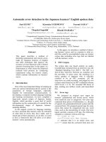
Figure 1: BER performance of the CDMA-BEM algorithm with
B
D
T
s
= 5·10
−3
, J = 4, N = 14, and K = 3. The BER performance
of the MLR and CDD is also shown for comparison.
In the following, we consider a four-user scenario (J = 4)
characterized by the matrix of signature cross-correlations
[43]:
R
4
=
1
7






7 −13 3
−17 3−1
337−1
3 −1 −17





. (38)
The BER performance of the CDMA-BEM receiver is il-
lustrated in Figure 1. Here it is assumed that the normal-
ized Doppler bandwith is B
D
T
s
= 5 · 10
−3
and that all the
users have the same SNR. In this figure the performance
of the maximum likelihood receiver (MLR) endowed w ith
ideal channel state information (CSI) and that of the co-
herent decorrelator detector (CDD) [47] are also shown for
comparison. It is interesting to note that, in these scenar-
ios, the CDMA-BEM almost achieves the same performance
of the MLR and outperforms the CDD by about 1.5 dB in

SNR.
Figure 2 shows the performance of CDMA-BEM versus
the normalized Doppler bandwidth for B
D
T
s
∈ (5·10
−3
,5·
10
−2
), under the assumption that SNR
j
= 15, 20, 25 dB for
j = 1, , 4. The error performance of the proposed algo-
rithm slightly worsens as the Doppler bandwidth increases
because of the poorer quality of the initial channel estimates.
Finally, the near-far resistance of the CDMA-BEM re-
ceiver is illustrated in Figure 3. The SNR of the first user
(SNR
1
) is set to 20 dB, whereas the other three SNRs (SNR
j
,
j = 2, 3, 4) are equal and vary in the range (5, 25) dB.
E
b
/N
0
= 15 dB

E
b
/N
0
= 20 dB
E
b
/N
0
= 25 dB
56789 2 3
4
5
0.01
B
D
T
s
0.001
0.01
0.1
BER
4
6
8
2
4
6
8
2

4
6
8
2
Figure 2: BER performance of the CDMA-BEM algorithm versus
B
D
T
s
. J = 4, E
b,k
/N
0
= 20 dB, N = 14, and K = 3.
MLR, user 1
MLR, users 2–4
CDMA-BEM, user 1
CDMA-BEM, users 2–4
510152025
E
b
/N
0
(dB)
0.001
0.01
0.1
BER
4
6

8
2
4
6
8
2
4
6
8
2
Figure 3: Near-far resistance of the CDMA-BEM algorithm. J = 4,
SNR
1
= 20 dB, SNR
k
∈ (5, 25) dB (k = 2, 3,4), and B
D
T
s
= 5·10
−3
.
The performance of the MLR is also shown for comparison.
These results show that, in this case, the CDMA-BEM ex-
hibits a perform ance which is substantially independent of
the energies of the interfering users.
Soft-In Soft-Output Detection 107
4.2. SISO detection of space-time block coded signals
4.2.1. Introduction
In the last years it has been shown that the information ca-

pacity of wireless communication systems can be substan-
tially increased by employing antenna arrays [48], jointly
with proper coding [49] and signal processing techniques
[50]. One of the most promising results in this research area
has been the development of new block and trellis codes for
multiple antennas, known as space-time codes (STCs) [49,
51]. Such codes provide significant diversity gains without
bandwidth expansion. Exact knowledge of the CSI is often
assumed in devising space-time decoding algorithms even
if channel estimation may represent a serious problem, es-
pecially in time-varying environments [52]. EM-based hard
detectors for STCs have been derived in [52, 53, 54]. In this
section a BEM-based soft detector for orthogonal STBCs is
illustrated.
4.2.2. Signal and channel models
Here we focus on a space-time block coded system employing
N
T
transmit and N
R
receive antennas [49]. The set of chan-
nel symbols transmitted during the nth block
4
is denoted
by the L × N
T
matrix S[n] = [s
l,i
[n]] (with l = 1, 2, , L,
i = 1, 2, , N

T
), where L is the overall duration of the block
in channel symbols and s
l,i
[n] is the channel symbol feeding
the ith antenna in the symbol interval (l + nL).
In the fol low ing we assume that the multiple channels
involved in the communication system are (a) affected by
frequency-flat Rayleigh fading and (b) quasi-static, that is,
channel variations within each block are negligible, whereas
changes from block to block are taken into account. Then the
path gain a
i, j
[n](withi = 1, 2, , N
T
and j = 1, 2, , N
R
)
from the ith transmit antenna to the jth receive antenna
during the nth block is a complex Gaussian random pro-
cess having zero mean and correlation function R
a
[m]
.
=
E{a
i, j
[n + m]a
∗
i, j

[n]} (with R
a
[0] = 1). Moreover, the gain
processes {a
i, j
[n]} are independent (rich scatterer environ-
ment).
Let r
l, j
[n] denote the received signal sample taken at the
output of the jth receive antenna in the (l + nL)th symbol
interval, with j = 1, , N
R
and l = 1, , L. Then the L × N
R
received signal matrix R[n] = [r
l, j
[n]] is given by [52]
R[n] = S[n]A[n]+W[n]. (39)
Here S[n] ∈ Ω,whereΩ ={S
m
, m = 1, , M} is an M-ar y
alphabet of unitary matrices (i.e., (S
m
)
H
S
m
= I
N

T
,whereI
n
is
the n×n identity matrix) [49, 51]. Moreover A[n] = [a
i, j
[n]]
and W[n] = [w
l, j
[n]] are the N
T
× N
R
fading matrix and the
L × N
R
noise matrix, respectively. The elements {w
l, j
[n]} of
W[n] are independent Gaussian random variables, all having
zero mean and variance σ
2
w
= 2N
0
.
4
Throughout the section, the parameter n denotes the block index,
whereas k specifies the location of a channel symbol within each block.
AsetofN consecutive vectors (39)(withn = 0, , N −

1) can be grouped as R
.
= [R
H
[0], R
H
[1], , R
H
[N − 1]]
H
((A)
T
and (A)
H
denote transpose and conjugated transpose
of A,resp.),with
R = D(S)A + W, (40)
where A
.
= [A
H
[0], A
H
[1], , A
H
[N − 1]]
H
and W
.
=

[W
H
[0], W
H
[1], , W
H
[N − 1]]
H
,respectively,andD( S)
.
=
diag{S[0], S[1], , S[N − 1]}.
4.2.3. A BEM-based SISO algorithm for space-time
block coded systems
Following the same indications illustrated in the previous ap-
plication, we set Θ = A and C ={R, S} in applying the BEM
technique. Then the auxiliary function is (analytical details
can be found in [55])
Q

A,
˜
A

=−
N
R

j=1
A

H
j

C
−1
A
+

1
σ
2
w

I
NN
T

A
j
−

2
σ
2
w

Re

˜
V

j
H
A
j

,
(41)
where A
j
is the jth column of A, C
A
.
= E{A
j
A
H
j
} is a fading
covariance matrix, and
˜
V
j
is the jth column of the matrix
˜
V
.
= D
H

˜

S

R (42)
with
˜
S ={
˜
S[n], n = 0, 1, N − 1}.Here
˜
S[n] =

S
m
∈Ω
S
m
Pr

S[n] = S
m


R,
˜
A

, (43)
where Pr(S[n] = S
m
|R,

˜
A) is the APP of the event {S[n] =
S
m
},givenR and A =
˜
A. Starting from (41), the follow-
ing BEM-based recursive channel estimator can be derived.
Given the channel estimate A
(k)
at the kth iteration, the next
estimate A
(k+1)
is evaluated as
A
(k+1)
j
= [P]
−1
V
(k)
j
, (44)
where P
.
= I
NN
T
+ σ
2

w
C
−1
A
. The APPs {Pr(S[n] = S
m
|R,
˜
A)}
needed for the evaluation of (42) can be computed using the
Bayes formula
Pr

S[n] = S
m


R,
˜
A

=
f

R[n]


S
m
,

˜
A[n]

Pr

S
m


˜
S
m
∈Ω
f

R[n]


˜
S
m
,
˜
A[n]

Pr

˜
S
m


,
(45)
where Pr(S
m
) is the probability of the event {S[n] = S
m
},and
f

R[n]


S
m
,
˜
A[n]

=
1
det

πσ
2
w
I
L

N

R
exp

−
h

R[n], S
m
,
˜
A[n]

σ
2
w

(46)
with h(R[n], S
m
,
˜
A[n])
.
= tr{(R[n] − S
m
˜
A[n])
H
(R[n] −
S

m
˜
A[n])}.
108 EURASIP Journal on Wireless Communications and Networking
It is important to note that (a) P does not depend on the
index of the receive antenna; (b) the inverse of P does not
need to be recomputed as long as the channel statistics do
not change; (c) (44) can be simplified factoring C
A
as
C
A
=
˜
C
a
⊗ I
N
T
, (47)
where
˜
C
a
is the covariance matrix of the vector a
i, j
=
[a
i, j
[0], a

i, j
[1], , a
i, j
[N −1]]
T
and ⊗ is the Kronecker prod-
uct, so that P = (I
N
+ σ
2
w
˜
C
−1
a
) ⊗ I
N
T
.
After K iterations the BEM algorithm stops producing
a channel estimate A
BEM
= A
(K)
and the APPs {Pr(S[n] =
S
m
|R, A
BEM
)} which can be processed exactly like in the pre-

vious application. In the following the BEM-based estima-
tion algorithm (43)–(46) is dubbed STBC-BEM.
4.3. Numerical results
The error performance of the STBC-BEM algorithm has
been assessed by computer simulation for the Alamouti’s
space-time block code [51]. Then we have
S[n]
.
=

s
1
n
s
2
n
−

s
2
n

∗

s
1
n

∗


, (48)
where the symbols {s
1
n
, s
2
n
} belong to a BPSK constellation.
5
In the following we assume that (1) R
a
[m] = J
0
(2πmLB
D
T),
where J
0
(x) is the zeroth-order Bessel function of the first
kind, B
D
is the fading Doppler bandwidth, and T is the sig-
naling interval; (2) the SNR is defined as E
b
/N
0
,whereE
b
is
the average received energy per receive antenna and informa-

tion bit; (3) each packet of (N
B
− 1) consecutive information
blocks is followed by one pilot block, so that the pilot symbol
rate is R
p
= 1/N
B
.
The STBC-BEM algorithm processes a sample set R con-
sisting of N · L consecutive received signal samples, corre-
sponding to N transmitted symbol blocks. It is assumed that
the first and last L samples of R always correspond to a pi-
lot block. This entails that (a) N = N
p
N
B
+1,ifN
p
packets
are processed, and (b) the last block of each set is in com-
mon with the first of the next one. The information provided
by the pilot symbols is exploited to initialize the BEM algo-
rithm. In particular the initial channel estimate for the jth
receive antenna is evaluated as A
j
= FR
j
,whereR
j

is the
jth column of R,withj = 1, 2, , N
R
.HereF is an opti-
mal NN
T
× NLmatrix that can be easily derived by standard
methods (Wiener filtering) [29, 36], under the assumptions
that (a) the information channel symbols are independent
and identically distributed and (b) the pilot symbols are ex-
actly known.
In all the following results it is assumed that the BEM
algorithm processes N
p
= 4 consecutive packets, each con-
sisting of N
B
= 10 consecutive blocks.
5
Further results (not shown for space limitations) evidence that the com-
ments expressed for a BPSK system also apply to larger constellations.
Coherent
BEM and WF
ML and WF
ML and LMS
0 5 10 15 20 25
E
b
/N
0

10
−6
10
−5
10
−4
10
−3
10
−2
10
−1
10
0
BER
Figure 4: BER performance of various detection algorithms with
Alamouti’s STBC. N
R
= 1andB
D
T = 2·10
−2
.
In Figure 4 the error performance of the STBC-BEM
(with K = 3) is compared with that provided by an ML re-
ceiver using WF channel estimation
6
and an ML receiver us-
ing decision-directed least mean square (LMS) channel track-
ing w ith step size µ = 0.5 (the tracker is initialized for each

packet using the pilot block at its beginning in order to avoid
runaway problems) for single receive diversity (N
R
= 1) and
B
D
T = 2·10
−2
. The BER performance of a coherent receiver
endowed with ideal CSI is also shown. These results evidence
that (1) since the energy loss due to pilot symbols is 0.45 dB,
the BEM performs very well if the fading rate is not too large;
(2) the BEM substantially outperforms the other detectors.
Further simulations have also shown that a blind SISO de-
tector based on the EM-based approach illustrated in [6]and
initialized by a WF does not outperform the ML detector en-
dowed with the same channel estimator.
Figure 5 shows the error performance of the STBC-BEM
with a different number of iterations, that is, with K = 1,
2, and 3, in the same scenario as the previous figure. These
results evidence the usefulness of running three full iterations
in the BEM procedure, in order to approach the performance
of a coherent receiver endowed with ideal CSI. We also found,
however, that negligible gains are offered by K>3.
The comments already expressed about the results of
Figure 4 also apply to Figure 6, referring to double receive
diversity (N
R
= 2), channel estimation based on WF and
B

D
T = 5·10
−3
,10
−2
,and2·10
−2
for the BEM (B
D
T =
2·10
−2
only is considered for the ML detector). This figure
6
Its error performance coincides with that offered by the BEM without
iterations.
Soft-In Soft-Output Detection 109
Coherent
BEM, 1st iter.
BEM, 2nd iter.
BEM, 3rd iter.
0 5 10 15 20 25
E
b
/N
0
10
−5
10
−4

10
−3
10
−2
10
−1
BER
Figure 5: BER performance of the BEM detection algorithm with
Alamouti’s STBC. The error performance of the coherent detector
is also shown for comparison. N
R
= 1, B
D
T = 2·10
−2
,andK = 1,
2, and 3.
also evidences that the BEM performance is not substan-
tially affected by a change in the Doppler rate, provided that
B
D
T ≤ 2·10
−2
.
In Figure 7 the BEM and the ML detector BER versus the
normalized Doppler bandwidth B
D
T is shown for B
D
T ∈

(10
−2
,5·10
−2
)andE
b
/N
0
= 10dB(WFisusedinbothcases).
It is worth noting that the performance degradation increases
for larger Doppler bandwidths as the quality of the initial es-
timate of the BEM becomes poorer and this prevents BEM
convergence to the global maximum, at least over some data
blocks. Simulation results have also evidenced that, in this
case, increasing the number of BEM iterations provides a
negligible improvement.
4.4. SISO detection of space-time
block coded OFDM signals
4.4.1. Introduction
The use of OFDM is often suggested to simplify channel
equalization in the presence of appreciable frequency se-
lectivity. When employed in MIMO w ireless systems, the
OFDM technique can be also easily combined w ith channel
codes devised for multiple tr a nsmit antennas, that is, with
space-time (ST) codes. A further improvement in the sys-
tem performance can be achieved when conventional outer
channel codes, like convolutional codes [56, 57]orlow-density
parity-check (LDPC) codes [58], are used in conjunction with
proper ST symbol mappers.
Decoding of ST codes usually requires an accurate knowl-

edge of CSI at the receiver. In MIMO OFDM systems, how-
ever, channel estimation may represent a serious problem,
Coherent
BEM, B
D
T = 5 · 10
−3
BEM, B
D
T = 10
−2
BEM, B
D
T = 2 · 10
−2
ML, B
D
T = 2 · 10
−2
02468101214
E
b
/N
0
10
−5
10
−4
10
−3

10
−2
10
−1
BER
Figure 6: BER performance of various detection algorithms with
Alamouti’s STBC. N
R
= 2.
especially in time-varying environments, because of the high
complexity needed to achieve a satisfying accuracy [59], even
if simplified pilot-based channel estimators can be devised
[60]. Recently, it has been shown that, when OFDM is com-
bined with ST block coding [51] and a pilot-based channel
estimate is available at the receiver, the EM technique can be
applied to devise accurate channel estimators [61] and that
such estimators can be used for soft-in hard-output detection
[54]. In the last case, hard decisions are then converted to soft
data information which can be exploited in iterative receiver
architectures when outer coding is employed at the transmit-
ter. In this part we tackle the same problem, but from a dif-
ferent perspective. In fact, we derive a SISO module based
on the BEM technique. Preliminary simulation results sug-
gest that this algorithm offers better performance than that
derived in [54] with a lower overall computational burden.
4.4.2. Signal and channel models
In this paper we consider an ST block coded OFDM system
employing N subcarriers jointly with N
T
transmit and N

R
receive antennas. The block diagram of the communication
system is illustrated in Figure 8a. The coding scheme results
from the concatenation of a convolutional or an LDPC code
with an orthogonal STBC. It is worth noting that that LDPC
codeshavesomerelevantproperties[62], like low decoding
complexity and excellent performance, which make them a
promising coding technique for ST coded OFDM systems
[58].
The input bit stream is partitioned into blocks, each in-
dependently encoded by means of a channel encoder. After
(optional) bit interleaving (Π) the coded bits are mapped
110 EURASIP Journal on Wireless Communications and Networking
Coherent, N
R
= 1
Coherent, N
R
= 2
BEM, N
R
= 1
BEM, N
R
= 2
ML, N
R
= 1
ML, N
R

= 2
56789 2 3 4 56789
0.01 0.1
B
D
T
10
−6
10
−5
10
−4
10
−3
10
−2
10
−1
BER
Figure 7: BER versus the normalized Doppler bandwidth B
D
T for
various detection algorithms with STBC. E
b
/N
0
= 10 dB. N
R
= 1
and 2.

into channel symbols belonging to an M-ary PSK constel-
lation. The resulting symbol sequence feeds an ST orthog-
onal block encoder. In the following, we consider, for sim-
plicity, the Alamouti’s STBC [51], even if the proposed de-
tection algorithm can be easily extended to any orthogonal
ST block code. The output sequence of the ST encoder is
passed through a bank of N
T
inverse dis crete Fourier trans-
form (IDFT) processors, which generate an ST-OFDM code-
word spanning L OFDM symbol intervals. For instance, with
Alamouti’s STBC, we have L = 2 and, if c
0
[l, n]andc
1
[l, n]
denote the channel symbols transmitted on the nth OFDM
subcarrier (with n = 0, , N − 1) in the lth OFDM sym-
bol interval (with l even) by the first and the second trans-
mit antenna, respectively, then c
0
[l +1,n] =−c
∗
1
[l, n]and
c
1
[l +1,n] = c
∗
0

[l, n] are sent in the next symbol interval. In
other words, the resulting codeword associated with the nth
subcarrier is represented by the matrix
S[n] =

c
0
[l, n] c
1
[l, n]
c
0
[l +1,n] c
1
[l +1,n]

(49)
belonging to an alphabet Ω ={S
p
, p = 1, , P} (with P =
M
2
) of unitary matrices [51].
The OFDM signal is transmitted over a wide sense sta-
tionary uncorrelated scattering (WSS-US) MIMO channel
[63]. In the following it is assumed that (a) all the single-
input single-output channels associated with different trans-
mit/receive antenna pairs are mutually independent, iden-
tically distributed and are affected by Rayleigh fading; (b)
in the propagation scenario, frequency dispersion i s inde-

pendent of time dispersion. Under these hypotheses a full
statistical description of the MIMO channel is provided by
its power delay profile (PDP) and its Doppler power de nsity
spectrum (PDS) or, equivalently, by its frequency correlation
function R
H
( f ) and its time correlation function R
D
(t), re-
spectively [63]. At the receiver (see Figure 8b)abankofN
R
DFT processors (one per receive antenna) is fed by N
R
dis-
tinct discrete-time signal sequences produced by matched-
filtering and symbol-rate sampling. T he outputs of the DFTs
are processed by a BEM-based SISO detection algorithm
(see the following paragraph) operating on a codeword-by-
codeword basis. For this reason, in the following, we con-
centrate on the detection of a single ST-OFDM codeword. In
particular, if r
j
[l, n] denotes the received signal sample taken
at the output of the jth DFT for the nth subcarrier frequency
in the lth OFDM symbol interval, with j = 0, 1, , N
R
− 1
and n = 0, , N − 1, we always take a couple of consecu-
tive received signal samples for l = 0, 2, 4, If we assume
that the fading process remains constant over an ST code-

word (i.e., over two adjacent OFDM symbol intervals with
Alamouti’s STBC), the L × N
R
matrix R[l, n] = [r
j
[l, n]] col-
lecting the received signal samples over the observation in-
terval for the nth subcarrier can be expressed as [54]
R[l, n] = S[l, n]H[l, n]+W[l, n]. (50)
Here, S[n, l] is the L × N
T
transmitted codeword matrix (see
(49)), H[l, n] = [H
i, j
[l, n]] is an N
T
× N
R
channel response
matrix (H
i, j
[l, n] represents the complex channel gain be-
tween the ith transmit and the jth receive antenna at the nth
subcarrier frequency), and W[l, n] = [w
l, j
[l, n]] is an L × N
R
noise matrix. The elements {w
l, j
[l, n]} of W[l, n] are inde-

pendent complex zero mean Gaussian random variables with
variance σ
2
w
= 2N
0
. We also note that {H
i,j
[l, n]} are com-
plex Gaussian random variables with zero mean and that the
correlation between H
i, j
[l, n + m]andH
i, j
[l, n]isgivenby
R
H
[m] = E{H
i, j
[l, n + m]H
∗
i, j
[l, n]}=R
H
(mf
∆
), where f
∆
is
the subcarrier spacing.

For a given l, the matr ices (50) associated with all the dif-
ferent subcarriers (n = 0, , N − 1) can be grouped in an
LN×N
R
matrix R[l]
.
= [R
H
[l,0],R
H
[l,1], , R
H
[l, N−1]]
H
.
If the dependence on l is dropped, for simplicity, this vector
can be expressed as
R = D(S)H + W, (51)
where H
.
= [H
H
[0], H
H
[1], , H
H
[N − 1]]
H
, W
.

= [W
H
[0],
W
H
[1], , W
H
[N − 1]]
H
,andD(S)
.
= diag{S[0], S[1], ,
S[N − 1]}.
4.4.3. A BEM-based SISO algorithm for OFDM systems
Following the same approach as the previous two scenarios,
we choose Θ = H and I = S. Then, as shown in [35], the
BEM auxiliary function (6) can be expressed as
Q

H,
˜
H

=−
N
R

j=1
H
H

j
MH
j
−
2
σ
2
w
Re

˜
V
H
j
H
j

, (52)
Soft-In Soft-Output Detection 111
Data in
Outer
encoder

Symbol
mapper
Space-time
block encoder
.
.
.

OFDM
modulator
OFDM
modulator
(a)
Data out
Outer SISO
decoder
Π
−1
Bit metric
computation
I
(2)
d,i
[k] I
(1)
d,e
[k]
+
+
−
I
(1)
d,o
[k]
ST-OFDM
BEM
R
A

0
R
Buffer
.
.
.
OFDM
demodulation
OFDM
demodulation
Π
STBC metric
computation
I
(2)
d,o
[k]+
+
− I
(2)
d,e
[k] I
(1)
d,i
[k]
BEM
initialization
Π
STBC metric
computation

I
(2)
d,o
[k]
k = 0
(b)
Figure 8: Block diagrams of the space-time block coded OFDM: (a) transmitter and (b) receiver.
where H
j
is the jth column of the matrix H, M
.
= C
−1
H
+
(1/σ
2
w
)I
NI
with C
H
= E{H
j
H
H
j
},
˜
V

j
is the jth column of the
matrix
˜
V
.
= D
H
(
˜
S)R, and the matrix
˜
S results from the or-
dered concatenation of the matrices {
˜
S[n], n = 0, 1, ,N −
1},with
˜
S[n]
.
=

S
m
∈Ω
S
m
Pr

S[n] = S

m


R,
˜
H

. (53)
The APPs
{Pr(S[n] = S
m
|R,
˜
H)} can be evaluated using the
Bayes formula
Pr

S[n] = S
m


R,
˜
H

=
f

R[n]



S
m
,
˜
H[n]

P

S
m


˜
S
m
∈Ω
f

R[n]


˜
S
m
,
˜
H[n]

P


˜
S
m

,
(54)
where
f

R[n]


S
m
,
˜
H[n]

= C
R
exp

−
h

R[n],S
m
,
˜

H[n]

σ
2
w

(55)
with C
R
.
= det(πσ
2
w
I
L
)
−N
R
and h(R[n], S
m
,
˜
H[n])
.
= tr{(R[n]
− S
m
˜
A[n])
H

· (R[n] − S
m
˜
A[n])
}. The BEM algorithm oper-
ates as follows. Given the channel estimate H
(k)
at the kth
iteration, the next estimate H
(k+1)
is evaluated as
H
(k+1)
j
= P
−1
V
(k)
j
(56)
with P
.
= I
NN
T
+ σ
2
w
C
−1

H
and j = 1, 2, , N
R
.Itisimportant
to note that (a) P does not depend on the index of the receive
antenna; (b) the inverse of P does not need to be recomputed
as long as the channel statistics do not change; (c) (56)can
be simplified factoring C
H
as
C
H
=
˜
C
H
⊗ I
N
T
, (57)
where
˜
C
H
is the covariance matrix of the vector H
i, j
=
[H
i, j
[0], H

i, j
[1], , H
i, j
[N − 1]]
T
and ⊗ is the Kronecker
product, so that P = ( I
N
+ σ
2
w
˜
C
−1
H
) ⊗ I
N
T
. In the following
the BEM-based estimation algorithm (53)–(56)isdubbed
ST-OFDM BEM.
After K iterations the BEM algorithm stops producing a
channel estimate H
BEM
= H
(K)
and the APPs {Pr(S[n] =
S
m
|R, H

BEM
)}. These can be exploited to take MAP deci-
sions or for soft decoding of an outer code in a concate-
nated scheme. In our work, we have considered the iter-
ative receiver structure as shown in Figure 8b. This struc-
ture operates as follows. After OFDM demodulation, the ST-
OFDM BEM module takes as input the received signal vector
R
.
= [R
H
[0], R
H
[1], , R
H
[N − 1]]
H
, an initial channel esti-
mate matrix H
(0)
(consisting of N ·N
T
×N
R
matrices H
(0)
[n])
and the N × P a priori information matrices {I
l(1)
d,i

[k] =
[(I
l(1)
d,i
[k])
n,m
]}.Here(I
l(1)
d,i
[k])
n,m
= log Pr
(l)
(S[n] = S
m
),
where Pr
(l)
(S[n] = S
m
) denotes the APRP that S[n]is
equal to the mth codeword of the alphabet Ω at the
kth step. After K iterations the BEM algorithm produces
112 EURASIP Journal on Wireless Communications and Networking
the N × P output matrices {I
l(1)
d,o
[k] = [(I
l(1)
d,o

[k])
n,m
]}
with (I
l(1)
d,o
[k])
n,m
= log Pr
(l)
(S[n] = S
m
|R, H
BEM
), where
Pr
(l)
(S[n] = S
m
|R, H
BEM
) represents the APP of the event
{S[n] = S
m
} at the kth step. Then the extrinsic information
matrices {I
l(1)
d,e
[k]} are evaluated as I
l(1)

d,e
[k] = I
l(1)
d,o
[k]−I
l(1)
d,i
[k].
Since interleaving is performed at the bit level, before send-
ing the extrinsic information to the deinterleaver (Π
−1
)and
to the SISO decoder, the evaluation of the soft bit metrics is
needed (see [64, Section II-C]). The channel decoder pro-
duces the a posteriori bit information matrices and, after bit
interleaving and probability recombination, the a posteriori
symbol information matrices {I
l(2)
d,o
[k]} (in log form). Finally,
at the last iteration, the SISO decoder computes the APP
matrix {P
b
} together with a bit estimate vector. Subtracting
{I
l(2)
d,i
[k]} from {I
l(2)
d,o

[k]} produces the extrinsic information
matrices {I
l(2)
d,e
[k]} of the channel symbols which are fed back
as input to the ST-OFDM BEM decoder.
In our simulations both convolutional and LDPC codes
have been employed. With convolutional codes the bit APRPs
produced by the ST-OFDM BEM feed a Bahl Cocke Jelinek
Raviv (BCJR) algorithm [20] implemented in its log MAP
form [65]. With LDPC codes bit log-likelihood ratios (LLRs)
are evaluated on the basis of the bit APRPs and sent to an
LDPC decoder based on the belief propagation (BP) algo-
rithm [62, 66 ]. It is important to point out that (a) the par-
ity check matrices of the LDPC codes employed in our work
have been generated in a random fashion [67], avoiding cy-
cles of length 4 in the code graph in order to improve the code
distance properties; (b) due to the random generation of the
encoding matrix, no external interleaver (deinterleaver) is
needed at the output (input) of the LDPC encoder (decoder)
[58].
Finally, we note that, in the proposed receiver structure,
the APPs {I
l(2)
d,o
[k]}, after interleaving, are also used to eval-
uate the estimate H
(k+1)
needed for the initialization of the
ST-OFDM BEM in the (k + 1)th iteration of the receiver. At

the beginning of the first iteration, however, no aprioriin-
formation on the channel symbols is available. For this rea-
son the initial fading estimate H
(0)
of the ST-OFDM BEM
is evaluated by means of the pilot-based channel estimation
algorithm derived in [60].
4.5. Numerical results
In this paragraph some BER results are illustrated. In our
computer simulations the reduced complexity model for
WSS-US channels proposed in [68] has been used for the
generation of a MIMO multipath fading channel. In particu-
lar, for a given Doppler bandwidth B
D
, the Doppler PDS has
been defined as S
D
( f ) = 1 − 1.72 f
2
0
+0.785 f
4
0
for f
0
≤ 1
and S
D
( f ) = 0for f
0

> 1, where f
0
= f/B
D
[69]. More-
over, the multipath MIMO channel has been modeled as a
3-tap delay line approximating an exponential PDP P
h
(τ) =
τ
−1
0
exp(−τ/τ
0
)u(τ), with τ
0
= 1.56 microseconds (the corre-
sponding frequency correlation function is R
H
( f ) = 1/(1 +
j2πfτ
0
)). Then, in accordance with the OFDM physical
layer specifications for the broadband radio access networks
(BRAN) in [70], the following parameters have been selected
for the ST block coded OFDM system: (a) the DFT order
is N
= 256; (b) the number of useful OFDM subcarriers
is equal to 192, since the total number of subcarriers N in-
cludes 27 suppressed carriers on the upper frequencies, 28

suppressed carriers on the lower frequencies, 8 BPSK pilot
symbols, and 1 DC carrier set to 0; (c) the OFDM symbol in-
terval is T
S
= 0.125 microseconds; (d) the length of the cyclic
prefix in the OFDM modulator has been set to 64; (d) with
convolutional codes, a 4-state rate 1/2 convolutional code
with generators g
1
= (5)
8
and g
2
= (7)
8
has been adopted,
when used; (e) with LDPC codes, a regular (3,6) code with
rate R = 1/2 and a BP a lgorithm with a maximum num-
ber of iterations equal to 10 have been adopted, when used;
(f) QPSK modulation has been employed for both uncoded
and coded transmission; (g) a single frame consists of 9 ST
block coded OFDM information codewords plus one pilot
ST block coded OFDM codeword appended at its beginning.
Moreover a single receive antenna, that is, N
R
= 1anda
Doppler bandwidth B
D
= 200 Hz have been chosen for our
simulations.

In addition, the following assumptions have been made
at the receive side: (a) the SNR is defined as E
b
/N
0
,whereE
b
is the average captured energy per receive antenna and in-
formation bit; (b) the BEM algor ithm processes a block con-
sisting of 192 Alamouti’s space-time block codewords, and
accomplishes K = 3 complete iterations; (c) the last channel
estimate generated by the the BEM algorithm for each ST-
OFDM codeword is used as an initial estimate of the same
algorithm for the next codeword.
Figure 9 shows the ST-OFDM BEM algorithm perfor-
mance without outer channel coding. Comparison is made
with an ML detector endowed with ideal CSI (genie bound)
and with an ML detector endowed with the same pilot-based
channel estimator (CE) as the BEM [60]. These results evi-
dence that the ST-OFDM BEM algorithm substantially out-
performs a realistic ML detector. We also note that the energy
loss due to pilot symbol insertion is 0.45 dB, so that the en-
ergy gap between the genie bound and the ST-OFDM BEM
is about 1.5 dB [71].
Some simulation results referring to a convolutionally
encoded system are shown in Figure 10, comparing the BER
performance provided by the iterative receiver described in
the previous paragraph (with 0, 1, and 2 iterations) with that
offered by a BCJR decoder endowed with ideal CSI. We have
also considered a receiver structure in w hich the likelihoods

produced by the above-mentioned ML detector with pilot-
based CE are exploited to generate soft data information
feeding, after deinterleaving, the SISO outer decoder. The
proposed iterative architecture substantially outperforms the
latter and, if the energ y loss due to pilot symbols is neglected,
it approaches closely the genie bound. It is also worth not-
ing that, in this scenario, carrying out global iterations pro-
vides a very small gain. This result can be explained as fol-
lows. The ST-OFDM BEM, starting from a pilot-based chan-
nel estimate, produces a good channel estimate and a good
estimate of the data APPs since the beginning, that is, even
in the absence of the APRPs produced by the BCJR, despite
Soft-In Soft-Output Detection 113
Genie bound
ML with CE
ST-OFDM BEM
024681012
E
b
/N
0
0.1
BER
2
3
4
5
6
7
8

9
2
Figure 9: BER performance of the ST-OFDM BEM algorithm with-
out outer coding. N
R
= 1andK = 3.
Genie bound
ML with CE
ST-OFDM BEM
ST-OFDM BEM, iter. 1
ST-OFDM BEM, iter. 2
024681012
E
b
/N
0
0.001
0.01
0.1
BER
Figure 10: BER performance of the ST-DFDM BEM iterative re-
ceiver. Convolutional coding, N
R
= 1, and K = 3.
the appreciable Doppler rate. These results are substantially
different than those illustrated in [54, page 223], evidencing,
for instance, a strong gap between the performance in the ab-
sence of iterations and that achieved after one iteration and
suggesting the use of 3–5 global iterations. On the basis of
these preliminary results, since the complexity (per iteration)

Genie bound
ML with CE
ST-OFDM BEM
024681012
E
b
/N
0
0.001
0.01
0.1
BER
Figure 11: BER performance of the ST-OFDM BEM receiver. LDPC
coding, N
R
= 1, and K = 3.
of the ST-OFDM BEM and that of the EM algorithm derived
in [54] are comparable, the use of the former should be pre-
ferred to the latter, since it ensures faster convergence, that is,
a smaller overall complexity.
Finally, in Figure 11 the performance of the ST-OFDM
BEM receiver for LDPC-coded signals is illustrated. The BER
performance of the proposed algorithm is compared with
that obtained by a BP algorithm endowed with perfect CSI.
The curve labeled as “ML with CE” represents the BER per-
formance of an ML detector endowed with pilot-based CE
and followed by the LDPC decoder. Even without turbo de-
coding , the ST-OFDM BEM algorithm brings a substantial
gain against the ML-based symbol detection approach. It is
worth noting that, in this scenario, the BER performances

given by the LDPC and convolutional coding schemes are
widely comparable. This poor behavior obtained by LDPC
coding is mainly due to the small dimension of the parity-
check matrix employed in our simulations.
5. CONCLUSIONS
In this paper the BEM technique has been proposed to solve
MAP estimation problems. In particular, we have shown that
it represents a useful tool to derive novel SISO detectors
for communication channels with random parametric un-
certainty and memory. As an application of these concepts,
SISO modules for the iterative detection of coded digital sig-
nals transmitted over fading channels have been derived in
three specific scenarios and their error performance has been
assessed. Applications of the BEM technique to other com-
munication scenarios are the subject of ongoing research ac-
tivities.
114 EURASIP Journal on Wireless Communications and Networking
ACKNOWLEDGMENTS
This work has b een performed in the framework of the
project STINGRAY IST-2000-30173, which is funded by the
European Community. The authors would like to acknowl-
edge the contributions of their colleagues from the Intracom
Hellenic Telecommunications and Electronics Industry S.A.,
the University of Modena and Reggio Emilia, the Institute
of Accelerating Systems and Applications, the Technical Re-
search Centre of Finland, and the National Technical Univer-
sity of Athens.
REFERENCES
[1] D. P. Taylor, G. M. Vitetta, B. D. Hart, and A. M
¨

ammel
¨
a,
“Wireless channel e qualization,” European Transactions on
Telecommunications, vol. 9, no. 2, pp. 117–143, 1998.
[2] R. Raheli, A. Polydoros, and C K. Tzou, “Per-survivor pro-
cessing: a general a pproach to MLSE in uncertain environ-
ment,” IEEE Trans. Commun., vol. 43, no. 234, pp. 354–364,
1995.
[3] C. N. Georghiades and J. C. Han, “Sequence estimation in the
presence of random parameters via the EM algorithm,” IEEE
Trans. Commun., vol. 45, no. 3, pp. 300–308, 1997.
[4] H. Zamiri-Jafarian and S. Pasupathy, “Adaptive MLSDE using
the EM algorithm,” IEEE Trans. Commun.,vol.47,no.8,pp.
1181–1193, 1999.
[5] A. Anastasopoulos and K. M. Chugg, “Adaptive soft-input
soft-output algorithms for iterative detection with parametric
uncertainty,” IEEE Trans. Commun., vol. 48, no. 10, pp. 1638–
1649, 2000.
[6] G. K. Kaleh and R. Vallet, “Joint parameter estimation and
symbol detection for linear or nonlinear unknown channels,”
IEEE Trans. Commun., vol. 42, no. 7, pp. 2406–2413, 1994.
[7] G. K. Kaleh, “Joint carrier phase estimation and symbol de-
coding of trellis codes,” European Transactions on Telecommu-
nications, vol. 4, no. 2, pp. 157–163, 1993.
[8] C. A. Haro, J. A. R. Fonollosa, and J. Fonollosa, “Blind channel
estimation and data detection using hidden Markov models,”
IEEE Trans. Signal Processing, vol. 45, no. 1, pp. 241–247, 1997.
[9] W. Turin, “Map decoding in channels with memory,” IEEE
Trans. Commun., vol. 48, no. 5, pp. 757–763, 2000.

[10] L. Davis, I. Collings, and P. Hoeher, “Joint MAP equal-
ization and channel estimation for frequency-selective and
frequency-flat fast-fading channels,” IEEE Trans. Commun.,
vol. 49, no. 12, pp. 2106–2114, 2001.
[11]P.HoeherandJ.Lodge, “TurboDPSK:iterativedifferen-
tial DPSK demodulation and channel decoding,” IEEE Trans.
Commun., vol. 47, no. 6, pp. 837–843, 1999.
[12] I. D. Marsland and P. T. Mathiopoulos, “Multiple differen-
tial detection of parallel concatenated convolutional (turbo)
codes in correlated fast Rayleigh f ading,” IEEE J. Select. Areas
Commun., vol. 16, no. 2, pp. 265–274, 1998.
[13] M. J. Gertsman and J. H. Lodge, “Symbol-by-symbol MAP
demodulation of CPM and PSK signals on Rayleigh flat-
fading channels,” IEEE Trans. Commun.,vol.45,no.7,pp.
788–799, 1997.
[14] J. Hagenauer, “The turbo principle: tutorial introduction and
state of the art,” in Proc. International Symposium on Turbo
Codes & Related Topics, pp. 1–11, Brest, France, September
1997.
[15] J. Hagenauer, E. Offer, and L. Papke, “Iterative decoding of
binary block and convolutional codes,” IEEE Trans. Inform.
Theory, vol. 42, no. 2, pp. 429–445, 1996.
[16] B. Sklar, “A primer on turbo code concepts,” IEEE Commun.
Magazine, vol. 35, no. 12, pp. 94–102, 1997.
[17] C. Berrou and A. Glavieux, “Near optimum error correcting
coding and decoding: turbo-codes,” IEEE Trans. Commun.,
vol. 44, no. 10, pp. 1261–1271, 1996.
[18] S. Benedetto, D. Divsalar, G. Montorsi, and F. Pollara, “A soft-
input soft-output APP module for iterative decoding of con-
catenated codes,” IEEE Communications Letters, vol. 1, no. 1,

pp. 22–24, 1997.
[19] Y. Lin, B. Vucetic, and Y. Sato, “Optimum soft-output detec-
tion for channels with intersymbol interference,” IEEE Trans.
Inform. Theory, vol. 41, no. 3, pp. 704–713, 1995.
[20] L. R. Bahl, J. Cocke, F. Jelinek, and J. Raviv, “Optimal decoding
of linear codes for minimizing symbol error rate (Corresp.),”
IEEE Trans. Inform. Theory, vol. 20, no. 2, pp. 284–287, 1974.
[21] V. Franz and J. B. Anderson, “Concatenated decoding with a
reduced-search BCJR algorithm,” IEEE J. Select. Areas Com-
mun., vol. 16, no. 2, pp. 186–195, 1998.
[22] S. Benedetto, G. Montorsi, D. Divsalar, and F. Pollara, “Soft-
input, soft-output modules for the construction and dis-
tributed iterative decoding of code networks,” European
Transactions on Telecommunications, vol. 9, no. 2, pp. 155–
172, 1998.
[23] C. Douillard, A. Picart, M. J
´
ez
´
equel, P. Didier, C. Berrou, and
A. Glavieux, “Iterative correction of intersymbol interference:
turbo-equalization,” European Transactions on Telecommuni-
cations, vol. 6, no. 5, pp. 507–511, 1995.
[24] A. P. Dempster, N. M. Laird, and D. B. Rubin, “Maximum
likelihood from incomplete data via the EM algorithm,” Jour-
nal of the Royal Statist ical Society: Series B,vol.39,no.1,pp.
1–38, 1977.
[25] T. K. Moon, “The expectation-maximization algorithm,”
IEEE Signal Processing Mag., vol. 13, no. 6, pp. 47–60, 1996.
[26] H. Z. Jafarian and S. Pasupathy, “Em-based recursive estima-

tion of channel parameters,” IEEE Trans. Commun., vol. 47,
no. 9, pp. 1297–1302, 1999.
[27] V. Lottici and M. Luise, “Embedding carrier phase recovery
into iterative decoding of turbo-coded linear modulations,”
IEEE Trans. Commun., vol. 52, no. 4, pp. 661–669, 2004.
[28] N. Noels, C. Herzet, A. Dejonghe, et al., “Turbo synchroniza-
tion: an EM algorithm interpretation,” in Proc. IEEE Inter-
national Conference on Communications (ICC ’03), pp. 2933–
2937, Anchorage, Alaska, USA, May 2003.
[29] E. Chiavaccini and G. M. Vitetta, “MAP symbol estimation in
the presence of random parameters via a generalized EM al-
gorithm,” in Proc. IEEE International Conference on Commu-
nications (ICC ’01), vol. 4, pp. 1057–1061, Helsinki, Finland,
June 2001.
[30] E. Chiavaccini and G. M. Vitetta, “A BEM-based detector for
CPM signals transmitted over frequency-flat fading channels,”
IEEE Transactions on Wireless Communications,vol.2,no.3,
pp. 409–412, 2003.
[31] E. Chiavaccini and G. M. Vitetta, “MAP symbol estimation
on frequency-flat Rayleigh fading channels via a Bayesian EM
algorithm,” IEEE Trans. Commun., vol. 49, no. 11, pp. 1869–
1872, 2001.
[32] E. Chiavaccini and G. M. Vitetta, “A per-survivor phase-
estimation algorithm for detection of PSK signals,” IEEE
Trans. Commun., vol. 49, no. 12, pp. 2059–2061, 2001.
[33] A. S. Gallo, E. Chiavaccini, and G. M. Vitetta, “BEM-based
multiuser detection for synchronous DS-CDMA systems over
frequency flat fading channels,” in Proc. 13th IEEE Interna-
tional Symposium on Personal, Indoor and Mobile Radio Com-
munication Conference (PIMRC ’02), vol. 3, pp. 1285–1289,

Lisbon, Portugal, September 2002.
[34] E. Chiavaccini, A. S. Gallo, and G. M. Vitetta, “BEM-Based
SISO detection of space-time block coded signals transmit-
ted over frequency-flat fading channels,” in Proc. IEEE Global
Soft-In Soft-Output Detection 115
Telecommunications Conference (GLOBECOM ’02), vol. 1, pp.
374–378, Taipei, Taiwan, November 2002.
[35] A.S.GalloandG.M.Vitetta, “Anovelsoft-insoft-outdetec-
tion algorithm for space-time concatenated coding schemes
operating over multipath fading channels,” submitted to the
IEEE Global Te lecommunications Conference (GLOBECOM
’04), 2004.
[36] C. W. Helstrom, Elements of Signal Detection & Estimation,
Prentice-Hall, Englewwod Cliffs, NJ, USA, 1995.
[37] A. Gelman, J. B. Carlin, H. S. Stern, and D. B. Rubin, Bayesian
Data Analysis, Chapman & Hall, London, UK, 1995.
[38] G. M. Vitetta, D. P. Taylor, and U. Mengali, “Double-filtering
receivers for PSK signals transmitted over Rayleigh frequency-
flat fading channels,” IEEE Trans. Commun.,vol.44,no.6,pp.
686–695, 1996.
[39] G. M. Vitetta, U. Mengali, and D. P. Taylor, “Blind detection of
CPM signals transmitted over frequency-flat fading channels,”
IEEE Trans. Veh. Technol., vol. 47, no. 3, pp. 961–968, 1998.
[40] R. W. Chang and J. C. Hancock, “On receiver structures for
channels having memory,” IEEE Trans. Inform. Theory, vol.
12, no. 4, pp. 463–468, 1966.
[41] S. Verd
`
u, Multius er Detection, Cambridge University Press,
Cambridge, UK, 1998.

[42] A. Kocian and B. H. Fleury, “Iterative joint symbol detec-
tion and channel estimation for DS/CDMA via the sage algo-
rithm,” in Proc. IEEE International Symposium on Personal, In-
door and Mobile Radio Communications (PIMRC ’00), vol. 2,
pp. 1410–1414, London, UK, September 2000.
[43] L. B. Nelson and H. V. Poor, “Iterative multiuser receivers
for CDMA channels: an EM-based approach,” IEEE Trans.
Commun., vol. 44, no. 12, pp. 1700–1710, 1996.
[44] D. Raphaeli, “Suboptimal maximum-likelihood multiuser de-
tection of synchronous CDMA on frequency-selective multi-
path channels,” IEEE Trans. Commun., vol. 48, no. 5, pp. 875–
885, 2000.
[45] M. Feder and E. Weinstein, “Parameter estimation of super-
imposed signals using the EM algorithm,” IEEE Trans. Acous-
tics, Speech, and Signal Processing, vol. 36, no. 4, pp. 477–489,
1988.
[46] R. H. Clar ke, “A statistical theory of mobile radio reception,”
Bell System Technical Journal, vol. 47, no. 6, pp. 957–1000,
1968.
[47] J. G. Proakis, Di gital Communications, McGraw-Hill, New
York, NY, USA, 2nd edition, 1989.
[48] I. E. Telatar, “Capacity of multi-antenna Gaussian channels,”
European Transactions on Telecommunications, vol. 10, no. 6,
pp. 585–595, 1999.
[49] V. Tarokh, A. Naguib, N. Seshadri, and A. R. Calderbank,
“Space-time codes for high data rate wireless communication:
performance criteria in the presence of channel estimation er-
rors, mobility and multiple paths,” IEEE Trans. Commun., vol.
47, no. 2, pp. 199–207, 1999.
[50] A. Paulraj and C. B. Papadias, “Space-time processing for

wireless communications,” IEEE Signal Processing Mag., vol.
14, no. 6, pp. 49–83, 1997.
[51] S. M. Alamouti, “A simple transmit diversity technique for
wireless communications,” IEEE J. Select. Areas Commun., vol.
16, no. 8, pp. 1451–1458, 1998.
[52] C. Cozzo and B. L. Hughes, “Joint channel estimation and
data symbol detection in space-time communications,” in
Proc. IEEE International Conference on Communications (ICC
’00), vol. 1, pp. 287–291, New Orleans, La, USA, June 2000.
[53] Y. Li, C. N. Georghiades, and G. Huang, “Iterative maximum-
likelihood sequence estimation for space-time coded sys-
tems,” IEEE Trans. Commun., vol. 49, no. 6, pp. 948–951,
2001.
[54] B. Lu, X. Wang, and Y. Li, “Iterative receivers for space-time
block-coded OFDM systems in dispersive fading channels,”
IEEE Transactions on Wireless Communications,vol.1,no.2,
pp. 213–225, 2002.
[55] A. S. Gallo, E. Chiavaccini, and G. M. Vitetta, “A novel BEM-
based multiuser detector for co-channel signals transmitted
over frequency-flat fading channels,” in Proc. IEEE Global
Telecommunications Conference (GLOBECOM ’03), pp. 241–
246, San Francisco, Calif, USA, December 2003.
[56] Y. Gong and K. B. Letaief, “Concatenated space-time block
coding with trellis coded modulation in fading channels,”
IEEE Transactions on Wireless Communications,vol.1,no.4,
pp. 580–590, 2002.
[57] T. H. Liew and L. Hanzo, “Space-time codes and concatenated
channel codes for wireless communications,” Proc. IEEE, vol.
90, no. 2, pp. 187–219, 2002.
[58] B. Lu, X. Wang, and K. R. Narayan, “LDPC-based space-time

coded OFDM systems over correlated fading channels,” IEEE
Trans. Commun., vol. 50, no. 1, pp. 74–88, 2002.
[59] Y. Li, N. Seshadri, and S. Ariyavisitakul, “Channel estimation
for OFDM systems with transmitter diversity in mobile wire-
less channels,” IEEE J. Select. Areas Commun., vol. 17, no. 3,
pp. 461–471, 1999.
[60] W. G. Jeon, K. H. Paik, and Y. S. Cho, “An efficient channel
estimation technique for OFDM systems with transmitter di-
versity,” IEICE Transactions Communications, vol. E84-B, no.
4, pp. 967–974, 2001.
[61] E. Panayirci and H. A. Cirpan, “Channel estimation for space-
time block coded OFDM systems in the presence of multi-
path fading,” in Proc. IEEE Global Telecommunications Confer-
ence (GLOBECOM ’02), vol. 2, pp. 1157–1161, Taipei, Taiwan,
November 2002.
[62] T. J. Richardson and R. L. Urbanke, “The capacity of low-
density parity-check codes under message-passing decoding,”
IEEE Trans. Inform. Theory, vol. 47, no. 2, pp. 599–618, 2001.
[63] P. A. Bello, “Characterization of randomly time-variant linear
channels,” IEEE Transactions Communication Systems, vol. 11,
no. 4, pp. 360–393, 1963.
[64] G. Taricco, G. Caire, and E. Biglieri, “Bit-interleaved coded
modulation,” IEEE Trans. Inform. Theory, vol. 44, no. 3, pp.
927–946, 1998.
[65] P. Robertson, E. Villebrun, and P. A. Hoeher, “A comparison
of optimal and sub-optimal MAP decoding algorithms oper-
ating in the log domain,” in Proc. IEEE International Con-
ference on Communications (ICC ’95), vol. 2, pp. 1009–1013,
Seattle, Wash, USA, June 1995.
[66] R. G. Gallager, “Low-density parity-check codes,” IEEE Trans.

Inform. Theory, vol. 8, no. 1, pp. 21–28, 1962.
[67] D. J. C. MacKay , “Good error-correcting codes based on very
sparse matrices,” IEEE Trans. Inform. Theory,vol.45,no.2,
pp. 399–431, 1999.
[68] E. Chiavaccini and G. M. Vitetta, “GQR Models for multipath
Rayleigh fading channels,” IEEE J. Select. Areas Commun., vol.
19, no. 6, pp. 1009–1018, 2001.
[69] V. Erceg, K. V. S. Hari, M. S. Smith, et al., “Channel mod-
els for fixed wireless applications,” IEEE 802.16.3 Task Group
Contributions, Doc. IEEE 802.16.3.c-01/29r4, 2001, available at
/>[70] ETSI, “Broadband Radio Access Networks (BRAN)—
HIPERMAN, OFDM Physical (PHY) Layer,” draft, 2002.
[71] The STINGRAY Consortium, “Benchmarking and Perfor-
mance Criteria for STC-OFDM,” Deliverable 3D3 (IST-2000-
30173 STINGRAY), 2003.
116 EURASIP Journal on Wireless Communications and Networking
A. S. Gallo was born in Nettuno, Rome,
Italy, in 1974. He received the Dott. Ing. de-
gree (cum laude) in electrical engineering
from the University of Rome “La Sapienza,”
Italy, in 2000, defending a thesis on optimi-
sation techniques for neuro-fuzzy networks.
In 2004 he received the Ph.D. degree in in-
formation engineering from the University
of Modena and Reggio Emilia, Italy. His re-
search interests lie in the areas of wireless
communication and signal processing, with main emphasis on
low-cost detection/equalization techniques, space-time coding for
wideband communication systems, and neuro-fuzzy networks.
G. M. Vitetta was born in Reggio Calabria,

Italy, in April 1966. He received the Dr
Ing. degree in electronic engineering (cum
laude) in 1990 and the Ph.D. degree in 1994,
both from the University of Pisa, Italy. In
1992/1993, he spent a period at the Uni-
versity of Canterbury, Christchurch, New
Zealand, doing research for digital commu-
nications on fading channels. From 1995 to
1998, he was a Research Fellow at the De-
partment of Information Engineering of the University of Pisa.
From 1998 to 2001, he held the position of Associate Professor
of telecommunications at the University of Modena and Reggio
Emilia. He is now a Full Professor of telecommunications in the
same university. His main research interests lie in the broad area of
communication theory, with particular emphasis on coded mod-
ulation, synchronization, statistical modeling of wireless channels
and channel equalization. He is serving as an Editor of both the
IEEE Transactions on Communications and the IEEE Transactions
on Wireless Communications.