Báo cáo hóa học: " Adaptive Mobile Positioning in WCDMA Networks" pdf
Bạn đang xem bản rút gọn của tài liệu. Xem và tải ngay bản đầy đủ của tài liệu tại đây (333.99 KB, 11 trang )
EURASIP Journal on Wireless Communications and Networking 2005:3, 343–353
c
2005 B. Dong and X. Wang
Adaptive Mobile Positioning in WCDMA Networks
B. Dong
Department of Electrical and Computer Engineering, Queen’s University, Kingston, ON, Canada K7L 3N6
Xiaodong Wang
Department of Electrical Engineering, Columbia University, New York, NY 10027-4712, USA
Email:
Received 6 November 2004; Revised 14 March 2005
We propose a new technique for mobile tracking in wideband code-division multiple-access (WCDMA) systems employing multi-
ple receive antennas. To achieve a high estimation accuracy, the algorithm utilizes the time difference of arrival (TDOA) measure-
ments in the forward link pilot channel, the angle of arrival (AOA) measurements in the reverse-link pilot channel, as well as the
received signal strength. The mobility dynamic is modelled by a first-order autoregressive (AR) vector process with an additional
discrete state variable as the motion offset, which evolves according to a discrete-time Markov chain. It is assumed that the param-
eters in this model are unknown and must be jointly estimated by the tracking algorithm. By viewing a nonlinear dynamic system
such as a jump-Markov model, we develop an efficient auxiliary particle filtering algorithm to track both the discrete and contin-
uous state variables of this system as well as the associated system parameters. Simulation results are provided to demonstrate the
excellent performance of the proposed adaptive mobile positioning algorithm i n WCDMA networks.
Keywords and phrases: mobility tracking, Bayesian inference, jump-Markov model, auxiliary particle filter.
1. INTRODUCTION
Mobile positioning [1, 2, 3, 4], that is, estimating the location
of a mobile user in wireless networks, has recently received
significant attention due to its various potential applications
in location-based services, such as location-based billing, in-
telligent transportation systems [5], and the enhanced-911
(E-911) wireless emergence services [6]. In addition to fa-
cilitating these location-based serv ices, the mobility infor-
mation can also be used by a number of control and man-
agement functionalities in a cellular system, such as mobile
location indication, handoff assistance [3], transmit power
control, and admission control.
Various mobile positioning schemes have been proposed
in the literature. Typically, they are based on the measure-
ments of received s ignal strength [7], time of arrival (TOA)
or time difference of arrival (TDOA) [8], and ang le of arrival
(AOA) [4]. In [4], a hybrid TDOA/AOA method is proposed
and the mobile user location is calculated using a two-step
least-square estimator. Although this scheme offers a higher
location accuracy than the pure TDOA scheme, there is still
This is an open access article distributed under the Creative Commons
Attribution License, which per mits unrestricted use, distribution, and
reproduction in any medium, provided the original work is properly cited.
a gap between its performance and the optimal performance
since it is based on a linear approximation of the highly non-
linear mobility model. Moreover, that work deals with the
static scenario only and does not address mobility tracking in
a dynamic environment. In [2, 9, 10], the extended Kalman
filter (EKF) is used to track the user mobility. It is well known
that the EKF is based on linearization of the underlying non-
linear dynamic system and often diverges when the system
exhibits strong nonlinearity.
On the other hand, the recently emerged sequential
Monte-Carlo (SMC) methods [11, 12]arepowerfultoolsfor
online Bayesian inference of nonlinear dynamic systems. The
SMC can be loosely defined as a class of methods for solv-
ing online estimation problems in dynamic systems, by re-
cursively generating Monte-Carlo samples of the state vari-
ables or some other latent variables. In [3], an SMC algo-
rithm for mobility tracking and handoff in wireless cellular
networks is developed. In [8], several SMC algorithms for
positioning, navigation, and tracking are developed, where
the mobility model is simpler than the one used in [3]. Note
that in both works, the trial sampling density is based only
on the prior distribution and does not make use of the mea-
surement information, which renders the algorithms less ef-
ficient. Moreover, the model parameters are assumed to be
perfectly known, which is not realistic for practical mobile
positioning systems.
344 EURASIP Journal on Wireless Communications and Networking
In this paper, we propose to employ a more efficient SMC
method, the auxiliary particle filter, to jointly estimate both
the mobility information (location, velocity, acceleration,
and the state sequence of commands) and the unknown sys-
tem parameters. We assume the mobility estimation is based
on TDOA measurements at the mobile station (MS) and
AOA measurements as well as the received signal strength
measurements in the neig hbor base stations (BSs). All these
measurements are available in WCDMA networks. The re-
mainder of this paper is organized as follows. In Section 2,
we descr ibe the nonlinear dynamic system model under con-
sideration, and present the mathematical formulation for the
problem of mobility tracking in a WCDMA wireless network.
In Section 3, we briefly introduce some background materi-
als on sequential Monte-Carlo techniques. The new mobil-
ity tracking algorithms are developed in Section 4. Section 5
provides the simulation results; and Section 6 contains the
conclusions.
2. SYSTEM DESCRIPTIONS
2.1. Mobility model
Assume that a mobile of interest moves on a two-
dimensional plane, and the motion state x
k
[x
k
, v
x,k
,
r
x,k
, y
k
, v
y,k
, r
y,k
]
T
corresponds to the observation measure-
ments at t
k
= t
0
+ ∆t · k,where∆t is the sampling time in-
terval; x
k
and y
k
are, respectively, the horizontal and vertical
Cartesian coordinates of the mobile position at time instance
k; v
x,k
and v
y,k
are the corresponding velocities; r
x,k
and r
y,k
are the corresponding accelerators. The discrete-time mov-
ing equation can be expressed as [2, 3]
x
k
v
x,k
y
k
v
y,k
=
1 ∆t 00
0100
001∆t
0001
x
k−1
v
x,k−1
y
k−1
v
y,k−1
+
∆t
2
2
0
∆t 0
0
∆t
2
2
0 ∆t
a
x,k−1
a
y,k−1
,
(1)
where a
k
[a
x,k
, a
y,k
]
T
is the driving acceleration vector at
time k. Note that in mobility tracking applications, the time
interval ∆t between two consecutive update intervals is typi-
cally on the order of several hundred symbol intervals to al-
low for the measurements of TDOA, AOA , and RSS. Such
a relatively large time scale also makes it possible to employ
more sophisticated signal processing methods for more ac-
curate mobility tracking.
In practical cellular systems, a mobile user may have sud-
den and unexpected changes in acceleration caused by traffic
lights and/or road turn; on the other hand, the acceleration
of the mobile may be highly correlated in time. In order to
incorporate the unexpected as well as the highly correlated
changes in acceleration, we model the motion of a user as a
dynamic system driven by a command s
k
[s
x,k
, s
y,k
]
T
and
a correlated random acceleration r
k
[r
x,k
, r
y,k
]
T
, that is,
a
k
= s
k
+ r
k
. Following [2, 3], the command s
k
is modelled
as a first-order discrete-time Markov chain with finite state
S
={S
1
, S
2
, , S
N
} and the transition probability matrix
A [a
i, j
], a
i, j
P(s
k
= S
j
| s
k−1
= S
i
). It is assumed that
a
i, j
= p for i = j and a
i, j
= (1 − p)/(N − 1) for i = j,where
N is the total number of states. The correlated random ac-
celerator r
k
is modelled as the first-order autoregressive (AR)
model, that is, r
k
= αr
k−1
+ w
k
,whereα is the AR coefficient,
0 <α<1, and w
k
is a Gaussian noise vector with covariance
matrix σ
2
w
I.
Based on the above discussion, the motion model can be
expressed as
x
k
v
x,k
r
x,k
y
k
v
y,k
r
y,k
x
k
=
1 ∆t
∆t
2
2
00 0
01 ∆t 00 0
00 α 00 0
00 0 1∆t
∆t
2
2
00 0 01 ∆t
00 0 00 α
B
x
k−1
v
x,k−1
r
x,k−1
y
k−1
v
y,k−1
r
y,k−1
x
k−1
+
∆t
2
2
0
∆t 0
00
0
∆t
2
2
0 ∆t
00
C
s
s
x,k
s
y,k
s
k
+
∆t
2
2
0
∆t 0
10
0
∆t
2
2
0 ∆t
01
C
w
w
x,k
w
y,k
w
k
.
(2)
In short,
x
k
= Bx
k−1
+ C
s
s
k
+ C
w
w
k
. (3)
2.2. Measurement model
Some new features in WCDMA systems (e.g., cdma2000)
such as network synchrony among the BSs, dedicated
reverse-link for each M S, adaptive antenna array for AOA es-
timation, and forward link common broadcasting channel,
make several measurements available in practice for mobile
tracking.
First of all, methods for determining the time differ-
ence of arrival (TDOA) from the spread-spectr um signal,
including the coarse timing acquisition with a sliding cor-
relator or matched filter, and fine timing acquisition with a
delay-locked loop (DLL) or tau-dither loop (TDL) [13, 14],
can be applied in WCDMA systems. Coarse timing acqui-
sition can achieve the accuracy within one chip duration
whereas fine synchronization by the DLL can achieve the
accuracy within fractional portion of chip duration. More-
over, in WCDMA systems, much higher chip rate is used
than that in IS-95 systems with shorter chip period, thereby
improving the precision of timing. Furthermore, with mul-
tiple antennas to collect the radio signal at the base sta-
tion (in particular, phaseinformation), we could apply array
Adaptive Mobile Positioning in WCDMA Networks 345
signal processing algorithms (e.g., MUSIC or ESPRIT) [15]
to estimate the angle of arrival (AOA). In addition, the re-
ceived signal strength indicator (RSSI) signal in WCDMA
systems contains the distance information between a mobile
and a given base station, which is quantified by the large-
scale path-loss model with lognormal shadowing [16]. Note
that by averaging the received pilot signal, the rapid fluctu-
ation of multipath fading (i.e., small-scale fading effect) is
mitigated. Based on the above discussion, we consider the
measurements for mobility tracking to include RSS p
k,i
,AOA
β
k,i
at the BSs, and TDOA τ
k,i
fed back from MS. Denote
D
k,i
= [(x
k
− a
i
)
2
+(y
k
− b
i
)
2
]
1/2
, where (a
i
, b
i
) is the po-
sition of the ith BS. We have
p
k,i
= p
0,i
− 10η log D
k,i
+ n
p
k,i
, i = 1, 2, 3,
τ
k,i
=
1
c
D
k,i
− D
k,1
+ n
τ
k,i
, i = 2, 3,
β
k,i
= tan
(−1)
y
k
− b
i
x
k
− a
i
+ n
β
k,i
, i = 1, 2, 3,
(4)
where i is the BS index; p
0,i
is a constant determined by
the wavelength and the antenna gain of the ith BS; n
p
k,i
∼
N (0, η
d
) is the logarithm of the shadowing component,
which is modelled as Gaussian distribution; c is the speed of
light and η is the path-loss factor; n
τ
k,i
∼ N (0, η
τ
) is the mea-
surement noise of TD OA between the ith BS and the serving
BS; and n
β
k,i
∼ N (0, η
β
) is the estimation error of AOA at the
ith BS. The noise terms in (4) are assumed to b e white both
in space and in time.
Denote the measurements at time instance k as z
k
[p
k,1
, p
k,2
, p
k,3
, τ
k,2
, τ
k,3
, β
k,1
, β
k,2
, β
k,3
]
T
. Then, we have the
following measurement equation of the underlying dynamic
model:
z
k
= h
x
k
+ v
k
,(5)
where v
k
[n
p
k,1
, n
p
k,2
, n
p
k,3
n
τ
k,1
, n
τ
k,2
, n
β
k,1
, n
β
k,2
, n
β
k,3
]withco-
variance matrix Q
= diag(η
d
I, η
t
I, η
β
I); and h(x
k
)
[h
1
(x
k
), , h
8
(x
k
)] where the form of each h
i
(·), is given by
(4). Note that the availability of TDOA and AOA will enhance
the mobility tr acking accuracy. In practice, if in some served
mobiles such information is not available, mobility tracking
can still be performed based only on the RSS measurement,
with less accuracy.
2.3. Problem formulation
Based on the discussions above, the nonlinear dynamic sys-
tem under consideration can be represented by a jump-
Markov model as follows:
s
k
∼MC (π, A), x
k
=Bx
k−1
+ C
s
s
k
+ C
w
w
k
, z
k
=h(x
k
)+v
k
,
(6)
where MC(π, A) denotes a first-order Markov chain with
initial probability vector π and transition matrix A.De-
note the observation sequence up to time k as Z
k
[z
1
, z
2
, , z
k
], the corresponding discrete state sequence
S
k
[s
1
, s
2
, , s
k
], and the continuous state sequence
X
k
[x
1
, x
2
, , x
k
]. Let the model parameters be θ =
{
π, A, η
w
, η
d
, η
t
, η
β
}. Given the observations Z
k
up to time
k, our problem is to infer the current position and velocity.
This amounts to making inference with respect to
p
x
k
| Z
k
=
S
k
∈S
k
···
p
s
1
, , s
k
, x
1
, , x
k−1
| Z
k
dx
1
, , dx
k−1
∝
S
k
∈S
k
···
k
i=1
p
z
i
| x
i
p
x
i
| x
i−1
, s
i
p
s
i
| s
i−1
dx
1
, , dx
k−1
.
(7)
The above exact expression of p(x
k
| Z
k
)involvesveryhigh-
dimensional integrals and the dimensionality grows linearly
with time, which is prohibitive to compute in practice. In
what follows, we resort to the sequential Monte-Carlo tech-
niques to solve the above inference problem.
3. BACKGROUND ON SEQUENTIAL MONTE CARLO
Consider the following jump-Markov model:
x
k
= A
s
k
x
k−1
+ B
s
k
v
k
,
z
k
= C
s
k
x
k
+ D
s
k
ε
k
,
(8)
where v
k
i.i.d.
∼
N
c
(0, η
v
I), ε
k
i.i.d.
∼
N
c
(0, η
ε
I), and s
k
is the
discrete hidden state evolving according to a discrete-time
Markov chain with initial probability vector π and transi-
tion probability matrix A.Denotey
k
{x
k
, s
k
} and the
system parameters θ
={π, A, η
v
, η
ε
}.Supposewewantto
make an online inference about the unobserved states Y
k
=
(y
1
, y
2
, , y
k
) from a set of available observations Z
k
=
(z
1
, z
2
, , z
k
). Monte-Carlo methods approximate such in-
ference by drawing m random samples
{Y
( j)
k
}
m
j
=1
from the
posterior distribution p(Y
k
| Z
k
). Since sampling directly
from p(Y
k
| Z
k
)isoftennotfeasibleorcomputationally
too expensive, we can instead draw samples from some trial
346 EURASIP Journal on Wireless Communications and Networking
sampling density q(Y
k
| Z
k
), and calculate the target infer-
ence E
p
{ϕ(Y
k
) | Z
k
} using samples drawn from q(·)as
E
p
ϕ
Y
k
|
Z
k
∼
=
1
W
k
m
j=1
w
( j)
k
ϕ
Y
( j)
k
,(9)
where w
( j)
k
= p(Y
( j)
k
| Z
k
)/q(Y
( j)
k
| Z
k
), W
k
=
m
j=1
w
( j)
k
,
and the pair
{Y
( j)
k
, w
( j)
k
}
m
j
=1
is called a set of properly weighted
samples with respect to the dist ribution p(Y
k
| Z
k
)[17].
Suppose a set of properly weighted samples
{Y
( j)
k
−1
,
w
( j)
k
−1
}
m
j
=1
with respect to p(Y
k−1
| Z
k−1
)hasbeendrawn
at time (k
− 1), the sequential Monte-Carlo (SMC) proce-
dure generates a new set of samples
{Y
( j)
k
, w
( j)
k
}
m
j
=1
properly
weighted with respect to p(Y
k
| Z
k
). In [18], it is shown that
the optimal trial distribution is p(y
k
| Y
( j)
k
−1
, Z
k
), which min-
imizes the conditional variance of the importance weights.
The SMC recursion at time k is as follows [17, 19].
For j
= 1, , m,
(i) draw a sample y
( j)
k
from the trial distribution
p
y
k
| Y
( j)
k
−1
, Z
k
∝
p
z
k
| y
k
p
y
k
| y
( j)
k
−1
=
p
z
k
| x
k
, s
k
p
x
k
| x
( j)
k
−1
, s
k
p
s
k
| s
( j)
k
−1
,
(10)
and let Y
( j)
k
= (Y
( j)
k
−1
, y
( j)
k
),
(ii) update the importance weight
w
( j)
k
∝ w
( j)
k
−1
p
z
k
| Y
( j)
k
−1
, Z
k−1
=
w
( j)
k
−1
N
s
k
=1
p
s
k
| s
( j)
k
−1
p
z
k
| x
k
, s
k
, Z
k−1
p
x
k
| x
( j)
k
−1
, s
k
dx
k
.
(11)
Apparently, it is difficult to use such an optima trial sampling
density because the importance weig ht update equation does
not admit a closed-form and involves a high-dimension inte-
gral for each sample stream [19]. To approximate the integral
in (11), we use
p
z
k
| x
k
, s
k
, Z
k−1
p
x
k
| x
( j)
k
−1
, s
k
dx
k
≈
p
z
k
| x
k
, s
k
, Z
k−1
δ
x
k
= µ
( j)
k
x
( j)
k
−1
, s
k
dx
k
= p
z
k
| Z
k−1
, µ
( j)
k
x
( j)
k
−1
, s
k
,
(12)
where µ
k
(x
( j)
k
−1
, s
k
) is the mean of p(x
k
| x
( j)
k
−1
, s
k
). Using (12),
the importance weight update is approximated by
w
( j)
k
≈ w
( j)
k
−1
N
s
k
=1
p
z
k
| µ
( j)
k
x
( j)
k
−1
, s
k
, Z
k−1
p
s
k
| s
( j)
k
−1
ψ
x
(j)
k
−1
,s
(j)
k
−1
,z
k
.
(13)
To make the SMC procedure efficient in practice, it is
necessary to use a resampling procedure as suggested in
[17, 18]. Roughly speaking, the aim of resampling is to du-
plicate the sample streams with large importance weights
while eliminating the streams with small ones. In [19], it is
suggested that we resample
{Y
( j)
k
−1
} according to the weights
ρ
( j)
k
∝ w
( j)
k
−1
ψ(x
( j)
k
−1
, s
( j)
k
−1
, z
k
). Since the term ψ(x
( j)
k
−1
, s
( j)
k
−1
, z
k
)
is independent of s
( j)
k
and x
( j)
k
, we use it as the p.d.f. for
generating the auxiliary index κ
k
before we sample the state
variables (s
k
, x
k
). Such a scheme is termed as the auxiliary
particle filter [20], where some auxiliary variable is intro-
duced in the sampling space such that the trial dist ribu-
tion for the auxiliary variable can make use of the cur-
rent measurement z
k
. In order to utilize the observation in
the trial sampling density of s
k
,wesamples
k
according to
p(z
k
| µ
k
(x
(κ
(j)
k
)
k
−1
, s
k
))p(s
k
| s
(κ
(j)
k
)
k
−1
) and sample x
k
according to
p(x
k
| X
(κ
(j)
k
)
k
−1
, s
( j)
k
). The importance weights are then updated
according to
w
( j)
k
∝
p
z
k
| x
( j)
k
p
x
k
| x
(κ
(j)
k
)
k
−1
, s
( j)
k
p
s
( j)
k
| s
(κ
(j)
k
)
k
−1
p
z
k
| µ
k
x
(κ
(j)
k
)
k
−1
, s
( j)
k
p
s
( j)
k
| s
(κ
(j)
k
)
k
−1
p
x
k
| x
(κ
(j)
k
)
k
−1
, s
( j)
k
=
p
z
k
| x
( j)
k
p
z
k
| µ
k
x
(κ
(j)
k
)
k
−1
, s
( j)
k
.
(14)
Considering the jump-Markov model (8), we have
µ
k
(x
(κ
(j)
)
k
−1
, s
( j)
k
) = E{x
k
| s
k
, X
(κ
(j)
k
)
k
−1
}=A(s
k
)x
(κ
(j)
k
)
k
−1
.The
auxiliary particle filter algorithm at the kth recursion is
summarized i n Algorithm 1.
If the system parameter θ is unknown, we need to aug-
ment the unknown parameter θ to the state variable y
k
as
Adaptive Mobile Positioning in WCDMA Networks 347
(i) For j = 1, , m and s
k
= 1, , N, calculate the trial
sampling density ρ
( j)
k
∝ w
( j)
k
−1
ψ(x
( j)
k
−1
, s
( j)
k
−1
, z
k
).
(ii) For j
= 1, , m,
(a) draw the auxiliar y index κ
( j)
k
with probability ρ
( j)
k
,
(b) draw a sample s
k
from the tri al distribution
p(z
k
| µ
k
(x
(κ
(j)
k
)
k
−1
, s
k
))p(s
k
| s
(κ
(j)
k
)
k
−1
) and let
S
( j)
k
= (S
(κ
(j)
k
)
k
−1
, s
( j)
k
),
(c) draw a sample x
k
from the trial distribution
p(x
k
| X
(κ
(j)
k
)
k
−1
, s
( j)
k
) and let X
( j)
k
= (X
(κ
(j)
k
)
k
−1
, x
( j)
k
),
(d) update the importance weight
w
( j)
k
∝ p(z
k
| x
( j)
k
)/p(z
k
| µ
k
(x
(κ
(j)
k
)
k
−1
, s
( j)
k
)).
Algorithm 1: The auxiliary particle filter algorithm at the kth re-
cursion.
the new state variable. Therefore, we have to sample from the
joint density
p
y
k
, θ | Y
( j)
k
−1
, Z
k
=
p
y
k
| Y
( j)
k
−1
, z
k
, θ
p
θ | Y
( j)
k
−1
, Z
k−1
∝
p
z
k
| y
k
, θ
p
y
k
| y
( j)
k
−1
, θ
×
p
θ | Y
( j)
k
−1
, Z
k−1
.
(15)
And the importance weights are updated according to
w
( j)
k
∝ w
( j)
k
−1
p
z
k
| Y
( j)
k
−1
, Z
k−1
, θ
( j)
≈
w
( j)
k
−1
N
s
k
=1
p
z
k
| µ
k
x
( j)
k
−1
, s
k
, θ
( j)
p
s
k
| s
( j)
k
−1
, θ
( j)
.
(16)
Foreachsamplestreamj, the trial sampling density for the
state variable (s
k
, x
k
) and the importance weight update are
both based on the sampled unknown parameter θ
( j)
. At the
end of the kth iteration, we update the trial sampling density
p(θ
| Y
( j)
k
, Z
k
)basedonp(θ | Y
( j)
k
−1
, Z
k−1
), y
( j)
k
and z
k
.The
auxiliary particle filter algorithm at the kth recursion for the
case of unknown parameters is summarized in Algorithm 2.
4. NEW MOBILIT Y TRACKING ALGORITHM
4.1. Online estimator with known parameters
We next outline the SMC algorithm for solving the prob-
lem of mobility tracking based on the jump-Markov model
given by (6). Let y
k
= (x
k
, s
k
), X
k
= (x
1
, x
2
, , x
k
), S
k
=
(s
1
, , s
k
), Y
k
= (y
1
, , y
k
), and Z
k
= (z
1
, , z
k
). The
aim of mobility tracking is to estimate the posterior distri-
bution of p(Y
k
| Z
k
). Using SMC, we can obtain a set of
Monte-Carlo samples of the unknow n states
{Y
( j)
k
, w
( j)
k
}
m
j
=1
that are properly weighted with respect to the distribution
p(Y
k
| Z
k
). The MMSE estimator of the location and veloc-
ity at time k can then be approximated by
E
x
k
| Z
k
∼
=
1
W
k
m
j=1
x
( j)
k
· w
( j)
k
, k = 1, 2, , (17)
(i) For j = 1, , m,
(a) draw samples of the unknown parameter
{θ
( j)
}
m
j
=1
from p(θ | Y
( j)
k
−1
, Z
k−1
),
(b) calculate the auxiliary variable sampling density
ρ
( j)
k
∝ w
( j)
k
−1
N
s
k
=1
p(z
k
| µ
k
(x
( j)
k
−1
, s
k
), θ
( j)
)p(s
k
|
s
( j)
k
−1
, θ
( j)
).
(ii) For j
= 1, , m,
(a) draw the auxiliar y index κ
( j)
k
with probability ρ
( j)
k
,
(b) draw a sample s
( j)
k
from the trial distribution
p(z
k
| µ
k
(x
(κ
(j)
k
)
k
−1
, s
k
), θ
( j)
)p(s
k
| s
(κ
(j)
k
)
k
−1
, θ
( j)
),
(c) draw a sample x
( j)
k
from the trial distribution
p(x
k
| X
(κ
(j)
k
)
k
−1
, s
( j)
k
, θ
( j)
) and let y
( j)
k
= (s
( j)
k
, x
( j)
k
)and
let Y
( j)
k
= (Y
(κ
(j)
k
)
k
−1
, y
( j)
k
),
(d) update the importance weight
w
( j)
k
∝ p(z
k
| x
( j)
k
, θ
( j)
)/p(z
k
| µ
k
(x
(κ
(j)
k
)
k
−1
, s
( j)
k
), θ
( j)
),
(e) update the sampling density p(θ
| Y
( j)
k
, Z
k
)basedon
p(θ
| Y
( j)
k
−1
, Z
k−1
), y
( j)
k
and z
k
.
Algorithm 2: The auxiliary particle filter algorithm of the kth re-
cursion for the case of unknown parameters.
where W
k
=
m
j
=1
w
( j)
k
. Following the auxiliary particle filter
framework discussed in Section 3, we choose the sampling
density for generating the auxiliary index κ
k
as
q
κ
k
= j
∝
w
( j)
k
−1
s∈S
p
z
k
| µ
k
x
( j)
k
−1
, s
p
s | s
( j)
k
−1
, j = 1, , m.
(18)
Considering the motion equation (3) and the measurement
equation (5), we have µ
k
(x
( j)
k
−1
, s) = Bx
( j)
k
−1
+C
s
s.Nextwedraw
a sample of state s
k
from the trial distribution
q
s
k
= s
∝ p
z
k
| µ
k
x
(κ
(j)
k
)
k
−1
, s
·
p
s | s
(κ
(j)
k
)
k
−1
=
φ
h
µ
k
x
(κ
(j)
k
)
k
−1
, s
, Q
·
a
s
(κ
(j)
k
)
k
−1
,s
,
(19)
where φ(µ, Σ) denotes the p.d.f. of a multivariate Gaussian
distribution with mean µ and covariance Σ. The trial sam-
pling density for x
k
is given by
p
x
k
| x
(κ
(j)
k
)
k
−1
, s
( j)
k
=
φ
Bx
(κ
(j)
k
)
k
−1
+ C
s
s
( j)
k
, η
w
C
w
C
T
w
. (20)
And the importance weight is updated according to
w
( j)
k
∝
p
z
k
| x
( j)
k
p
z
k
| µ
k
x
(κ
(j)
k
)
k
−1
, s
k
, (21)
where p(z
k
| x
k
) = φ(h(x
k
), Q). Finally, we summarize the
adaptive mobile positioning algorithm with known parame-
ters in Algorithm 3.
348 EURASIP Journal on Wireless Communications and Networking
(I) Initialization: for j = 1, , m, draw the state vector x
( j)
0
from the multivariate Gaussian distribution N (x
0
,10I)
and draw s
( j)
0
uniformly from S; all importance weig hts
are initialized as w
( j)
0
= 1.
(II) For k
= 1, 2, ,
(a) for j
= 1, , m, calculate the trial sampling
density for the auxiliary index according to (18),
(b) for j
= 1, , m,
(i) draw an auxiliary index κ
( j)
k
with the
probability q(κ
k
= j),
(ii) draw a sample s
( j)
k
according to (19),
(iii) draw a sample x
( j)
k
according to (20),
(iv) update the importance weight w
( j)
k
according
to (21),
(v) append y
( j)
k
={x
( j)
k
, s
( j)
k
} to Y
(κ
(j)
)
k
−1
to form
Y
( j)
k
={Y
(κ
(j)
)
k
−1
, y
( j)
k
}.
Algorithm 3: Adaptive mobile positioning algorithm with known
system par a meters.
Complexity
The major computation involved in Algorithm 3 includes
evaluations of Gaussian densities (i.e., mN evaluations in
(18), mN evaluations in (19), and m evaluations in (21))),
and simple multiplications (i.e., mN multiplications in (18)
and mN multiplications in (19)). Note that Algorithm 3 is
well suited for parallel implementations.
4.2. Online estimator with unknown parameters
We next treat the problem of jointly tracking the state Y
k
and
the unknown parameters θ
={π, A, η
w
, η
d
, η
t
, η
β
}.Wefirst
specify the priors for the unknow n parameters. For the initial
probability vector π and the ith row of the transition prob-
ability matrix A, we choose a Dirichlet distribution as their
priors:
π
∼ D
α
1
, α
2
, , α
N
,
a
i
∼ D
α
1
, α
2
, , α
N
, i = 1, , N.
(22)
For the noise variances, η
w
, η
d
, η
t
,andη
β
, we use the inverse
chi-square priors:
η
w
∼ χ
−2
ν
0,w
, λ
0,w
, η
d
∼ χ
−2
ν
0,d
, λ
0,d
,
η
t
∼ χ
−2
ν
0,t
, λ
0,t
, η
β
∼ χ
−2
ν
0,β
, λ
0,β
.
(23)
Supposethatattime(k
− 1), we have m sample streams of
state Y
k−1
and parameter θ, {Y
( j)
k
−1
, θ
( j)
k
−1
}
m
j
=1
, and the asso-
ciated importance weights
{w
( j)
k
−1
}
m
j
=1
, representing an im-
portant sample approximation to the posterior distribution
p(Y
k−1
, θ | Z
k−1
)attime(k −1). Note that here the index k
on the parameter samples indicates that they are drawn from
the posterior distribution at time k rather than implying that
θ is time-varying. By apply ing Bayes’ theorem and consider-
ing the system equations (6), at time k, we sample the state
variable and the unknown parameter from
p
y
k
, θ | Y
( j)
k
−1
, Z
k
∝
p
z
k
| y
k
, θ
p
y
k
| y
( j)
k
−1
, z
k
, θ
p
θ | Y
( j)
k
−1
, Z
k−1
,
(24)
where p(θ | Y
( j)
k
−1
, Z
k−1
) is the trial sampling density for the
unknown parameter at time (k
− 1) and can be decomposed
as
p
θ | Y
( j)
k
−1
, Z
k−1
=
p
π, A, η
w
, η
v
, η
t
, η
β
| Y
( j)
k
−1
, Z
k−1
=
p
π | s
( j)
0
N
i=1
p
a
i
| π, S
( j)
k
−1
p
η
w
| X
( j)
k
−1
, Z
k
×
p
η
d
| X
( j)
k
−1
, Z
k−1
p
η
t
| X
( j)
k
−1
, Z
k−1
p
η
β
| X
( j)
k
−1
, Z
k−1
.
(25)
Suppose we have updated the trial sampling density for θ at
the end of time (k
− 1). Based on the sampled parameters
θ
( j)
k
={π
( j)
, A
( j)
, η
( j)
w
, η
( j)
d
, η
( j)
t
, η
( j)
β
}∼p(θ | Y
( j)
k
−1
, Z
k−1
)at
time k, we draw samples of the auxiliary index κ
k
, the dis-
crete state s
k
, and the continuous state x
k
according to (18),
(19), and (20) and update the importance weight using (21).
In (18), (19), (20), and (21), the known system parameter θ
is replaced by θ
(κ
(j)
k
)
k
and the noise covariance matrix Q is sub-
stituted by Q
(κ
(j)
k
)
= diag(η
(κ
(j)
k
)
d
I, η
(κ
(j)
k
)
t
I, η
(κ
(j)
k
)
β
I). The location
and velocity are estimated through (17) and the minimum
mean-squared error (MMSE) estimate of the unknown pa-
rameter θ at time k is given by
ˆ
θ
k
= (1/W
k
)
m
j
=1
θ
( j)
k
w
( j)
k
,
where W
k
=
m
j
=1
w
( j)
k
. At the end of time k, we update the
trial sampling density for θ as follows.
Attheendoftimek, we update the trial sampling density
for the initial state probability vector π as
p
π | s
( j)
0
∼
D
α
1
+ δ
s
(j)
0
−1
, α
2
+ δ
s
(j)
0
−2
, , α
N
+ δ
s
(j)
0
−N
.
(26)
Given the prior distribution of the ith row a
i
of the tran-
sition probability matrix A at the end of time (k
−1), that is,
p(a
i
| π, S
( j)
k
−1
) ∼ D(α
(k−1, j)
i,1
, α
(k−1, j)
i,2
, , α
(k−1, j)
i,N
), at time k,
the trial sampling density for a
i
is updated according to
p
a
i
| π, S
( j)
k
∝
p
s
( j)
k
| π, S
( j)
k
−1
, a
i
p
a
i
| π, S
( j)
k
−1
∼
D
α
(k−1, j)
i,1
+ δ
s
(j)
k
−1
−i
δ
s
(j)
k
−1
α
(k, j)
i,1
, α
(k−1, j)
i,2
+ δ
s
(j)
k
−1
−i
δ
s
(j)
k
−2
α
(k, j)
i,2
, ,
α
(k−1, j)
i,N
+ δ
s
(j)
k
−1
−i
δ
s
(j)
k
−N
α
(k, j)
i,N
.
(27)
Adaptive Mobile Positioning in WCDMA Networks 349
And given the noise variance sampling density at time (k−1),
p(η
w
| X
( j)
k
−1
, Z
k−1
) ∼ χ
−2
(ν
k−1,w
, λ
( j)
k
−1,w
), at time k, the trial
sampling density for η
w
is updated according to
p
η
w
| Y
( j)
k
, Z
k
∝
p
x
k
| x
( j)
k
−1
, s
( j)
k
, η
w
p
η
w
| X
( j)
k
−1
, Z
k−1
∼
χ
−2
ν
k−1
+1,λ
( j)
k,w
,
(28)
where λ
( j)
k,w
= (ν
0,w
+ k − 1)/(ν
0,w
+ k)λ
( j)
k
−1,w
+
2
i=1
(x
k,3i
−
αx
k−1,3i
)
2
/2(ν
0,w
+ k). Similarly, we have
p
η
d
| Y
( j)
k
, Z
k
∼
χ
−2
ν
k−1,d
+1,λ
( j)
k,d
, (29)
p
η
t
| Y
( j)
k
, Z
k
∼
χ
−2
ν
k−1,t
+1,λ
( j)
k,t
, (30)
p
η
β
| Y
( j)
k
, Z
k
∼
χ
−2
ν
k−1,β
+1,λ
( j)
k,β
, (31)
where λ
( j)
k,d
= (ν
0,d
+ k − 1)/(ν
0,d
+ k)λ
( j)
k
−1,d
+
3
i
=1
(p
i,k
−
h
i
(x
( j)
k
))
2
/3(ν
0,d
+ k), λ
( j)
k,t
= (ν
0,t
+ k − 1)/(ν
0,t
+ k)λ
( j)
k
−1,t
+
2
i
=1
(τ
i,k
− h
i+3
(x
( j)
k
))
2
/2(ν
0,t
+ k)andλ
( j)
k,β
= (ν
0,β
+ k −
1)/(ν
0,β
+ k)λ
( j)
k
−1,β
+
3
i=1
(β
k,i
− h
i+5
(x
( j)
k
))
2
/3(ν
0,β
+ k). Fi-
nally, we summarize the adaptive mobile positioning algo-
rithm with unknown system parameters Algorithm 4.
Complexity
Compared with the known parameter case, that is,
Algorithm 3, the additional computation in Algorithm 4 is
introduced by the updates of the trial densities of the un-
knowns and the draws of these parameters, which at it-
eration, involve 4m simple multiplications, as well as the
m(N + 1) samplings from the Dirichlet distribution and 4m
samplings from the inverse chi-square distribution. As noted
previously, s ince in mobility tracking applications the up-
date is performed at a time scale of several hundred symbols,
the above SMC-based tracking algorithm is feasible to imple-
ment in practice.
5. SIMULATION
Computer simulations are performed on a WCDMA
hexagon cellular network to assess the performance of the
proposed adaptive mobile positioning algorithms. The net-
work under investigation contains 64 BSs with cell radius
2 km. The mobile trajectories within the network are gener-
ated r andomly according to the mobility model described in
Section 2.1 and fixed for all simulations. On the other hand,
the pilot signals are genera ted randomly according to the ob-
servation model (5) for each simulation realization. Some
parameters used in the simulations are the sampling interval
∆t
= 0.5 seconds; the correlation coefficient of the random
accelerator in (3)isα
= 0.6; the variance of each random
variable in w
k
is η
w
= 1; the standard deviation of lognor-
mal shadowing
√
η
d
= 5 dB. We consider two scenarios. In
scenario 1, the standard deviation of AOA
√
η
β
= 4/360, the
(I) Initialization: for j = 1, , m, draw the samples of the
initial probability vector π,theith row a
i
of the
transition probability matrix, the noise variance η
w
, η
d
,
η
t
,andη
β
according to their prior distributions in (22)
and ( 23), respectively. Draw the state vector x
( j)
0
from
the multivariate Gaussian distribution N (x
0
,10I), and
draw s
( j)
0
uniformly from S, all importance weig hts are
initialized as w
( j)
0
= 1.
(II) For k
= 1, 2, ,
(a) for j
= 1, 2, , m, calculate the trial sampling
density for the auxiliary index according to (18),
where the actually unknown parameter θ is
replaced by θ
( j)
k
−1
,
(b) for j
= 1, 2, , m,
(i) draw an auxiliary index κ
( j)
k
with the
probability q(κ
k
= j),
(ii) draw a sample s
( j)
k
according to (19),
(iii) draw a sample x
( j)
k
according to (20),
(iv) update the importance weights w
( j)
k
according to (21),
(v) append y
( j)
k
={x
( j)
k
, s
( j)
k
} and Y
(κ
(j)
k
)
k
−1
to form
Y
( j)
k
={Y
(κ
(j)
k
)
k
−1
, y
( j)
k
},
(vi) update the trial sampling density for θ
according to (26), (28), (29), (30), and (31),
(vii) sample the unknown system parameters
θ
( j)
k
= (π
( j)
, A
( j)
, η
( j)
w
, η
( j)
d
, η
( j)
t
, η
( j)
β
) according
to (26), (28), (29), (30), and (31),
respectively .
Algorithm 4: Adaptive mobile positioning algorithm with un-
known system parameters.
standard deviation of TDOA
√
η
t
= 100/c; whereas in sce-
nario 2, the standard deviation of AOA
√
η
β
= 2/360, the
standard deviation of TDOA
√
η
t
= 50/c;wherec = 3 · 10
8
m/s is the speed of light. In both scenarios, the base station
transmission power p
0,i
= 90 mW, the path-loss index η = 3,
and the number of samples m
= 250. All simulation results
are obtained based on M
= 50 random realizations.
5.1. Performance comparison with existing techniques
We first compare the performance of the extended Kalman
filter (EKF) mobility tracker [2], the standard particle fil-
ter mobility tracker [3], and the proposed auxiliary parti-
cle filter (APF) mobility tracker (Algorithm 3)intermsof
the normalized mean-squared error (NMSE) assuming that
the system parameters are known. The NMSE is defined as
NMSE
= (1/L)
L
k=1
((
ˆ
x
k
− x
k
)
2
+(
ˆ
y
k
− y
k
)
2
)/(x
2
k
+y
2
k
), where
L is the observation window size. The NMSE results based
on the different observations (i.e., RSS only, RSS/AOA and
RSS/AOA/TDOA) for scenarios 1 and 2 are reported in Tables
1 and 2, respectively. It is seen that both the standard PF and
the APF significantly outperform the EKF in the above two
scenarios under the same observations. In fact, the perfor-
mance gain varies from 5–10 dB for different scenarios and
observations. Moreover, by utilizing the current observations
in the trial sampling density, the APF demonstrates further
improvement over the standard PF (roughly 3 dB).
350 EURASIP Journal on Wireless Communications and Networking
Table 1: Performance comparisons between EKF, standard PF, and APF in terms of NMSE based on different observations for scenario 1.
Mobility tr acker RSS RSS/AOA RSS/AOA/TDOA
EKF (known) −27.24 dB −29.47 dB −31.62 dB
Standard PF (known)
−33.47 dB −41.75 dB −48.64 dB
APF (known)
−36.63 dB −44.87 dB −52.21 dB
Standard PF (unknown)
−31.47 dB −39.88 dB −45.17 dB
APF (unknown)
−34.92 dB −43.33 dB −49.18 dB
Table 2: Performance comparisons between EKF, standard PF, and APF in terms of NMSE based on different observations for scenario 2.
Mobility tr acker RSS RSS/AOA RSS/AOA/TDOA
EKF (known) −27.24 dB −31.01 dB −33.95 dB
Standard PF (known)
−33.47 dB −43.51 dB −51.37 dB
APF (known)
−36.63 dB −46.72 dB −55.37 dB
Standard PF (unknown)
−31.47 dB −41.96 dB −47.71 dB
APF (unknown)
−34.92 dB −45.21 dB −52.79 dB
True
Estimated RSS
Estimated RSS/AOA
Estimated RSS/TDOA/AOA
3000 3500 4000 4500 5000 5500 6000 6500 7000 7500
X
5000
5200
5400
5600
5800
6000
6200
6400
6600
Y
Figure 1: Estimated trajectories based on different observations for
scenario 1.
We also compare the APF mobility tracker (Algorithm 4)
with the standard PF mobility tracker assuming that the sys-
tem parameters are unknown. The NMSE results for scenar-
ios 1 and 2 are reported in Tables 1 and 2,respectively.Itis
seen that performance penalty due to unknown system pa-
rameters is less than 3 dB whereas the APF is still 3-4 dB bet-
ter than the standard PF.
5.2. Tracking performance of the proposed algorithm
In Figure 1, we compare the trajectories estimated by the
APF algorithm (Algorithm 4) based on RSS only, RSS/AOA,
and RSS/AOA/TDOA, respectively for scenario 1. It is seen
that the online estimation algorithm based on the combined
observations RSS/AOA/TDOA achieves the best perfor-
RSS
RSS/AOA
RSS/TDOA/AOA
0 50 100 150 200 250 300
t
0
50
100
150
200
250
300
350
400
RSE (m)
Figure 2: The root-squared error as a function of time for different
mobile positioning schemes for scenario 1.
mance and the one based on RSS only performs the
worst. We report the corresponding root-squared error
(RSE) as a function of time for scenarios 1 and 2 in
Figures 2 and 3, respectively. RSE is defined as RSE
=
((
ˆ
x
k
− x
k
)
2
+(
ˆ
y
k
− y
k
)
2
). It is observed that by incorporat-
ing the AOA measurements into the observation func tion,
the RSE is significantly reduced. Further RSE reduction is
achieved by using additional TDOA measurements. Figures
4 and 5 show the empirical cumulative distribution function
(CDF) of root-squared error (RSE) based on different ob-
servations (i.e., RSS only, RSS/AOA, and RSS/TDOA/AOA )
measurements. It is seen that the estimated location based
on RSS only is most likely to have large deviation from the
Adaptive Mobile Positioning in WCDMA Networks 351
RSS
RSS/AOA
RSS/TDOA/AOA
0 50 100 150 200 250 300
t
0
50
100
150
200
250
300
350
RSE (m)
Figure 3: The root-squared error as a function of time for different
mobile positioning schemes for scenario 2.
RSS
RSS/AOA
RSS/TDOA/AOA
0 200 400 600 800 1000 1200
Root-squared error (m)
0
0.1
0.2
0.3
0.4
0.5
0.6
0.7
0.8
0.9
1
CDF
Figure 4:CDFofroot-squarederrorbasedondifferent mobile po-
sitioning schemes for scenario 1.
actual location whereas that based on RSS/TDOA/AOA has
the smallest outage probability. By comparing the estimation
performance in scenarios 1 and 2, it is seen that the algorithm
achieves better performance for scenario 2 due to the smaller
measurement noise.
We also repor t the effect of the variance of TDOA
measurement on the estimation performance in Figure 6
in terms of root mean-squared error (RMSE) defined as
RMSE
=
(1/L)
L
k
=1
((
ˆ
x
k
− x
k
)
2
+(
ˆ
y
k
− y
k
)
2
). It is seen that
the RMSE with RSS/TDOA/AOA monotonically increases
RSS
RSS/AOA
RSS/TDOA/AOA
0 200 400 600 800 1000 1200 1400
Root-squared error (m)
0
0.1
0.2
0.3
0.4
0.5
0.6
0.7
0.8
0.9
1
CDF
Figure 5: CDF of root-squared error based on different mobile po-
sitioning schemes for scenario 2.
RSS/AOA, scenario 1
RSS/TDOA/AOA, scenario 1
RSS/AOA, scenario 2
RSS/AOA, scenario 2
10 20 30 40 50 60 70 80 90 100
σ
t
5
10
15
20
25
30
35
40
45
50
RMSE (m)
Figure 6: RMSE as a function of σ
t
√
η
t
in Algorithm 4 using
different observations.
in both scenarios and the performance gain over that
of RSS/AOA diminishes as the variance of TDOA mea-
surements increases. When the TDOA measurement noise
variance is small, a large performance improvement by the
TDOA/AOA is achieved. However, when the AOA measure-
ment error increases above a certain level, the performance
improvements become negligible. The RMSE in scenario 2
is smaller than that in scenario 1 in both RSS/AOA and
RSS/TDOA/AOA location because of a better accuracy in
AOA and TDOA measurements.
352 EURASIP Journal on Wireless Communications and Networking
0 50 100 150 200 250 300 350 400 450 500
0
0.2
0.4
0.6
0.8
a
1,1
Iteration no.
0 50 100 150 200 250 300 350 400 450 500
0
0.1
0.2
0.3
0.4
0.5
0.6
0.7
a
2,3
Iteration no.
Figure 7: Parameter tra cking performance of the transition proba-
bility matrix A as a function of the iteration number for scenario 1.
0 50 100 150 200 250 300 350 400 450 500
0
0.5
1
1.5
2
η
w,1
Iteration no.
0 50 100 150 200 250 300 350 400 450 500
0
0.2
0.4
0.6
0.8
1
1.2
1.4
η
w,2
Iteration no.
Figure 8: Parameter tracking performance of the motion variance
η
w
as a function of the iteration number for scenario 1.
We next il lustrate the parameter tracking behavior of the
proposed adaptive mobile positioning algorithm with un-
known parameters in scenario 1. The estimates of the pa-
rameters a
1,1
and a
2,3
as a function of time index k for one
vehicle trajectory are plotted in Figure 7. We also plot the es-
timates of the noise variances η
w,1
and η
w,2
in Figure 8.Itis
observed that although the initial estimates of the unknown
parameters are far from the actual value, after a short period
of time, the estimates of these unknown parameters converge
to the true values, demonstrating the excellent tracking per-
formance of the proposed algorithm.
6. CONCLUSIONS
We have considered the problem of mobile user position-
ing under the sequential Monte-Carlo Bayesian framework.
We have developed a new adaptive mobile positioning algo-
rithm based on the auxiliary particle filter algorithm. T he al-
gorithm makes use of the measurements of time difference of
arrival,angleofarrivalaswellasreceivedsignalstrength,all
of w hich are available in practical WCDMA networks. The
proposed algorithm jointly tracks the unknown system pa-
rameters as well as the mobile position and velocity. Simu-
lation results show that the proposed algorithm has an ex-
cellent mobility tracking and parameter estimation perfor-
mance and it significantly outperforms the existing mobility
estimation schemes.
ACKNOWLEDGMENTS
This work was supported in part by the US National Science
Foundation (NSF) under Grants DMS-0225692 and CCR-
0225826, and by the US Office of Naval Research (ONR) un-
der Grant N00014-03-1-0039.
REFERENCES
[1] J. Caffery and G. L. Stuber, “Subscriber location in CDMA
cellular networks,” IEEE Trans. Veh. Technol.,vol.47,no.2,
pp. 406–416, 1998.
[2] T. Liu, P. Bahl, and I. Chlamtac, “Mobility modeling, loca-
tion tracking, and trajectory prediction in wireless ATM net-
works,” IEEE J. Select. Areas Commun., vol. 16, no. 6, pp. 922–
936, 1998.
[3] Z. Yang and X. Wang, “Joint mobility tracking and handoff in
cellular networks via sequential Monte Carlo filtering,” IEEE
Trans. Signal Processing, vol. 51, no. 1, pp. 269–281, 2003.
[4] L. Cong and W. Zhuang, “Hybrid TDOA/AOA mobile user lo-
cation for wideband CDMA cellular systems,” IEEE Transac-
tions on Wireless Communications, vol. 1, no. 3, pp. 439–447,
2002.
[5] C D. Wann and Y M. Chen, “Mobile location t racking with
velocity estimation,” in Proc.5thInternationalConferenceon
Intelligent Transportation Systems (ITS ’02), pp. 566–571, Sin-
gapore, Singapore, September 2002.
[6] J.H.Reed,K.J.Krizman,B.D.Woerner,andT.S.Rappaport,
“An overview of the challenges and progress in meeting the E-
911 requirement for location service,” IEEE Commun. Mag.,
vol. 36, no. 4, pp. 30–37, 1998.
[7] M. Hellebrandt and R. Mathar, “Location tracking of mobiles
in cellular radio networks,” IEEE Trans. Veh. Technol., vol. 48,
no. 5, pp. 1558–1562, 1999.
[8] F. Gustafsson, F. Gunnarsson, N. Bergman, et al., “Particle
filters for positioning, navigation, and tracking,” IEEE Trans.
Signal Processing, vol. 50, no. 2, pp. 425–437, 2002.
[9] M. McGuire and K. N. Plataniotis, “Dynamic model-based fil-
tering for m obile terminal location estimation,” IEEE Trans.
Veh. Technol., vol. 52, no. 4, pp. 1012–1031, 2003.
[10] R. Togneri and L. Deng, “Joint state and parameter estimation
for a target-directed nonlinear dynamic system model,” IEEE
Trans. Signal Processing, vol. 51, no. 12, pp. 3061–3070, 2003.
[11] P. M. Djuric, J. H. Kotecha, J. Zhang, et al., “Particle filtering,”
IEEE Signal Processing Mag., vol. 20, no. 5, pp. 19–38, 2003.
[12] A. Doucet, N. de Freitas, and N. Gordon, Sequential Monte
Carlo Method in Practice, Springer-Verlag, New York, NY,
USA, 2000.
Adaptive Mobile Positioning in WCDMA Networks 353
[13] R. E. Ziermer and R. L. Peterson, Digital Communications and
Spread Spectrum Systems,Macmillan,NewYork,NY,USA,
1985.
[14] A. J. Viterbi, CDMA: Principles of Spread Spectr um Commu-
nications, Addison-Wesley, Reading, Mass, USA, 4th edition,
1999.
[15] H. Krim and M. Viberg, “Two decades of array signal process-
ing research: the parametric approach,” IEEE Signal Processing
Mag., vol. 13, no. 4, pp. 67–94, 1996.
[16] T. S. Rappaport, Wireless Communications: Principles and
Practice, Prentice-Hall, New York, NY, USA, 1996.
[17] X. Wang, R. Chen, and J. S. Liu, “Monte Carlo Bayesian signal
processing for wireless communications,” J. VLSI Signal Pro-
cessing, vol. 30, no. 1–3, pp. 89–105, 2002.
[18] A. Doucet, S. J. Godsill, and C. Andrieu, “On sequential
Monte Carlo sampling methods for Bayesian filtering,” Statis-
tics and Computing, vol. 10, no. 3, pp. 197–208, 2001.
[19] M. Davy, C. Andrieu, and A. Doucet, “Efficient particle fil-
tering for jump Markov systems. Application to time-varying
autoregressions,” IEEE Trans. Signal Processing, vol. 51, no. 7,
pp. 1762–1770, 2003.
[20] M. Pitt and N. Shepard, “Filtering via simulation: auxiliary
particle filters,” Journal of the American Statistical Association,
vol. 94, no. 446, pp. 590–599, 1999.
B. Dong received his M.S. degree in electrical engineering from
Queen’s University, Canada.
Xiaodong Wang received the B.S. degree
in electrical engineering and applied math-
ematics (with the highest honor) from
Shanghai Jiao Tong University, Shanghai,
China, in 1992; the M.S. degree in electri-
cal and computer engineering from Purdue
University in 1995; and the Ph.D. degree in
electrical engineering from Princeton Uni-
versity in 1998. From July 1998 to Decem-
ber 2001, he was an Assistant Professor in
the Department of Electrical Engineering, Texas A&M University.
In January 2002, he joined the faculty of the Department of Electri-
cal Engineering, Columbia University. Dr. Wang’s research interests
fall in the general areas of computing, signal processing, and com-
munications. He has worked in the areas of digital communica-
tions, digital signal processing, parallel and distributed computing,
nanoelectronics and bioinformatics, and has published extensively
in these areas. Among his publications is a recent book entitled
Wireless Communication Systems: Advanced Techniques for Signal
Reception, published by Prentice Hall, Upper Saddle River, in 2003.
His current research interests include wireless communications,
Monte-Carlo-based statistical signal processing, and genomic sig-
nal processing. Dr. Wang received the 1999 NSF CAREER Award,
and the 2001 IEEE Communications Society and Information The-
ory Society Joint Paper Award. He currently serves as an Associate
Editor for the IEEE Transactions on Communications, the IEEE
Transactions on Wireless Communications, the IEEE Transactions
on Signal Processing, and the IEEE Transactions on Information
Theory.