Báo cáo hóa học: " Adaptive Blind Multiuser Detection over Flat Fast Fading Channels Using Particle Filtering" doc

EURASIP Journal on Wireless Communications and Networking 2005:2, 130–140
c 2005 Hindawi Publishing Corporation

Adaptive Blind Multiuser Detection over Flat Fast
Fading Channels Using Particle Filtering
Yufei Huang
Department of Electrical Engineering, The University of Texas at San Antonio, San Antonio, TX 78249-06615, USA
Email:

Jianqiu (Michelle) Zhang
Department of Electrical and Computer Engineering, University of New Hampshire, Durham, NH 03824, USA
Email:

Isabel Tienda Luna
Departamento de F´sica Aplicada, Universidad de Granada, Granada 18071, Spain
ı
Email:

Petar M. Djuri´
c
Department of Electrical and Computer Engineering, Stony Brook University, Stony Brook, NY 11794-2350, USA
Email:

Diego Pablo Ruiz Padillo
Departamento de F´sica Aplicada, Universidad de Granada, Granada 18071, Spain
ı
Email:
Received 30 April 2004; Revised 16 September 2004
We propose a method for blind multiuser detection (MUD) in synchronous systems over flat and fast Rayleigh fading channels. We
adopt an autoregressive-moving-average (ARMA) process to model the temporal correlation of the channels. Based on the ARMA
process, we propose a novel time-observation state-space model (TOSSM) that describes the dynamics of the addressed multiuser

system. The TOSSM allows an MUD with natural blending of low-complexity particle filtering (PF) and mixture Kalman filtering
(for channel estimation). We further propose to use a more efficient PF algorithm known as the stochastic M-algorithm (SMA),
which, although having lower complexity than the generic PF implementation, maintains comparable performance.
Keywords and phrases: multiuser detection, time-observation state-space model, fading channel estimation, particle filtering,
mixture Kalman filter.

1.

INTRODUCTION

When multiuser detection (MUD) was introduced in the
eighties, it has received a great deal of attention due to its
ability to reduce multiple access interference (MAI) and potential for increasing the capacity of CDMA systems. Since
then, numerous detectors have been proposed in the literature for both synchronous and asynchronous transmission
This is an open access article distributed under the Creative Commons
Attribution License, which permits unrestricted use, distribution, and
reproduction in any medium, provided the original work is properly cited.

and some popular ones include the decorrelating detector,
the minimum mean square error (MMSE) detector, the multistage detector, and the decision feedback detector [1].
In practice, distortion in signal strength due to timevarying fading channels must be attended while performing MUD. Even though noncoherent detection methods as
proposed in [2] are often appealing owing to their simplicity since no inference on fading channels is needed, coherent detection has been proved to deliver better performance [3]. With coherent detection, estimation of channels can be obtained with or without pilot signals. Between
them, significant amount of research has been devoted to


Blind Multiuser Detection by Particle Filtering
schemes without using pilot signals, or blind MUD methods.
Blind MUD methods are bandwidth more efficient and the
approaches proposed, to name a few, include the recursive
least square (RLS) [4, 5], subspace-based [6], expectationmaximization [7], genetic algorithm [8] and Kalman filtering [9, 10, 11, 12, 13, 14]. However, most of the approaches cited above assume slow or quasi-static fading

channels.
In this paper, we focus on blind MUD for fast flat
Rayleigh fading channels and in synchronous systems. In
particular, we assume to know a priori the second-order
statistics of the underlying channel, based on which a
mathematical tractable approximation using autoregressivemoving-average (ARMA) model is adopted. The approximation enables a dynamic state-space modeling (DSSM)
of the problem, which lends itself naturally to a Kalmanfiltering-related detection solution. The use of Kalman filtering for blind MUD on similar modeling has been seen in
[11, 12, 14], where the decision-directed approach was used
to estimate the channel variable necessary for the Kalman
filtering. One inherent drawback with the decision-directed
approach is the error propagation, which greatly limits the
performance of such implementation.
Recently, the combined (mixture) Kalman filtering and
sequential importance sampling (particle filtering) algorithms have been applied to blind detection of convolutional
codes [15], space-time trellis codes [16], and blind MUD
[17] over fading channels. The mixture Kalman filtering
(MKF) approach is shown to greatly reduce the error propagation of the decision-directed implementations and thus
exhibits considerable performance improvement. However,
in the proposed use of the MKF to blind MUD in [17], particle filtering (PF) was mainly intended for channel tracking
and the embedded MUD at a symbol interval was achieved
by an optimum detector, which has exponential complexity
with the number of users. Consequently, the proposed MKF
algorithm becomes prohibitively complex even for systems
with moderate number of users.
In this paper, unlike all existing Kalman filtering detectors, a completely different viewpoint to multiuser systems is
taken and we propose a novel time-observation state-space
model (TOSSM). Even though the TOSSM is equivalent to
the common DSSM, it allows the PF-based multiuser detection to be naturally blended with the mixture Kalman filtering for channel estimation. The new mixture Kalman filtering algorithm samples one user at a time and therefore
permits efficient implementation. We further propose to use
a more efficient PF algorithm known as the stochastic Malgorithm (SMA), which has shown to attain additional complexity reduction over the generic PF implementation and yet

maintain comparable performance.
The rest of the paper is organized as follows. In Section 2,
the problem of blind MUD is formulated. In Section 3, a
novel TOSSM is described and in Section 4, the optimum solution is discussed. Particle filtering and SMA solutions are
proposed in Sections 6 and 7, respectively. The simulation
results are presented in Section 8. Section 9 contains some
concluding remarks.

131
2.

PROBLEM FORMULATION

Consider a synchronous CDMA system with a processing
gain C and K users. Let T denote the symbol duration and
sk (t) the normalized deterministic signature waveform assigned to the kth user. Then, at the nth symbol interval, the
received signal y(t) can be expressed as a summation of K antipodally modulated synchronous signature waveforms plus
noise, that is,
K

y(t) =

t ∈ (n − 1)T, nT ,

an,k bn,k sk (t) + u(t),

(1)

k =1

where bn,k ∈ {−1, +1} is the BPSK modulated bit transmitted by the kth user, ak,n the CSI (fading coefficient) of the kth
user, and u(t) the received zero mean additive complex white
Gaussian noise with variance σ 2 . The cross-correlation between the signature waveforms of the users is given by the
cross-correlation matrix R, where element rk1 ,k2 represents
the cross-correlation between the signature waveform of the
k1 th and the k2 th user and is defined as
rk1 k2 = sk1 , sk2 =

nT
(n−1)T

sk1 (t)sk2 (t)dt.

(2)

The channel for each user is considered as Rayleigh flat fading channel and ARMA processes can be adopted to model
its time correlation with satisfaction [11, 15, 18]. Given an
ARMA(r1 , r2 ) process, the CSI of the kth user at the nth interval ak,n can be represented as
an,k + φk,1 an−1,k · · · φk,r1 an−r1 ,k
= ρk,0 vn,k + · · · + ρk,r2 vn−r2 ,k ,

(3)

where vn,k is an i.i.d. random complex Gaussian process that
drives the ARMA process, {φk,1 , . . . , φk,r1 } and {ρk,1 , . . . , ρk,r2 }
are the AR and MA coefficients of the model. We assume that
we know a priori the second-order statistics of the underlying
fading channel, and therefore the coefficients of the ARMA
model can be precomputed so that the power spectral density
of the ARMA process matches that of the fading channel. For

convenience, we assume that r1 = r2 = r; otherwise zeros can
be padded to the coefficients to make the orders equal.
An equivalent form of (1) consists of a set of sufficient
statistics represented by the matched filter output,
yn,k = y(t), sk (t) =

nT
(n−1)T

yn (t)sk (t)dt.

(4)

The set of matched filter outputs yn = [yn,1 , . . . , yK,n ]T ,
where (·)T stands for matrix transpose, can be represented
in vector-matrix form as
yn = RAn bn + un ,

(5)

where An = diag{an,1 , . . . , an,K } is the diagonal matrix of the
channel state information, bn = [bn,1 , . . . , bn,K ]T is the user
date vector, and un is the complex Gaussian noise vector with
independent real and imaginary components and with covariance matrix equal to σ 2 R. Our objective is to perform
sequential symbol detection without knowing the CSI an,k ,
that is, blind multiuser detection.


132
3.

EURASIP Journal on Wireless Communications and Networking
In developing the TOSSM, we start with the Cholesky
factorization of the cross-correlation matrix R as

TIME-OBSERVATION STATE-SPACE
SYSTEM MODELING

A succinct mathematical representation of a time-varying
system is the dynamic state-space model (DSSM). The statespace representation of CDMA systems in flat fading channels can be found in the existing literatures [11] and it can be
expressed as

R = FT F,

(9)

where F is a uniquely defined K × K lower triangular matrix. Now, right multiplying (FT )−1 with the matched filter
output, we obtain
¯
¯
yn = (FT )−1 yn = FAn bn + un

(10)

yn = RAn bn + un ,

¯
¯
yn = FBn an + un ,

(11)

where hT = [hn,k · · · hn−r,k ] is an (r + 1) × 1 channel state
n,k
vector, ρT = [ρk,0 · · · ρk,r ],
k

where Bn = diag{bn,1 , . . . , bn,K } is the diagonal user data
matrix, and an = [an,1 , . . . , an,K ] is the K × 1 vector of
¯
CSI. Since the covariance matrix of un becomes E[¯ n uT ] =
u ¯n
¯
σ 2 F− T RF−1 = σ 2 I, where I is an identity matrix, yn is called
the whitened matched filter (WMF) output. Next, define a
tall channel vector of K(r + 1) × 1 as hn = [hT · · · hT ]T
1,n
K,n
and the channel transition becomes

hk,n = Qk hk,n−1 + gvk,n
ak,n = ρT hk,n
k

∀k,

∀k,



−φk,1 · · · −φk,r
 1
···
0

Qk =  .
.
.
 .
.
.
 .
.
.
0 ··· 1
 

(6)



0
0

.,
.
.
0

1

0
 
g = ..
.
.

K

We can thus express an by hn in a compact form by

¯
¯
¯
¯
p b1:N , y1:NK = p yNK |b1:N , y1:NK −1 p b1:N , y1:NK −1
¯
¯
= p yNK |b1:N , y1:NK −1
¯
× p bN,K |bN,1:K −1 , b1:N −1 , y1:NK −1

¯
× p bN,1:K −1 , b1:N −1 , y1:NK −1
¯
¯
= p yNK |b1:N , y1:NK −1
¯
× p bN,1:K −1 , b1:N −1 , y1:NK −1 .

(12)

where vn = [v1,n , . . . , vK,n ]T , Q = diag(Q1 , . . . , QK ), and G =
diag(g, . . . , g) are K(r+1)×K(r+1) and K(r+1)×K matrices.

In (6), hk,n for all k and bn are the unknowns to be estimated. Note that the observation yn is not linear in hk,n for
all k and bn , and therefore the Kalman filter cannot provide the optimum solution. In fact, the optimum solution
can be obtained by a so-called splitting Kalman filter, where,
at time n, 2n Kalman filters are required. The complexity of
the splitting Kalman filter is exponential with both time and
users and thus computational prohibited. Instead, particle
filtering can be used to obtain good approximations of the
optimum solution with reduced complexity. PF algorithms
on (6) incorporated with Kalman filtering were proposed
in [17]. However, as mentioned in the introduction, due to
the structure of (6), particles of bn must be sampled jointly,
and the complexity becomes exponential with the number of
users. The prohibitive complexity on large user systems implies that this PF algorithm is infeasible for practical applications. To circumvent this difficulty, in the following we introduce a time-observation state-space model (TOSSM) for the
system:

¯
¯
= p yNK |b1:N , y1:NK −1 p bN,K

hn = Qhn−1 + Gvn ,

(7)

0

¯

× p bN,1:K −1 , b1:N −1 , y1:NK −1

or, equivalently,

(8)

an = Phn ,

(13)

where P = diag(ρT , . . . , ρT ) is of dimension K × K(r + 1).
1
K
Now by replacing an in (11) by (13), we have
¯
¯
yn = FBn Phn + un .
If we denote the kth row of F by
can be written as

T
fk ,

(14)

¯
the kth WMF output yn

T
¯

¯
yn,k = fk Bn Phn + un,k ,

(15)

¯
¯
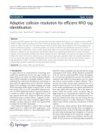
where un,k is the kth element of un . Now, instead of considering the system evolving only along time, we imagine a system progressing alternately along the path of time and the
¯
WMF observations yn,k . The concept is further illustrated
in Figure 1. To describe this new system, we must collapse
the time index n and the observation index k into one timeobservation index l, where l = (n − 1)K + k. This conversion
is reversible or, in other words, we can also calculate k and
n from l by k = mod(l, K) and n = (l − k)/K + 1, where
mod(k, K) is the k modulo K operation. In the following description of the TOSSM indexed by l, all k and n are assumed
to be obtained from the corresponding l. Now, we introduce
a K × K auxiliary matrix Bl = diag{bn,1 , . . . , bn,k , 0 . . . , 0}.
The state-space representation for the new time-observation
system indexed by l can be then constructed as

Qhl−1 + Gvl

hl = 
h l −1
¯
yl =

if k = 1,
if k = 1,

T
fk Bl Phl

¯
+ ul

(16)


Blind Multiuser Detection by Particle Filtering
TOSSM

133

TOSSM

TOSSM

TOSSM

¯
y1

¯
yK+1

¯
y(n−1)K+1

¯

ynK+1

¯
y2

¯
yK+2

¯
y(n−1)K+2

¯
ynK+2

DSSM y1 =

DSSM

y2 =

DSSM yn−1 =

DSSM

yn =

DSSM

¯
yK −1

¯
y2K −1

¯
ynk−1

¯
y(n+1)K −1

¯
yK

¯
y2K

¯
ynK

¯
y(n+1)K

TOSSM

TOSSM

TOSSM

TOSSM

Figure 1: Illustrative plot of the TOSSM.

and we call (16) the TOSSM. Note that (16) and (6) describe
the same system. There are, however, key differences between
the two models. Unlike (6), the state transitions of hl in the
TOSSM are time (or index) varying, that is, at different l,
different transition is applied. Specifically, when k = 1 or,
equivalently, n increases by 1, hl updates according to the
ARMA channel model, and otherwise when k = 1 and n remains unchanged from l − 1, hl is assumed to be static. Additionally, in the TOSSM, the number of the unknown user
bits changes with l and especially, only one new unknown
signal bn,k is included each time when l is incremented by
one. Therefore, if we assume perfect detection at l − 1, that is,
bn,1 , . . . , and bn,k−1 are known exactly, then there is only one
unknown user bit to be detected. Note that in the conventional DSSM (6), K unknown users bits need to be detected
altogether as the system evolves to time n. This is the key of
the model that leads to efficient particle filtering solutions.
We, however, want to stress that the decision on bn,k (except
k = K) is not finalized at l. Since the observations from yl+1
up to yl+r with r = K − k all contain information about bn,k ,
the final decision is reached only at l + r, or in general, when
k = K.
4.

OPTIMUM BAYESIAN BLIND DETECTION

In a Bayesian framework, the optimum decision on bN can
be obtained by the marginalized posterior mode (MPM) criterion, which is expressed as
bN,k

MPM

= sgn

¯
bn,k p bN | y1:NK

,

(17)

bN ∈{−1,1}K

¯
where p(bN | y1:NK ) is the posterior distribution that is essential for computing (17) and the subscript 1 : NK denotes a collection of the variable indexed from 1 to NK,
¯
¯
¯
e.g., y1:NK = { y1 , . . . , yNK }. Notice that the posterior dis¯
tribution p(bN | y1:NK ) is independent of b1:(N −1) , that is, the
bits transmitted prior to time n. Further, the marginalization
in (17) suggests that (bN,k )MPM is also independent of other
users’ bits transmitted at n. Therefore, the MPM solution is
immune to decision errors on b1:(N −1) and other users’ bits
transmitted at n.

¯
Now, to derive p(bn | y1:NK ), marginalization on p(b1:N |
¯
y1:NK ) over b1:(N −1) is needed, that is,
¯

p bN | y1:NK =

¯
p b1:N | y1:NK
b1:N −1

=

b1:N −1
b1:N

¯
p b1:N , y1:NK
.
¯
p b1:N , y1:NK

(18)

Considering the TOSSM (16), we found the joint distribution in (8), where the last equation was obtained by assuming the noninformative priors for bN,K , that is, p(bN,K =
1) = 0.5. Equation (8) indicates a recursive calculation of
¯
p(b1:N , y1:NK ) from l = 1 to NK through multiplying the
¯
¯
marginal likelihood p( yl |bn,1:k , b1:n−1 , y1:l ) at each recursion.
¯
¯
These likelihoods p( yl |bn,1:k , b1:n−1 , y1:l ) for l = 1, . . . , NK
are obtained by marginalizing the channel state vector hl

¯
¯
from p( yl , hl |bn,1:k , b1:n−1 , y1:l ), and we show in the appendix
that
¯
¯
p yl |bn,1:k , b1:n−1 , y1:l = N ml , cl

(19)

and the mean ml and variance cl can be calculated sequentially through the Kalman filter. This is equivalent to say
¯
that p( yl |bn,1:k , b1:n−1 ) can be calculated from a run of the
Kalman filter. Now, revisiting (18), we see that, to calculate
¯
¯
p(bN | y1:NK ), p( yl |bn,1:k , b1:n−1 ) must be evaluated for 2NK
combinations of b1:N , or 2NK Kalman filters are needed, each
of which corresponding to one possible combination. As a
result, totally 2NK Kalman filters are required for the MPM
solution. The expansion of the numbers of the Kalman filters with l presents a tree structure illustrated in Figure 2.
The MPM solution has thus a complexity exponentially increasing with both time n and the number of users K. This
is apparently a formidable task not possible for real applications. We, therefore, must resort to suboptimum solutions
with manageable complexity. One choice is particle filtering.
5.

A DECISION-DIRECTED APPROACH
TO BLIND MUD

A decision-directed approach to blind MUD was proposed in

[11] based on DSSM (6). We describe in the following a corresponding decision-directed approach on the TOSSM (16).


−1

bn,k =
−1

,k =

bn

bn,k =
−1

bn,k = −
1

bn,k =
−1

1

bn,k =
−1

b n,k =

1

=1

b n,k =

b n,k

1

=1

···

b n,k

b n,k =

1

=1

=

bn,k = 1

b n,k

b n,k

bn,k =
−1

EURASIP Journal on Wireless Communications and Networking

bn,k =
−1

134

=−

1

= −1

−1
1 =
,k −

bn

bn,k

bn,k

−1

−1

=−

bn,k

=1

=1

1

=1

=

−1

−1

b n,k−1

b n,k

b n,k−1

b n,k−1

1

l

l−1

···

1

−
,2
=

b1

−

1

2

=

1

b1

,1

,1
=

−

b1

1

1

,2
=

=

=

b1

2

2

b 1,

b 1,

1

3

1

Figure 2: The tree structure of the optimum solution. Each path in the tree represents a run of the Kalman filter.


Qh

l−1

Predictive step: hl = 
hl−1

QΞ

+ Gul

T
l−1 Q

Σl = 
Ξl−1

if k = 1,
if k = 1,

+ σ 2 GG

if k = 1,
if k = 1.

Detection step:
bn,k = sgn(zn,k );
¯
zn,k = ( yl −

k−1
∗
j =1 fk, j ai, j bi, j )ai,k ;

ai,k = ρk hl .
Update step:
Kl = Σl CH / cl with cl = Cl Σl CH + σ 2 ,
l
l
¯
hl = hl + Kl ( yl − Cl hl ),
Ξl = (I − Kl Cl )Σl ,
T
where Cl = fk Bl P and Bl = diag{[bn,1 , . . . , bn,k , 0 . . . , 0]}.

Algorithm 1: Decision-directed detector (DD).

One distinct feature of the decision-directed approach on the
TOSSM is that the decision on only one user’s bit is made at
each l. Specifically, let bn,k−1 and hl−1 represent the decisions
on bn,k−1 and hl−1 at l − 1, then the decision-directed approach at l can be summarized in Algorithm 1. Clearly, the
above decision-directed algorithm is equivalent to one run
of the Kalman filter, and therefore it is a lot simpler than
the optimum MPM solution. Nevertheless, the user bit is determined based on the prediction of the channel states and
the decisions on previous users’ bits, and thus it is not optimum. Compared with the algorithm based on DSSM (6),
at time k with k from 1 to K, the above algorithm makes

a decision on one user at a time and updates the channel
state vector hl whenever a decision is reached. The updated hl

will then influence the decision on bn,k+1 . Therefore, in both
a good and a bad way, decisions at early stages (smaller k)
would have more impact on decisions at later stages (larger
k) than those made by the algorithm on DSSM. If detection error exists in early stages, they will be propagated into
later stages. It is therefore beneficial to rank the users according to the estimated SNR. The performance of the decisiondirected algorithm is, however, ultimately limited by error
propagation.
6.

PARTICLE FILTERING DETECTOR
FOR BLIND MUD

Particle filtering belongs to the family of Monte Carlo sampling which aims at using samples to approximate posterior
distribution. However, particle filtering distinguishes itself by
employing a sequential importance sampling scheme, and
in particular, it is designed for nonlinear and non-Gaussian
systems described through state-space modeling such as the
problem concerned.
In the context of the proposed problem, when yN , or
¯
equivalently yN , is observed at time N, the objective of particle filtering is to draw, say, J weighted random samples
( j)
( j) J
( j)
¯
{b1:N , wNK } j =1 from p(b1:N | y1:nK ), where wNK is the weight
( j)
¯
of the jth sample b1:N . With the samples, p(bN | y1:NK ) can be
approximated by
J

¯
p b1:N | y1:nK ≈
j =1

( j)

wNK

NK
l =1

( j)

δ bn,k − bn,k ,

(20)


Blind Multiuser Detection by Particle Filtering

135

where δ(·) is the Dirac delta function, and hence the MPM
solution of b by a simple weighted summation is
J

bN,k

MPM

≈ sgn
j =1

( j)

( j)

(21)

wNK bN,k

for k = 1, . . . , K. By the law of large numbers, the approximation will converge to the true MPM solution with the increase
of the number of samples J. If these samples are taken directly
from the posterior distribution, then all the samples have
¯
equal weights. However, direct sampling from p(b1:N | y1:NK )
is prohibited since all possible combinations of b1:N must
¯
be evaluated on p(b1:N | y1:NK ), which again requires 2NK
Kalman filters. To circumvent the difficulty, importance sampling is performed where samples are taken from a proposal
¯
importance function π(b1:KN | y1:KN ) and weighted according
to
( j)

( j)

wKN =

¯
p b1:KN | y1:KN

∀ j.

( j)

¯
π b1:KN | y1:KN

(22)

¯
Notice that π(b1:KN | y1:KN ) is a very high-dimensional distribution and it is burdensome to sample the variables and
calculate the weights altogether. Fortunately, the TOSSM allows a Markovian factorization on the posterior distribution
as
¯
¯
¯
p b1:N , y1:NK ∝ p yNK |b1:N , y1:NK −1 p bN,K
¯
× p bN,1:K −1 , b1:N −1 | y1:NK −1
¯
¯
= p yNK |b1:N , y1:NK −1

(23)

¯
× p bN,1:K −1 , b1:N −1 | y1:NK −1 .

Then, if we choose the importance distribution as
¯
¯
π b1:N |y1:NK = p bN,k |bN,1:K −1 , b1:N −1 , y1:NK
¯
× π bN,1:K −1 , b1:N −1 | y1:NK −1 ,

(24)

the weight can be calculated by
( j)

( j)

wKN =

( j)

p
π

( j)
( j)
¯
bN,1:K −1 , b1:N −1 | y1:NK −1
( j)
( j)
¯
bN,1:K −1 , b1:N −1 | y1:NK −1
( j)

=

( j)

¯
¯
p yNK |b1:N , y1:NK −1 p bN,K
p

( j)
( j)
¯
bN,K |bN,1:K −1 , b1:N −1 , y1:NK
( j)

( j)

wKN −1

( j)

( j)

¯
¯
∝ p yNK |bN,1:K −1 , b1:N −1 , y1:NK −1 wKN −1
( j)

=

( j)

¯
¯
p yNK |b1:N , y1:NK −1 wKN −1
bN,K
( j)

( j)

( j)

( j)

( j)

= Nc mNK (i), cNK (i)
( j)

(26)
( j)

for i = 1, 2 where ml (i) and cl (i) are calculated the same
way as shown in the appendix but for a set of b1:NK given in
(26). We can therefore obtain samples and weights using a
recursive algorithm. To put the idea in concrete procedure,
we assume that at l − 1, we have obtained from a previous
( j)
recursion the trajectories (samples) {b0:l−1 }Jj =1 appropriately

( j)

weighted with the weights {wl−1 }Jj =1 . Using the recent ob¯
servations yl , we update the trajectories and weights as in
Algorithm 2. This process of recursively obtaining particles
( j)
is called particle filtering. After each recursion, the mean ηl
( j)
and covariance vectors Ξl are passed on to the next recursion. From (21), we also see that to calculate all the elements
( j)
of {bN }MPM , wNK is required. Therefore the decision on all
the elements can only be made after recursion l = KN and
the particles for bN,k for k = 1, 2, . . . , K − 1 must be stored.
In the above derivation of particle filtering, the adopted
importance function is known as optimum in the sense that
minimizes the variance of the weights. The above particle filtering procedure suffers from particle impoverishment, that
is, after several recursions, some weights of the samples become negligible and stop contributing to the overall evaluation. To prevent it, we insert a residue resampling step [15]
after every fixed recursion. Particularly, during the resam( j)
pling at recursion l, the particles for bn,1:k , the mean vectors,
and covariance matrices must be treated as a set in the resampling process.
7.

( j)

¯
p bN,K |bN,1:K −1 , b1:N −1 , y1:NK
×

( j)

¯
¯
λNK (i) = p yNK |bN,K = 2 ∗ i − 3, bN,1:K , b1:N , y1:NK −1

( j)

¯
¯
p yNK |b1:N , y1:NK −1 p bN,K
( j)

( j)

where µKN −1 is the weight update factor. Examining (24) and
( j)
(25), we find that given wKN −1 and p(bN,1:K −1 , b1:N −1 |
¯
y1:NK −1 ), the importance function (24) and the
( j)
¯
weights (25) are known exactly as long as p( yNK |b1:N ,
¯
y1:NK −1 ) can be derived. In fact, we have indicated in
¯
¯
Section 4 that p( yNK |b1:N , y1:NK −1 ) can be calculated
through the Kalman filter as

= µKN −1 wKN −1 ,

(25)

STOCHASTIC M-DETECTOR FOR BLIND MUD

Recently, a every efficient particle filtering algorithm called
stochastic M-algorithm (SMA) was proposed in [19] for
problems with discrete unknowns. SMA can provide similar performance as generic particle filtering but with much
reduced complexity. SMA can be considered as a particle filtering algorithm with the discrete delta functions as importance functions. In addition, each trajectory produces two
samples (−1 and 1) for the binary case rather than one sample as in the generic PF. A key feature with SMA is that no
two trajectories are identical, which is however rarely true
with the generic PF. As a result, the SMA can provide more
sample diversities with less trajectories than the generic PF.
Nonetheless, notice that the number of trajectories doubles
after each sampling and therefore a selection step is required


136

EURASIP Journal on Wireless Communications and Networking
For j = 1 to J, do as follows.

Trajectory expansion
(1) For j = 1 to J,
(i) perform the predictive step in the PFD Algorithm;
(ii) perform (2)(a) in Algorithm PFD;

(1) Predictive step:
Calculate

Qη( j) if k = 1,

 l−1
( j)
µl =  ( j)
η
if k = 1,
l−1
and 
QΞ j Q + σ 2 GG

l−1
( j)
Σl =  ( j)
Ξ
l−1
(2) Sampling step.

(2 j −1)

(iii) set bl
= 1 and calculate the weight by
(2 j −1)
( j)
( j)
¯
wl
= λl (1)wl−1 ;
(2 j)
(iv) set bl = −1 and calculate the weight by
(2 j −1)
( j)

( j)
¯
wl
= λl (−1)wl−1 ;
(2 j −1)
(v) form 2J new trajectories by setting bl
=
(2 j −1) ( j)
(2 j)
(2 j) ( j)
{bl
, b0:l } and bl = {bl , b0:l }.

if k = 1,
if k = 1.

(a) For i = 1 and −1, calculate
(i)

( j)

( j)

cl (i)

( j)

¯
(2) Normalize the weights wk to obtain wk .

( j)
ml (i)

( j)
( j)
= cl (i)µl and
j ( j) H
= cl (i)Σl cl (i) + σ 2 ,

(3) Trajectory selection: select J trajectories from 2M
trajectories using the optimal resampling algorithm.

( j)
( j)
T ( j)
where cl = fk Bl (i)P, Bl (i) =
( j)
( j)
diag{bn,1 , . . . , bn,k−1 , i, 0, . . . , 0};
( j)
( j)
( j)
(ii) λl (i) = Nc (ml (i), cl (i)).

(4) Updating step: for j = 1 to J;
perform the updating step in the PFD Algorithm.
Algorithm 3: Stochastic M detector (SMD).

(b) Sample m ∈ {−1, 1} with probability
( j)

proportional to λl (i) ∀i.
( j)

(c) Set bl = m.
( j)

(d) Calculate µl =
unnormalized

i∈{−1,1}
( j)
¯
weight wl

( j)

λl (i) and the
( j)

( j)

= µl wl−1 .

(3) Updating step. Calculate
( j)

( j)

( j)

( j)

j

(i) Kl = Σl c( j) (m)H /cl (m);
l
( j)

( j)

¯
(ii) ηl = µl + Kl ( yl − cl (m)µl );
( j)
Ξl

( j) ( j)
( j)
(iii)
= (I − Kl cl (m))Σl .
( j)
( j) ( j)
Form the new trajectories b0:l = {bl , b0:l−1 } ∀ j.
( j)
( j)
( j)
¯
¯
Normalize the weight as wl = wl / Jj =1 wl .

Algorithm 2: Particle filtering detector (PFD).

to avoid the exponential increase of trajectories. Here, we use
the optimal resampling algorithm [20] since it is a samplingwithout-replacement algorithm and does not produce replicates of the same trajectories, the feature that is required by
SMA. The SMA for the problem concerned at the lth recursion is outlined as in Algorithm 3.
The structure of the SMA resembles the popular Malgorithm. However, since the SMA is still a PF algorithm,
it can provide probability information about the unknowns
and thus can be applied to iterative MUD of a coded system.
7.1. Discussion on the MPM, decision-directed,
and particle filtering solutions
Comparing the PFD and the SMD with the decision-directed
algorithm, we see that the processes along each trajectory is
almost as identical as a decision-directed algorithm except
that a sampling step is used in the place of the detection step,
and they all resemble one run of Kalman filter which corresponds to a path in the tree of Figure 2. There are two paths
going out at every note in the tree, and in selecting a path,

the decision-directed algorithm uses a deterministic approach, while PFD and SMD adopt a soft measure which is
based on probability. What is more, each trajectory is also associated with a weight which indicates the significance of the
trajectory in final decision. Although trajectories with small
weight do not seem to contribute much to current decision
making at the present stage, they, however, might flourish in
later recursions and carry significant weights in decision. The
soft measure can apparently prevent current decision errors
from greatly influencing the future decision, a key advantage
over the decision-directed approach.
Comparing the PFD and the SMD with the optimum
MPM solution, PFD, especially the SMD, has clear edge in
complexity since it only maintains J trajectories or equivalently J Kalman filter at all times, but the required Kalman
filter for the MPM grows exponentially with time. Further,

the PFD and the SMD achieve every effective and efficient
approximation to the true posterior distribution and therefore provide decision performance closer to optimum. Since
the two detectors produce soft (probabilistic) results, they are
readily applied in turbo MUD.
8.

SIMULATION RESULTS

In this section, the bit error rate (BER) performance of the
proposed PFDs and SMDs are studied through experiments.
In all the experiments, the transmitted signal was differential
BPSK modulated. The number of users was 15. For the PFDs,
151 trajectories were maintained, whereas 4 and 32 trajectories were tested for SMDs. Further, an AR model was adopted
for the fading process, which was normalized to have a unit
power, and thus the signal-to-noise ratio (SNR) was obtained
by 10 log(1/σ 2 ).
In Figure 3, we provide the BER versus SNR for the different algorithms on a scenario of Ωd = 0.03. The genieaided detector is included as a lower bound. We notice that
the PFDs and SMDs with 32 trajectories are of the same


Blind Multiuser Detection by Particle Filtering

137

10−2

BER

10−1

10−1

BER

100

10−2

10−3

10−4
10

10−4

15

20

25

30

35

40

45

SNR

SM detector, 4 trajectories
SM detector, 32 trajectories

Figure 3: BERs versus SNR performance for various detectors. Ω =
0.03.

100

BER

10−1

10−2

10−3

15

20

25

30

35

40

45

SNR
Decision-directed detector
Particle filtering detector
Genie

10−5
10

15

20

25

30

35

40

45

SNR

Decision-directed detector
Particle filtering detector
Genie

10−4
10

10−3

SM detector, 4 trajectories
SM detector, 32 trajectories

Figure 4: BERs versus SNR performance for various detectors. Ω =
0.05.

order of magnitude as that of the genie-aided detector at
low SNR (less than 30 dB). On the other hand, the results obtained by the SMDs with 4 and 32 trajectories are
very close, especially after 20 dB, and comparable to that of
the PFD. The SMD with 4 trajectories is obviously more
favorable since it requires only about 1/35 of complexity
of the PFD. As a final note, the PFD and SMDs achieve
about 7 dB gain over the decision-directed detectors at 10−3

Decision-directed detector
Particle filtering detector
Genie

SM detector, 4 trajectories
SM detector, 32 trajectories

Figure 5: BERs versus SNR performance for various detectors for
users with different power. Ω = 0.03.

BER. In Figure 4, we provide the BER versus SNR performance for a higher Doppler frequency of Ωd = 0.05. Similar observations can be drawn as for the previous case even
though the overall performance of the detectors is worse,
which is reasonable considering that the channels are fading

faster.
In Figure 5, we provide the BER versus SNR of the first
user for the different algorithms on a scenario of Ωd =
0.03. In addition, the users have different power. The difference between the power of the first user and that of the
last user is 10 dB and the other users’ powers are equally
spaced in between. The genie-aided detector is also included
as a lower bound. In this case, the PFDs and SMDs with 32
trajectories are approximately of the same order of magnitude as that of the genie-aided detector at SNRs of the first
user less than 30 dB. As in the case of equal power, the results obtained by the SMDs with 4 and 32 trajectories are
very close, especially after 30 dB, and comparable to that of
the PFD. Again, the SMD with 4 trajectories is obviously
more favorable since it requires only about 1/35 of complexity of the PFD. In this experiment, the performance of the
decision-directed detector is much worse compared to the
performance of the PDF and SMDs. For example, the latter achieves about 11 dB gain over the former at 10−2 BER.
In Figure 6, we provide the BER versus SNR performance
for a Doppler frequency of Ωd = 0.05. Since the channels
considered are fading faster, the performance of the detectors is worse. However, in general, similar observations to
the tested detectors can be drawn. It is important to outline
that the performance of the decision-directed detector gets
worse in this case, for example, the PFD and SMDs achieve
about 20 dB gain over the decision-directed detectors at 10−2
BER.


138

EURASIP Journal on Wireless Communications and Networking
T
where Cl = fk Bl P. The second distribution p(hl |bn,1:k−1 ,
¯

b1:n−1 , y1:l−1 ) is the predictive density which can be obtained
from the predictive step of the Kalman filter [21, 22], that is,

10−1

10−2

BER

¯
p hl |bn,1:k−1 , b1:n−1 , y1:l−1 = N µl , Σl ,
10−3

(A.3)

where

Qη

l −1

µl = 
η l −1

10−4

if k = 1,
if k = 1,

(A.4)

and
10−5
10

15

20

25

30

35

40


QΞl−1 Q + σ 2 GG
Σl = 
Ξ

45

SNR
Decision-directed detector
Particle filter detector
Genie

l −1

SM detector, 4 trajectories
SM detector, 32 trajectories

Figure 6: BERs versus SNR performance for various detectors for
users with different power. Ω = 0.05.

if k = 1,
if k = 1.

(A.5)

In (A.4) and (A.5), ηl−1 and Ξl−1 are computed from the
update steps of the Kalman filter expressed in terms of l as
¯
ηl = µl + Kl yl − ml ,

(A.6)

Ξl = I − Kl Cl Σl ,

(A.7)

and
9.

CONCLUSION

In this paper, we proposed to solve blind MUD over flat fast
fading channels. We constructed a novel time-observation

state-space model, based on which efficient particle filtering
and stochastic M detectors were proposed. Particularly, the
detectors based on the SMA demonstrated greater potential
than those using generic PF. The former can provide comparable performance as the latter but with much smaller complexity.

where ml = Cl µl and Kl = Σl CH /cl with cl = Cl Σl CH + σ 2 .
l
l
Now the integration in (A.1) is readily derived as
¯
¯
p yl |bn,1:k , b1:n−1 , y1:l = N ml , cl .

(A.8)

ACKNOWLEDGMENTS

APPENDIX
¯
¯
DERIVATION OF THE LIKELIHOOD p( yl |bn,1:k , b1:n−1 , y1:l )
¯
¯
The likelihood p( yl |bn,1:k , b1:n−1 , y1:l ) can be obtained as
¯
¯
p yl |bn,1:k , b1:n−1 , y1:l−1
=

¯

¯
p yl , hl |bn,1:k , b1:n−1 , y1:l dht

=

REFERENCES

¯
¯
p yl |hl , bn,1:k p hl |bn,1:k−1 , b1:n−1 , y1:l−1 dhl ,

(A.1)

where the last equality is arrived by the fact that, given hl ,
¯
and bn,1:k , yl is independent of other variables, and hl is independent of bn,k . In (A.1), two distributions are involved in
the integral. The first distribution is the likelihood defined by
the observation equation which is
¯
p yl |hl , bn,1:k = N Cl hl , σ 2 ,

This work was supported by the National Science Foundation under Awards no. CCR-9903120 and no. CCR-0082607
and partially supported by the “Ministerio de Ciencia y Tecnolog´a,” Spain, under Project TIC 2001-2902.
ı

(A.2)

´
[1] S. Verdu, Multiuser Detection, Cambridge University Press,
New York, NY, USA, 1998.

[2] A. Russ and M. K. Varanasi, “Noncoherent multiuser detection for nonlinear modulation over the Rayleigh-fading channel,” IEEE Trans. Inform. Theory, vol. 47, no. 1, pp. 295–307,
2001.
[3] H.-Y. Wu and A. Duel-Hallen, “On the performance of coherent and noncoherent multiuser detectors for mobile radio CDMA channels,” in Proc. 5th IEEE International Conference on Universal Personal Communications, vol. 1, pp. 76–80,
Cambridge, Mass, USA, September–October 1996.
[4] M. Honig, U. Madhow, and S. Verdu, “Blind adaptive multiuser detection,” IEEE Trans. Inform. Theory, vol. 41, no. 4,
pp. 944–960, 1995.


Blind Multiuser Detection by Particle Filtering
[5] R. A. Iltis, “Exact and approximate maximum-likelihood parameter estimation for quasi-synchronous CDMA signals,”
IEEE Trans. Commun., vol. 48, no. 7, pp. 1208–1216, 2000.
[6] X. Wang and H. V. Poor, “Blind multiuser detection: a subspace approach,” IEEE Trans. Inform. Theory, vol. 44, no. 2,
pp. 677–690, 1998.
[7] U. Fawer and B. Aazhang, “A multiuser receiver for code division multiple access communications over multipath channels,” IEEE Trans. Commun., vol. 43, no. 234, pp. 1556–1565,
1995.
[8] K. Yen and L. Hanzo, “Genetic algorithm assisted joint multiuser symbol detection and fading channel estimation for
synchronous CDMA systems,” IEEE J. Select. Areas Commun.,
vol. 19, no. 6, pp. 985–998, 2001.
[9] T. J. Lim, L. K. Rasmussen, and H. Sugimoto, “An asynchronous multiuser CDMA detector based on the Kalman filter,” IEEE J. Select. Areas Commun., vol. 16, no. 9, pp. 1711–
1722, 1998.
[10] T. J. Lim and Y. Ma, “The Kalman filter as the optimal linear minimum mean-squared error multiuser CDMA detector,” IEEE Trans. Inform. Theory, vol. 46, no. 7, pp. 2561–2566,
2000.
[11] P. H.-Y. Wu and A. Duel-Hallen, “Multiuser detectors with
disjoint Kalman channel estimators for synchronous CDMA
mobile radio channels,” IEEE Trans. Commun., vol. 48, no. 5,
pp. 752–756, 2000.
[12] S. Vasudevan and M. K. Varanasi, “Achieving near-optimum
asymptotic efficiency and fading resistance over the timevarying Rayleigh-faded CDMA channel,” IEEE Trans. Commun., vol. 44, no. 9, pp. 1130–1143, 1996.
[13] K. J. Kim and R. A. Iltis, “Joint detection and channel estimation algorithms for QS-CDMA signals over time-varying
channels,” IEEE Trans. Commun., vol. 50, no. 5, pp. 845–855,

2002.
[14] B. Flanagan, C. Suprin, S. Kumaresan, and J. Dunyak, “Performance of a joint Kalman demodulator for multiuser detection,” in Proc. 56th IEEE Vehicular Technology Conference
(VTC ’02), vol. 3, pp. 1525–1529, Vancouver, Canada, 2002.
[15] R. Chen, X. Wang, and J. S. Liu, “Adaptive joint detection
and decoding in flat-fading channels via mixture Kalman filtering,” IEEE Trans. Inform. Theory, vol. 46, no. 6, pp. 2079–
2094, 2000.
[16] J. Zhang and P. M. Djuri´ , “Joint estimation and decoding
c
of space-time trellis codes,” EURASIP J. Appl. Signal Process.,
vol. 2002, no. 3, pp. 305–315, 2002.
[17] E. Punskaya, C. Andrieu, A. Doucet, and W. J. Fitzgerald,
“Particle filtering for multiuser detection in fading CDMA
channels,” in Proc. 11th IEEE Signal Processing Workshop
on Statistical Signal Processing, pp. 38–41, Singapore, August
2001.
[18] Y. Huang and P. M. Djuri´ , “A blind particle filtering detector
c
of signals transmitted over flat fading channels ,” IEEE Trans.
Signal Processing, vol. 52, no. 7, pp. 1891–1900, 2004.
[19] Y. Huang, J. Zhang, and P. M. Djuri´ , “Bayesian detection for
c
BLAST,” IEEE Transactions on Signal Processing, vol. 53, no. 3,
pp. 1086–1096, March 2005.
[20] P. Fearnhead, Sequential Monte Carlo method in filter theory,
Ph.D. thesis, Oxford University, Oxford, UK, 1998, available
from />[21] M. H. Hayes, Statistical Digital Signal Processing and Modeling,
John Wiley & Sons, New York, 1996.
[22] S. Haykin, Adaptive Filter Theory, Prentice Hall, Upper Saddle
River, NJ, USA, 4th edition, 2002.

139
Yufei Huang received the B.S. degree in applied electronics from Northwestern Polytechnical University, Xi’an, China, in 1995,
and the M.S. and Ph.D. degrees in electrical engineering from the State University of
New York at Stony Brook (SUNYSB), Stony
Brook, NY, in 1997 and 2001, respectively.
He is now an Assistant Professor in the
Department of Electrical Engineering, The
University of Texas at San Antonio. From
2001 to 2002, he worked as a Postdoctoral Researcher in the Department of Electrical and Computer Engineering, SUNYSB. His
current research interests are in Bayesian inference, Monte Carlo
methods, signal processing for communications, and bioinformatics.
Jianqiu (Michelle) Zhang received her B.S.
and M.S. degrees in electrical engineering
in 1992 and 1995, respectively, from Zhejiang University, Hangzhou University, and
Zhongshan University, Guangzhou, China.
From 1995 to 1997, she worked as a Software Engineer in R&D, Guangdong Nortel, China. She received her Ph.D. degree in
electrical engineering from the State University of New York at Stony Brook in 2002.
Currently, she is an Assistant Professor in the Department of Electrical and Computer Engineering at the University of New Hampshire. Her general research interest lies in the fields of wireless communications, information theory, and statistical methods in signal
processing. She had been working on topics including CDMA multiuser detection, turbo-coding, particle filtering, space-time coding, and channel capacity.
Isabel Tienda Luna was born in Dona
´
Menc´a, Cordoba, Spain, on October 5th
ı
1978. She received her B.S. and M.S. degrees
from the University of Granada, Spain, in
1999 and 2001, respectively. Now she is a
predoctoral researcher within the Systems,
Signals and Waves Research Group, Department of Applied Physics, the University of Granada. Her predoctoral research is
´
founded by the “Ministerio de Educaciøn y

Ciencia” of Spain. Her research interests are in the areas of digital
communications and signal processing including particle filtering
applications, channel estimation, and multiuser detection.
Petar M. Djuri´ received his B.S. and M.S.
c
degrees in electrical engineering from the
University of Belgrade, in 1981 and 1986,
respectively, and his Ph.D. degree in electrical engineering from the University of
Rhode Island in 1990. From 1981 to 1986 he
was a Research Associate with the Institute
of Nuclear Sciences, Vinca, Belgrade. Since
1990 he has been with Stony Brook University, where he is a Professor in the Department of Electrical and Computer Engineering. He works in the
area of statistical signal processing, and his primary interests are
in the theory of modeling, detection, estimation, and time series
analysis and its application to a wide variety of disciplines including wireless communications and biomedicine. Professor Djuri´
c


140
has served on numerous technical committees for the IEEE and
SPIE and has been invited to lecture at universities in the United
States and overseas. He is the Area Editor of special issues of the
Signal Processing Magazine and Associate Editor of the IEEE Transactions on Signal Processing. He is also Chair of the IEEE Signal
Processing Society Committee on Signal Processing—Theory and
Methods and is on the Editorial Board of Digital Signal Processing, the EURASIP Journal on Applied Signal Processing, and the
EURASIP Journal on Wireless Communications and Networking.
Professor Djuri´ is a Member of the American Statistical Associac
tion and the International Society for Bayesian Analysis.
Diego Pablo Ruiz Padillo was born in
´

Cabra, Cordoba, Spain, on July 17th 1968.
He received his B.S. and M.S. degrees in
electronic physics from the University of
Granada, in 1991 and 1993, respectively,
and his Ph.D. degree with honors in 1995.
He was a granted national researcher from
the “Ministerio de Ciencia y Tecnolog´a”
ı
of Spain, and an Assistant Professor in the
Universities of Malaga and Granada from
1991 to 1998. Now Dr. Diego P. Ruiz is an Associate Professor
within the Systems, Signals and Waves Research Group of the Department of Applied Physics in the University of Granada, Spain.
His research interests include statistical signal processing and its applications to wireless communications, blind channel identification
and equalization, adaptive algorithms, higher-order statistics, and
radar signal processing applied to transient electromagnetic problems.

EURASIP Journal on Wireless Communications and Networking