LYAPUNOV FUNCTIONALS CONSTRUCTION FOR STOCHASTIC DIFFERENCE SECOND-KIND VOLTERRA EQUATIONS WITH doc

LYAPUNOV FUNCTIONALS CONSTRUCTION
FOR STOCHASTIC DIFFERENCE SECOND-KIND
VOLTERRA EQUATIONS WITH CONTINUOUS TIME
LEONID SHAIKHET
Received 4 August 2003
The general method of Lyapunov functionals construction which was developed during
the last decade for stability investigation of stochastic differential equations with afteref-
fect and stochastic difference equations is considered. It is show n that after some mod-
ification of the basic Lyapunov-type theorem, this method can be successfully used also
for stochastic difference Volterra equations with continuous time usable in mathematical
models. The theoretical results are illustrated by numerical calculations.
1. Stability theorem
Construction of Lyapunov functionals is usually used for investigation of stability of
hereditary systems which are described by functional differential equations or Volterra
equations and have numerous applications [3, 4, 8, 21]. The general method of Lyapunov
functionals construction for stability investigation of hereditary systems was proposed
and developed (see [2, 5, 6, 7, 9, 10, 11, 12, 13, 17, 18, 19]) for both stochastic differential
equations with aftereffect and stochastic difference equations. Here it is shown that after
some modification of the basic Lyapunov-type stability theorem, this method can also be
used for stochastic difference Volterra equations with continuous time, which are popular
enough in researches [1, 14, 15, 16, 20].
Let
{Ω,F,P} be a probability space, {F
t
, t ≥ t
0
} a nondecreasing family of sub-σ-
algebras of F, that is, F
t
1
⊂ F

t
2
for t
1
<t
2
,andH aspaceofF
t
-measurable functions
x(t) ∈ R
n
, t ≥ t
0
,withnorms
x
2
= sup
t≥t
0
E


x(t)


2
, x
2
1
= sup

t∈[t
0
,t
0
+h
0
]
E


x(t)


2
. (1.1)
Consider the stochastic difference equation
x

t + h
0

=
η

t + h
0

+ F

t,x(t),x


t − h
1

,x

t − h
2

,

, t>t
0
− h
0
, (1.2)
Copyright © 2004 Hindawi Publishing Corporation
Advances in Difference Equations 2004:1 (2004) 67–91
2000 Mathematics Subject Classification: 39A11, 37H10
URL: />68 Difference Volterra equations with continuous time
with the initial condition
x(θ) = φ(θ), θ ∈ Θ =

t
0
− h
0
− max
j≥1
h

j
,t
0

. (1.3)
Here, η ∈ H, h
0
,h
1
, are positive constants, and φ(θ), θ ∈ Θ,isanF
t
0
-measurable func-
tion such that
φ
2
0
= sup
θ∈Θ
E


φ(θ)


2
< ∞, (1.4)
the functional F ∈ R
n
satisfies the condition



F

t,x
0
,x
1
,x
2
,



2
≤
∞

j=0
a
j


x
j


2
, A =
∞


j=0
a
j
< ∞. (1.5)
Asolutionofproblem(1.2), (1.3)isanF
t
-measurable process x(t) = x(t;t
0
,φ), which
is equal to the initial function φ(t)from(1.3)fort ≤ t
0
and with probability 1 defined by
(1.2)fort>t
0
.
Definit ion 1.1. A function x(t)fromH is called
(i) uniformly mean square bounded if x
2
< ∞;
(ii) asymptotically mean square trivial if
lim
t→∞
E


x(t)


2

= 0; (1.6)
(iii) asymptotically mean square quasitrivial if, for each t ≥ t
0
,
lim
j→∞
E


x

t + jh
0



2
= 0; (1.7)
(iv) uniformly mean square summable if
sup
t≥t
0
∞

j=0
E


x


t + jh
0



2
< ∞; (1.8)
(v) mean square integrable if

∞
t
0
E


x(t)


2
dt < ∞. (1.9)
Remark 1.2. It is easy to see that if the function x(t) is uniformly mean square summable,
then it is uniformly mean square bounded and asymptotically mean square quasitrivial.
Remark 1.3. It is evident that condition (1.7)followsfrom(1.6), but the inverse statement
is not true. The corresponding function is considered in Example 5.1.
Together with (1.2) we will consider the auxiliary difference equation
x

t + h
0


= F

t,x(t),x

t − h
1

,x

t − h
2

,

, t>t
0
− h
0
, (1.10)
with initial condition (1.3) and the functional F, satisfying condition (1.5).
Leonid Shaikhet 69
Definit ion 1.4. The trivial solution of (1.10)iscalled
(i) mean square stable if, for any  > 0andt
0
≥ 0, there exists a δ = δ(,t
0
) > 0such
that x(t)
2
<  if φ

2
0
<δ;
(ii) asymptotically mean square stable if it is mean square stable and for each initial
function φ, condition (1.6)holds;
(iii) asymptotically mean square quasistable if it is mean square stable and for each
initial function φ and each t ∈ [t
0
,t
0
+ h
0
), condition (1.7)holds.
Theorem 1.5. Let the process η(t) in (1.2) satisfy the condition η
2
1
< ∞, and there exist a
nonnegative functional
V(t) = V

t,x(t),x

t − h
1

,x

t − h
2


,

, (1.11)
positive numbers c
1
, c
2
, and nonnegative function γ(t), such that
ˆ
γ = sup
s∈[t
0
,t
0
+h
0
)
∞

j=0
γ

s + jh
0

< ∞, (1.12)
EV(t) ≤ c
1
sup
s≤t

E|x( s)|
2
, t ∈

t
0
,t
0
+ h
0

, (1.13)
E∆V(t) ≤−c
2
E|x( t)|
2
+ γ(t), t ≥ t
0
, (1.14)
where
∆V(t) = V(t + h
0
) − V(t). (1.15)
Then the solution of (1.2), (1.3) is uniformly mean square summable.
Proof. Rewrite condition (1.14)intheform
E∆V

t + jh
0


≤−c
2
E


x

t + jh
0



2
+ γ

t + jh
0

, t ≥ t
0
, j = 0,1, (1.16)
Summing this inequality from j = 0to j = i,byvirtueof(1.15), we obtain
EV

t +(i +1)h
0

− EV(t) ≤−c
2
i


j=0
E


x

t + jh
0



2
+
i

j=0
γ

t + jh
0

. (1.17)
Therefore,
c
2
∞

j=0
E



x

t + jh
0



2
≤ EV(t)+
∞

j=0
γ

t + jh
0

, t ≥ t
0
. (1.18)
70 Difference Volterra equations with continuous time
We show that the right-hand side of inequality (1.18) is bounded. Really, using (1.14),
(1.15), for t ≥ t
0
,wehave
EV(t) ≤ EV

t − h

0

+ γ

t − h
0

≤ EV

t − 2h
0

+ γ

t − 2h
0

+ γ

t − h
0

≤···≤ EV

t − ih
0

+
i


j=1
γ

t − jh
0

≤···≤ EV(s)+
τ

j=1
γ

t − jh
0

,
(1.19)
where
s = t − τh
0
∈

t
0
,t
0
+ h
0

, τ =


t − t
0
h
0

, (1.20)
[t]istheintegerpartofanumbert.
Since t = s +τh
0
,then
∞

j=0
γ

t + jh
0

=
∞

j=0
γ

s +(τ + j)h
0

=
∞


j=τ
γ

s + jh
0

,
τ

j=1
γ

t − jh
0

=
τ

j=1
γ

s +(τ − j)h
0

=
τ−1

j=0
γ


s + jh
0

.
(1.21)
Therefore, using (1.12), we obtain
∞

j=0
γ

t + jh
0

+
τ

j=1
γ

t − jh
0

=
∞

j=0
γ


s + jh
0

≤
ˆ
γ. (1.22)
So, from (1.18), (1.19), and (1.22), it follows that
c
2
∞

j=0
E


x

t + jh
0



2
≤
ˆ
γ + EV(s), t ≥ t
0
, s = t −

t − t

0
h
0

, h
0
∈

t
0
,t
0
+ h
0

.
(1.23)
Using (1.13), we get
sup
s∈[t
0
,t
0
+h
0
)
EV(s) ≤ c
1
sup
t≤t

0
+h
0
E


x(t)


2
≤ c
1

φ
2
0
+ x
2
1

. (1.24)
Leonid Shaikhet 71
From (1.2), (1.3), and (1.5), for t ∈ [t
0
,t
0
+ h
0
], we obtain
E



x(t)


2
= E


η(t)+F

t − h
0
,x

t − h
0

,x

t − h
0
− h
1

,x

t − h
0
− h

2

,



2
≤ 2

E


η(t)


2
+ E


F

t − h
0
,x

t − h
0

,x


t − h
0
− h
1

,x

t − h
0
− h
2

,



2

≤ 2


E


η(t)


2
+ a
0

E


φ

t − h
0



2
+
∞

j=1
a
j
E


φ

t − h
0
− h
j



2



≤ 2

η
2
1
+ Aφ
2
0

.
(1.25)
Using (1.23), (1.24), and (1.25), we have
c
2
∞

j=0
E


x

t + jh
0



2

≤
ˆ
γ + c
1

(1 + 2A)φ
2
0
+2η
2
1

. (1.26)
From here and (1.8), it follows that the solution of (1.2), (1.3) is uniformly mean square
summable. The theorem is proven. 
Remark 1.6. Replace condition (1.12)inTheorem 1.5 by the condition

∞
t
0
γ(t)dt < ∞. (1.27)
Then the solution of (1.2) for each initial function (1.3) is mean square integrable. Really,
integrating (1.14)fromt
= t
0
to t = T,byvirtueof(1.15), we have

T
t
0

E

V

t + h
0

− V(t)

dt ≤−c
2

T
t
0
E


x(t)


2
dt +

T
t
0
γ(t)dt (1.28)
or


T+h
0
T
EV(t)dt −

t
0
+h
0
t
0
EV(t)dt ≤−c
2

T
t
0
E


x(t)


2
dt +

T
t
0
γ(t)dt. (1.29)

From here and (1.24), (1.25), it follows that
c
2

T
t
0
E


x(t)


2
dt ≤

t
0
+h
0
t
0
EV(t)dt +

T
t
0
γ(t)dt
≤ c
1

h
0

(1 + 2A)φ
2
0
+2η
2
1

+

∞
t
0
γ(t)dt < ∞,
(1.30)
and by T
→∞,weobtain(1.9).
Remark 1.7. Suppose that for (1.10) the conditions of Theorem 1.5 hold with γ(t) ≡ 0.
Then the trivial solution of (1.10) is asymptotically mean square quasistable. Really, in
the case γ(t) ≡ 0 from inequality (1.26)for(1.10)(η(t) ≡ 0), it follows that c
2
E|x(t)|
2
≤
c
1
(1 + 2A)φ
2

0
and condition (1.7) follows. It means that the trivial solution of (1.10)is
asymptotically mean square quasistable.
72 Difference Volterra equations with continuous time
From Theorem 1.5 and Remark 1.6, it follows that an investigation of the solution of
(1.2) can be reduce d to the construction of appropriate Lyapunov functionals. Below,
some formal procedure of Lyapunov functionals construction for (1.2)isdescribed.
Remark 1.8. Supposethatin(1.2) h
0
= h>0, h
j
= jh, j = 1,2, Putting t = t
0
+ sh,
y(s) = x(t
0
+ sh), and ξ(s) = η(t
0
+ sh), one can reduce (1.2)totheform
y(s +1)= ξ(s +1)+G

s, y(s), y(s − 1), y(s − 2),

, s>−1,
y(θ) = φ(θ), θ ≤ 0.
(1.31)
Below,theequationoftype(1.31) is considered.
2. Formal procedure of Lyapunov functionals construction
The proposed procedure of Lyapunov functionals construction consists of the following
four steps.

Step 1. Represent the functional F at the right-hand side of (1.2)intheform
F

t,x(t),x

t − h
1

,x

t − h
2

,

=
F
1
(t)+F
2
(t)+∆F
3
(t), (2.1)
where
F
1
(t) = F
1

t,x(t),x


t − h
1

, ,x

t − h
k

,
F
j
(t) = F
j

t,x(t),x

t − h
1

,x

t − h
2

,

, j = 2,3,
F
1

(t,0, ,0)≡ F
2
(t,0,0, ) ≡ F
3
(t,0,0, ) ≡ 0,
(2.2)
k ≥ 0isagiveninteger,∆F
3
(t) = F
3
(t + h
0
) − F
3
(t).
Step 2. Suppose that for the auxiliary equation
y

t + h
0

=
F
1

t, y(t), y

t − h
1


, , y

t − h
k

, t>t
0
− h
0
, (2.3)
there exists a Lyapunov functional
v(t) = v

t, y(t), y

t − h
1

, , y

t − h
k

, (2.4)
which satisfies the conditions of Theorem 1.5.
Step 3. Consider Lyapunov functional V (t)for(1.2)intheformV(t) = V
1
(t)+V
2
(t),

where the main component is
V
1
(t) = v

t,x(t) − F
3
(t),x

t − h
1

, ,x

t − h
k

. (2.5)
Calculate E∆V
1
(t) and, in a reasonable way, estimate it.
Step 4. In order to satisfy the conditions of Theorem 1.5, the additional component V
2
(t)
is chosen by some standard way.
Leonid Shaikhet 73
3. Linear Volterra equations with constant coefficients
We demonstrate the formal procedure of Lyapunov functionals construction described
above for stability investigation of the scalar equation
x(t +1)= η(t +1)+

[t]+r

j=0
a
j
x(t − j), t>−1,
x(s) = φ(s), s ∈

− (r +1),0

,
(3.1)
where r ≥ 0isagiveninteger,a
j
are known constants, and the process η(t)isuniformly
mean square summable.
3.1. The first way of Lyapunov functionals construct ion. Following the procedure,
represent (Step 1) equation (3.1)intheform(2.1)withF
3
(t) = 0,
F
1
(t) =
k

j=0
a
j
x(t − j), F
2

(t) =
[t]+r

j=k+1
a
j
x(t − j), k ≥ 0, (3.2)
and consider (Step 2) the auxiliary equation
y(t +1)=
k

j=0
a
j
y(t − j), t>−1, k ≥ 0,
y(s) =



φ(s), s ∈

− (r +1),0

,
0, s<−(r +1).
(3.3)
Take into consideration the vector Y(t) = (y(t − k), , y(t − 1), y(t))

and represent the
auxiliary equation (3.3)intheform

Y(t +1)= AY(t), A =









01 0··· 00
00 1··· 00
.
.
.
.
.
.
.
.
.
.
.
.
.
.
.
.
.
.

00 0
··· 01
a
k
a
k−1
a
k−2
··· a
1
a
0









. (3.4)
Consider the matrix equation
A

DA− D =−U, U =







0 ··· 00
.
.
.
.
.
.
.
.
.
.
.
.
0
··· 00
0 ··· 01






, (3.5)
and suppose that the solution D of this equation is a positive semidefinite symmetric ma-
trix of dimension k + 1 with the elements d
ij
such that the condition d
k+1,k+1

> 0holds.In
74 Difference Volterra equations with continuous time
this case the function v(t) = Y

(t)DY(t)isaLyapunovfunctionfor(3.4), that is, it sat-
isfies the conditions of Theorem 1.5, in particular, condition (1.14)withγ(t) = 0. Really,
using (3.4), we have
∆v(t) = Y

(t +1)DY(t +1)− Y

(t)Dy(t)
= Y

(t)[A

DA− D]Y(t) =−Y

(t)UY(t) =−y
2
(t).
(3.6)
Following Step 3 of the procedure, we w ill construct a Lyapunov functional V(t)for
(3.1)intheformV(t)
= V
1
(t)+V
2
(t), where
V

1
(t) = X

(t)DX(t), X(t) =

x(t − k), ,x(t − 1),x(t)


. (3.7)
Rewrite now (3.1) using representation (3.2)as
X(t +1)= AX(t)+B(t),
B(t) =

0, ,0,b(t)


, b(t) = η(t +1)+F
2
(t),
(3.8)
where the matrix A is defined by (3.4). Calculating ∆V
1
(t), by virtue of (3.8), we have
∆V
1
(t) = X

(t +1)DX(t +1)− X

(t)DX(t)

=

AX(t)+B(t)


D

AX(t)+B(t)

− X

(t)DX(t)
=−x
2
(t)+B

(t)DB(t)+2B

(t)DAX(t).
(3.9)
Put
α
l
=
∞

j=l


a

j


, l = 0, 1, (3.10)
Using (3.8), (3.2), (3.10), and µ>0, we obtain
EB

(t)DB(t)
= d
k+1,k+1
Eb
2
(t) = d
k+1,k+1
E

η(t +1)+F
2
(t)

2
≤ d
k+1,k+1

(1 + µ)E


η(t +1)



2
+

1+µ
−1

EF
2
2
(t)

=
d
k+1,k+1



(1 + µ)E


η(t +1)


2
+

1+µ
−1

E



[t]+r

j=k+1
a
j
x( t − j)


2



≤ d
k+1,k+1


(1 + µ)E


η(t +1)


2
+

1+µ
−1


α
k+1
[t]+r

j=k+1


a
j


Ex
2
(t − j)


.
(3.11)
Leonid Shaikhet 75
Since
DB(t) = b(t)










d
1,k+1
d
2,k+1
.
.
.
d
k,k+1
d
k+1,k+1









, AX(t) =













x(t − k +1)
x(t − k +2)
.
.
.
x(t)
k

m=0
a
m
x(t − m)












, (3.12)
then
EB


(t)DAX(t)
= Eb(t)


k

l=1
d
l,k+1
x(t − k + l)+d
k+1,k+1
k

m=0
a
m
x(t − m)


=
Eb(t)


k−1

m=0

a
m

d
k+1,k+1
+ d
k−m,k+1

x(t − m)+a
k
d
k+1,k+1
x( t − k)


=
d
k+1,k+1
k

m=0
Q
km
Eb(t)x(t − m),
(3.13)
where
Q
km
= a
m
+
d
k−m,k+1

d
k+1,k+1
, m = 0, ,k − 1, Q
kk
= a
k
. (3.14)
Note that
k

m=0
Q
km
Eb(t)x(t − m) =
k

m=0
Q
km
Eη(t +1)x(t − m)+EF
2
(t)
k

m=0
Q
km
x(t − m),
(3.15)
and for µ>0,

2


Eη(t +1)x(t − m)


≤ µEη
2
(t +1)+µ
−1
Ex
2
(t − m). (3.16)
Putting
β
k
=
k

m=0


Q
km


=


a

k


+
k−1

m=0





a
m
+
d
k−m,k+1
d
k+1,k+1





(3.17)
76 Difference Volterra equations with continuous time
and using (3.2), (3.10), and (3.17), we obtain
2EF
2
(t)

k

m=0
Q
km
x(t − m)
= 2
k

m=0
[t]+r

j=k+1
Q
km
a
j
Ex( t − m) x(t − j)
≤
k

m=0
[t]+r

j=k+1


Q
km





a
j



Ex
2
(t − m)+Ex
2
(t − j)

≤
k

m=0


Q
km




α
k+1
Ex
2

(t − m)+
[t]+r

j=k+1


a
j


Ex
2
(t − j)


=
α
k+1
k

m=0


Q
km


Ex
2
(t − m)+β

k
[t]+r

j=k+1


a
j


Ex
2
(t − j).
(3.18)
So,
2EB

(t)DAX(t) ≤ d
k+1,k+1


β
k
[t]+r

j=k+1


a
j



Ex
2
(t − j)+β
k
µEη
2
(t +1)
+

α
k+1
+ µ
−1

k

m=0


Q
km


Ex
2
(t − m)



.
(3.19)
From (3.9), (3.11), and (3.19), we have
E∆V
1
(t) ≤−Ex
2
(t)+d
k+1,k+1
×



1+µ
−1

α
k+1
+ β
k

[t]+r

j=k+1


a
j



Ex
2
(t − j)
+

1+µ

1+β
k

Eη
2
(t +1)+

α
k+1
+ µ
−1

k

m=0


Q
km


Ex
2

(t − m)


.
(3.20)
Put now
R
km
=




α
k+1
+ µ
−1



Q
km


,0≤ m ≤ k,

1+µ
−1

α

k+1
+ β
k



a
m


, m>k.
(3.21)
Then (3.20) takes the form
E∆V
1
(t) ≤−Ex
2
(t)+d
k+1,k+1



1+µ

1+β
k

Eη
2
(t +1)+

[t]+r

m=0
R
km
Ex
2
(t − m)


.
(3.22)
Leonid Shaikhet 77
Choose now (Step 4) the functional V
2
(t)intheform
V
2
(t) = d
k+1,k+1
[t]+r

m=1
q
m
x
2
(t − m), q
m
=

∞

j=m
R
kj
. (3.23)
Then
∆V
2
(t) = d
k+1,k+1


[t]+1+r

m=1
q
m
x
2
(t +1− m) −
[t]+r

m=1
q
m
x
2
(t − m)



=
d
k+1,k+1


[t]+r

m=0
q
m+1
x
2
(t − m) −
[t]+r

m=1
q
m
x
2
(t − m)


=
d
k+1,k+1


q

1
x
2
(t) −
[t]+r

m=1
R
km
x
2
(t − m)


.
(3.24)
From (3.22), (3.24), for the functional V(t) = V
1
(t)+V
2
(t), we have
E∆V(t) ≤−

1 − q
0
d
k+1,k+1

Ex
2

(t)+γ(t), (3.25)
where
γ(t) = d
k+1,k+1

1+µ

1+β
k

Eη
2
(t +1). (3.26)
Since the process η(t) is uniformly mean square summable, then the function γ(t) satisfies
condition (1.12). So, if
q
0
d
k+1,k+1
< 1, (3.27)
then the functional V(t) satisfies condition (1.14). It is easy to check that condition (1.13)
holds too. Really, using (3.7), (3.23) for the functional V(t)
= V
1
(t)+V
2
(t)andt ∈ [0,1),
we have
EV(t) ≤D
k


j=0
Ex
2
(t − j)+d
k+1,k+1
r

m=1
q
m
Ex
2
(t − m)
≤

(k +1)D + d
k+1,k+1
r

m=1
q
m

sup
s≤t
Ex
2
(s).
(3.28)

So, if condition (3.27) holds, then the solution of (3.1) is uniformly mean square sum-
mable.
78 Difference Volterra equations with continuous time
Using (3.23), (3.21), (3.17), and (3.10), transform q
0
in the following way:
q
0
=
∞

j=0
R
kj
=
k

j=0
R
kj
+
∞

j=k+1
R
kj
=

α
k+1

+ µ
−1

k

j=0


Q
kj


+

1+µ
−1

α
k+1
+ β
k

∞

j=k+1


a
j



=

α
k+1
+ µ
−1

β
k
+

1+µ
−1

α
k+1
+ β
k

α
k+1
= α
2
k+1
+2α
k+1
β
k
+ µ

−1

α
2
k+1
+ β
k

.
(3.29)
Thus, if
α
2
k+1
+2α
k+1
β
k
<d
−1
k+1,k+1
, (3.30)
then there exists a so big µ>0 that condition (3.27) holds and, therefore, the solution of
(3.1) is uniformly mean square summable.
Note that condition (3.30) can also be represented in the for m
α
k+1
<

β

2
k
+ d
−1
k+1,k+1
− β
k
. (3.31)
Remark 3.1. Suppose that in (3.1)
a
j
= 0, j>k. (3.32)
Then α
k+1
= 0. So, if condition (3.32) holds and the matrix equation (3.5) has a positive
semidefinite solution D with d
k+1,k+1
> 0, then the solution of (3.1)isuniformlymean
square summable.
3.2. The second way of Lyapunov functionals construction. We get another stability
condition. Equation (3.1)canberepresented(Step 1)intheform(2.1)withF
2
(t) = 0,
k = 0,
F
1
(t) = βx(t), β =
∞

j=0

a
j
, F
3
(t) =−
[t]+r

m=1
x(t − m)
∞

j=m
a
j
. (3.33)
Really, calculating ∆F
3
(t), we have
∆F
3
(t) =−
[t]+1+r

m=1
x(t +1− m)
∞

j=m
a
j

+
[t]+r

m=1
x(t − m)
∞

j=m
a
j
=−
[t]+r

m=0
x(t − m)
∞

j=m+1
a
j
+
[t]+r

m=1
x(t − m)
∞

j=m
a
j

=−x(t)
∞

j=1
a
j
+
[t]+r

m=1
x(t − m)a
m
.
(3.34)
Leonid Shaikhet 79
Thus,
x(t +1)= η(t +1)+βx(t)+∆F
3
(t). (3.35)
In this case the auxiliary equation (2.3)(Step 2)isy(t +1)= βy(t). The function
v(t) = y
2
(t) is a Lyapunov function for this equation if |β| < 1. We will construct the
Lyapunov functional V(t)(Step 3)for(3.1)intheformV(t) = V
1
(t)+V
2
(t), where
V
1

(t) = (x(t)− F
3
(t))
2
.CalculatingE∆V
1
(t), by virtue of representation (3.33), we have
E∆V
1
(t) = E


x(t +1)− F
3
(t +1)

2
−

x(t)− F
3
(t)

2

= E


η(t +1)+βx(t) − F
3

(t)

2
−

x(t)− F
3
(t)

2

=
E

η(t +1)+(β − 1)x(t)

η(t +1)+(β +1)x(t) − 2F
3
(t)

=

β
2
− 1

Ex
2
(t)+Eη
2

(t +1)+2βEη(t +1)x(t)
− 2Eη(t +1)F
3
(t) − 2(β − 1)Ex(t)F
3
(t).
(3.36)
Using µ>0, we obtain
2E


η(t +1)x(t)


≤ µEη
2
(t +1)+µ
−1
Ex
2
(t). (3.37)
Putting
B
m
=







∞

j=m
a
j






, α =
∞

m=1
B
m
(3.38)
and using (3.33), (3.10), we have
2E


η(t +1)F
3
(t)


≤ 2
[t]+r


m=1
B
m
E


η(t +1)x(t − m)


≤
[t]+r

m=1
B
m

µEη
2
(t +1)+µ
−1
Ex
2
(t − m)

≤ αµEη
2
(t +1)+µ
−1
[t]+r


m=1
B
m
Ex
2
(t − m),
2E


x(t)F
3
(t)


≤ 2
[t]+r

m=1
B
m
E


x(t)x(t − m)


≤
[t]+r


m=1
B
m

Ex
2
(t)+Ex
2
(t − m)

≤ αEx
2
(t)+
[t]+r

m=1
B
m
Ex
2
(t − m).
(3.39)
80 Difference Volterra equations with continuous time
As a result,
E∆V
1
(t) ≤

β
2

− 1+α|β − 1| + µ
−1
|β|

Ex
2
(t)+

1+µ

α + |β|

Eη
2
(t +1)
+

|β − 1| + µ
−1

[t]+r

m=1
B
m
Ex
2
(t − m).
(3.40)
Put now (Step 4)

V
2
(t) =
[t]+r

m=1
γ
m
x
2
(t − m), γ
m
=

|
β − 1| + µ
−1

∞

j=m
B
j
. (3.41)
Then, using (3.38), similar to (3.24), we have
∆V
2
(t) =

|β − 1| + µ

−1



αx
2
(t) −
[t]+r

m=1
B
m
x
2
(t − m)


. (3.42)
So, for the functional V(t) = V
1
(t)+V
2
(t), we obtain
E∆V(t) ≤

β
2
− 1+2α|β − 1| + µ
−1


α + |β|

Ex
2
(t)
+

1+µ

α + |β|

Eη
2
(t +1).
(3.43)
Thus, if
β
2
+2α|β − 1| < 1, (3.44)
then there exists a so big µ>0thatconditionβ
2
+2α|β − 1| + µ
−1
(α + |β|) < 1holdsalso,
and, therefore, the solution of (3.1) is uniformly mean square summable.
It is easy to see that condition (3.44) can be written also in the form
1+β>2α, |β| < 1. (3.45)
4. Part icular cases
Here, particular cases of condition (3.31)fordifferent k
≥ 0 are considered.

4.1. Case k = 0. Equation (3.5) gives the solution d
11
= (1 − a
2
0
)
−1
, which is a positive
one if |a
0
| < 1. From (3.17), it follows that β
0
=|a
0
|. Condition (3.31) takes the form
α
0
< 1. (4.1)
So, under condition (4.1), the solution of (3.1) is uniformly mean square summable.
4.2. Case k
= 1. The matrix equation (3.5) is equivalent to the system of equations
a
2
1
d
22
− d
11
= 0,


a
1
− 1

d
12
+ a
0
a
1
d
22
= 0,
d
11
+2a
0
d
12
+

a
2
0
− 1

d
22
=−1,
(4.2)

Leonid Shaikhet 81
with the solution
d
11
= a
2
1
d
22
, d
12
=
a
0
a
1
1 − a
1
d
22
,
d
22
=
1 − a
1

1+a
1




1 − a
1

2
− a
2
0

.
(4.3)
The matrix D is a positive semidefinite one with d
22
> 0 by conditions |a
1
| < 1, |a
0
| <
1 − a
1
. Using (3.17), (4.3), we have
β
1
=


a
1



+




a
0
+
d
12
d
22




=


a
1


+




a

0
+
a
0
a
1
1 − a
1




=


a
1


+


a
0


1 − a
1
,
d

−1
22
= 1 − a
2
1
− a
2
0
1+a
1
1 − a
1
.
(4.4)
Condition (3.31) takes the form
α
2
<

1 −


a
1




1 −



a
0


1 − a
1

. (4.5)
Under condition (4.5), the solution of (3.1) is uniformly mean square summable.
Note that condition (4.5) can also be written in the form
α
0
< 1+


a
0




a
1


− a
1
1 − a
1

. (4.6)
It is easy to see that condition (4.6)isnotworsethan(4.1). In particular, for a
1
≥ 0,
condition (4.6) coincides with (4.1).
4.3. Case k = 2. The matrix equation (3.5) is equivalent to the system of equations
a
2
2
d
33
− d
11
= 0,
a
2
d
13
+ a
1
a
2
d
33
− d
12
= 0,
a
2
d

23
+ a
0
a
2
d
33
− d
13
= 0,
d
11
+2a
1
d
13
+ a
2
1
d
33
− d
22
= 0,
d
12
+ a
0
d
13

+ a
0
a
1
d
33
+

a
1
− 1

d
23
= 0,
d
22
+2a
0
d
23
+

a
2
0
− 1

d
33

=−1,
(4.7)
82 Difference Volterra equations with continuous time
with the solution
d
11
= a
2
2
d
33
,
d
12
=
a
2

1 − a
1

a
1
+ a
0
a
2

1 − a
1

− a
2

a
0
+ a
2

d
33
,
d
13
=
a
2

a
0
+ a
1
a
2

1 − a
1
− a
2

a

0
+ a
2

d
33
,
d
22
=

a
2
1
+ a
2
2
+
2a
1
a
2

a
0
+ a
1
a
2


1 − a
1
− a
2

a
0
+ a
2


d
33
,
d
23
=

a
0
+ a
2

a
1
+ a
0
a
2


1 − a
1
− a
2

a
0
+ a
2

d
33
,
(4.8)
d
33
=

1 − a
2
0
− a
2
1
− a
2
2
− 2
a
1

a
2

a
0
+ a
1
a
2

+ a
0

a
0
+ a
2

a
1
+ a
0
a
2

1 − a
1
− a
2


a
0
+ a
2


−1
. (4.9)
Using (3.17), (4.7), and (4.8), we have
β
2
=


a
2


+




a
0
+
d
23
d
33





+




a
1
+
d
13
d
33




=


a
2


+



d
13


+


d
12




a
2


d
33
=


a
2


+


a

0
+ a
1
a
2


+



1 − a
1

a
1
+ a
0
a
2





1 − a
1
− a
2


a
0
+ a
2



.
(4.10)
If the matrix D with the elements defined by (4.8) is a positive semidefinite one with
d
33
> 0, then under the condition
α
3
<

β
2
2
+ d
−1
33
− β
2
, (4.11)
the solution of (3.1) is uniformly mean square summable.
5. Examples
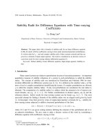
Example 5.1. Consider the difference equation
x(t +1)= η(t +1)+ax(t)+bx(t − 1), t>−1,

x(θ) = φ(θ), θ ∈ [−2,0].
(5.1)
From conditions (4.1)and(4.5)followtwosufficient conditions for uniformly mean
square summability of the solution of (5.1):
|a| + |b| < 1, (5.2)
|a| + b<1, |b| < 1. (5.3)
Condition (4.11)for(5.1) coincides with (5.3). Condition (3.45) takes the form
1+a + b>2|b|, |a + b| < 1. (5.4)
Leonid Shaikhet 83
−1
A
2
3
1
a
21
0
−1−2
B
1
b
Figure 5.1
On Figure 5.1 are shown the regions of uniformly mean square summability, obtained
for (5.1) by conditions (5.2) (the square number 1), (5.3) (the triangle number 2), and
(5.4)(thetrianglenumber3).
For numerical investigation of the solution of (5.1), we determine one of the possible
trajectories of the process η(t), t ≥ t
0
, in the following way. On the interval [t
0

+ nh
0
,t
0
+
(n +1)h
0
), n = 0,1, ,put
η(t) = 0 (5.5)
if
t ∈

t
0
+ nh
0
,t
0
+

n +1−
1
2
n

h
0

(5.6)
or

t ∈

t
0
+

n +1−
1
2
n+1

h
0
,t
0
+(n +1)h
0

, (5.7)
put
η(t)
= 2
n+2

t − t
0
h
0
− n − 1+
1

2
n

(5.8)
if
t
∈

t
0
+

n +1−
1
2
n

h
0
,t
0
+

n +1−
3
2
n+2

h
0


, (5.9)
and put
η(t) = 1 − 2
n+2

t − t
0
h
0
− n − 1+
3
2
n+2

(5.10)
84 Difference Volterra equations with continuous time
0
1234567
t
1
η
Figure 5.2
−210203040506070
t
−2
−1
1
2
x

Figure 5.3
if
t ∈

t
0
+

n +1−
3
2
n+2

h
0
,t
0
+

n +1−
1
2
n+1

h
0

. (5.11)
Thegraphofthefunctionη(t)fort
0

= 0, h
0
= 1 is shown on Figure 5.2.
The function η(t) constructed above satisfies the following conditions:
0 ≤ η(t) ≤ 1,
∞

j=0
η

t + jh
0

≤ 1,

∞
0
η(t)dt =
1
2
. (5.12)
It is easy to see also that for each fixed t ∈ [t
0
,t
0
+ h
0
), the sequence η
j
= η(t + jh

0
)has
only one nonzero member, and therefore lim
j→∞
η(t + jh
0
) = 0. On the other hand, for
every T>0, there exists a so large number n that
t
1
= t
0
+

n +1−
3
2
n+2

h
0
>T, η

t
1

= 1. (5.13)
Leonid Shaikhet 85
Therefore, lim
t→∞

η(t) does not exist. So, the function η(t) is an asymptotically quasitriv-
ial function (satisfies condition (1.7)) but not an asymptotically trivial one (does not
satisfy condition (1.6)).
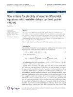
The trajectory of (5.1) with the initial function φ(θ) = cos 2θ − 1 is shown in the point
A(1.1,−0.9), which belongs to the summability region, on Figure 5.3 with η(t) ≡ 0and
on Figure 5.4 with η(t) described above. The trajectory of (5.1) with the initial func-
tion φ(θ) = 0.05cos2θ is shown in the point B(−0.5, 0.6), which does not belong to the
summability region, on Figure 5.5 with η(t) ≡ 0andonFigure 5.6 with η(t)described
above. The points A and B are shown on Figure 5.1.
Example 5.2. Consider the difference equation
x(t +1)= η(t +1)+ax(t)+
[t]+r

j=1
b
j
x(t − j), t>−1,
x(θ) = φ(θ), θ ∈

− (r +1),0

, r ≥ 0.
(5.14)
From condition (4.1), it follows that the inequality
|a| <
1 − 2|b|
1 −|b|
, |b| <
1
2

, (5.15)
is a sufficient condition for uniformly mean square summability of the solution of (5.14).
Condition (4.5)givesusasufficient condition for uniformly mean square summability
of the solution of (5.14)intheform
|a| <

1 − 2|b|
1 −|b|

1 − b
1 −|b|

, |b| <
1
2
. (5.16)
From (4.8), (4.10), and (4.11), we obtain another sufficient condition for uniformly mean
square summability of the solution of (5.14):
|b|
3
1 −|b|
<

β
2
2
+ d
−1
33
− β

2
, |b| < 1,
β
2
= b
2
+


a + b
3


+(1− b)


b(1 + ab)




1 − b − b
2

a + b
2



,

d
−1
33
= 1 − a
2
− b
2
− b
4
− 2b
b
2

a + b
3

+ a

a + b
2

(1 + ab)
1 − b − b
2

a + b
2

.
(5.17)

Using Mathematica program for solution of the matrix equation (3.5), sufficient con-
dition (3.31) for uniformly mean square summability of the solution of (5.14)wasob-
tained also for k
= 3andk = 4. In particular, for k = 3, this condition takes the form
b
4
1 −|b|
<

β
2
3
+ d
−1
44
− β
3
, |b| < 1,
β
3
=


b
3


+





a +
d
34
d
44




+




b +
d
24
d
44




+





b
2
+
d
14
d
44




,
(5.18)
86 Difference Volterra equations with continuous time
−210203040506070
t
−2
−1
1
2
x
Figure 5.4
−210203040506070
t
−2
−1
1
2
x
Figure 5.5

where
d
14
d
44
= b
3

b
3
+ b
5
− b
8
+ a

1 − b
3
+ b
4

G
−1
,
d
24
d
44
= b
2


a
2
b + b
2
+ b
5
− b
6
− b
8
+ a

1+b
4
+ b
6

G
−1
,
d
34
d
44
= b

b
2
+ a

3
b
2
+ b
4
− b
7
+ a
2

b + b
4

+ a

1+2b
3
+ b
5
− b
6
− b
8

G
−1
,
d
44
= G


1 − b − b
2
− a
4
b
3
− 2b
4
+2b
7
− 2b
8
+2b
9
− b
10
− b
12
+ b
13
− b
14
+ b
17
− a
3

b
2

+ b
5

− a
2

1+b +5b
4
− b
5
+ b
6
− 2b
7
− b
9

− ab
2

1+4b − b
2
+5b
3
− b
4
+ b
5
− 4b
6

+4b
7
− b
10
+ b
11

−1
,
G = 1 − b − ab
2
−

1+a
2

b
3
− b
4
− ab
5
− b
6
+ b
7
+ b
9
.
(5.19)

Leonid Shaikhet 87
−2 10203040
t
−4
−2
2
4
x
Figure 5.6
−0.4
a
1
0
−1
0.4
b
Figure 5.7
Condition (3.45)for(5.14) takes the form
−
1 − 3|b|
(1 − b)

1 −|b|

<a<
1 − 2b
1 − b
, |b| < 1. (5.20)
On Figure 5.7, the regions of uniformly mean square summability of the solution of
(5.14) are shown, obtained by condition (3.31). For k = 0 (condition (5.15), the brown

curve), for k = 1 (condition (5.16), the blue curve), for k = 2 (condition (5.17), the green
curve), for k = 3 (condition (5.18), the cyan curve), for k = 4 (the red curve) and also
obtained by condition (5.20) (the magenta curve).
As it is shown on Figure 5.7 (and naturally it can be shown analytically), for b ≥ 0
condition (5.15) coincides with condition (5.16)and,fora ≥ 0, b ≥ 0, conditions (5.15),
(5.16), (5.17), and (5.18) give the same region of uniformly mean square summability,
88 Difference Volterra equations with continuous time
−2
a
1
−1
−10
b
A
B
Figure 5.8
−2102030405060708090
t
−1
1
x
Figure 5.9
which is defined by the inequality
a +
b
1 − b
< 1, b<1. (5.21)
Note also that the region of uniformly mean square summability Q
k
of the solution

of (5.14), obtained by condition (3.31), expands if k increases, that is, Q
0
⊂ Q
1
⊂ Q
2
⊂
Q
3
⊂ Q
4
. So, to get a greater region of uniformly mean square summability, one can use
condition (3.31)fork = 5, k = 6, and so forth. But it is clear that each region Q
k
can be
obtained by the condition |b| < 1only.
Leonid Shaikhet 89
−2102030405060708090
t
−1
1
x
Figure 5.10
−2 10203040506070
t
−1
1
x
Figure 5.11
−21020304050

t
−3
−2
−1
1
2
3
x
Figure 5.12
90 Difference Volterra equations with continuous time
To obtain a condition of another t ype for uniformly mean square summability of the
solution of (5.14), transform the sum from (5.14)fort>0 in the following way :
[t]+r

j=1
b
j
x(t − j) = b
[t]+r

j=1
b
j−1
x(t − j)
= b
[t]−1+r

j=0
b
j

x(t − 1 − j)
= b


x(t − 1) +
[t]−1+r

j=1
b
j
x(t − 1 − j)


= b

(1 − a)x(t − 1) + x(t) − η(t)

.
(5.22)
Substituting (5.22)into(5.14), we obtain (5.14)intheform
x(t +1)= η(t +1)+ax(t)+
r−1

j=1
b
j
x(t − j), t ∈ (−1,0],
x(t +1)= η
1
(t +1)+(a + b)x(t)+b(1 − a)x(t − 1),

η
1
(t +1)= η(t +1)− bη(t), t>0.
(5.23)
The corresponding matrix D is defined by (4.3)witha
0
= a + b, a
1
= b(1 − a), and it
is a positive semidefinite one if and only if


b(1 − a)


< 1, |a + b| < 1 − b(1 − a). (5.24)
On Figure 5.8 the graph on Figure 5.7 is shown together with the region of uniformly
mean square summability obtained by condition (5.24)(theyellowcurve).
The trajectory of (5.14)withr = 1 and the initial functional φ(θ) = 0.8cosθ is shown
in the point A(1.2,−1.8), which belongs to the summability region, on Figure 5.9 with
η(t) ≡ 0andonFigure 5.10 with η(t) described above. The trajectory of (5.14)withr = 1
and the initial functional φ(θ) = 0.1cosθ is shown in the point B(1.33,−1.8), which does
not belong to the summability reg ion, on Figure 5.11 with η(t) ≡ 0andonFigure 5.12
with η(t) described above. The points A and B are shown on Figure 5.8.
References
[1] M. G. Blizorukov, On the c onstruction of solutions of linear difference systems with continuous
time,Differ. Uravn. 32 (1996), no. 1, 127–128, (Russian), translated in Differential Equa-
tions 32 (1996), no. 1, 133–134.
[2] V.B.Kolmanovski
˘

ı, The stability of certain discrete-time Volterra equations,J.Appl.Math.Mech.
63 (1999), no. 4, 537–543.
[3] V. B. Kolmanovski
˘
ı and A. Myshkis, Applied Theory of Functional-D ifferential Equations,Math-
ematics and Its Applications (Soviet Series), vol. 85, Kluwer Academic Publishers, Dor-
drecht, 1992.
[4] V. B. Kolmanovski
˘
ı and V. R. Nosov, Stability of Functional-Differential Equations,Mathematics
in Science and Engineering, vol. 180, Academic Press, London, 1986.
Leonid Shaikhet 91
[5] V. B. Kolmanovski
˘
ı and L. E. Shaikhet, New results in stability theory for stochastic functional-
differential equations (SFDEs) and their applications, Proceedings of Dynamic Systems and
Applications, Vol. 1 (Atlanta, Ga, 1993), Dynamic Publishers, Georgia, 1994, pp. 167–171.
[6]
, General method of Lyapunov functionals construction for stability investigation of sto-
chastic difference equations, Dynamical Systems and Applications, World Sci. Ser. Appl.
Anal., vol. 4, World Scientific Publishing, New Jersey, 1995, pp. 397–439.
[7] , A method for constructing Lyapunov functionals for stochastic differential equations of
neutral type,Differ. Uravn. 31 (1995), no. 11, 1851–1857 (Russian), translated in Differen-
tial Equations 31 (1996), no. 11, 1819–1825.
[8] , Control of Systems with Aftereffect, Translations of Mathematical Monographs, vol.
157, American Mathematical Society, Rhode Island, 1996.
[9] , Matrix Riccati equations and stability of stochastic linear systems with nonincreasing
delays, Funct. Differ. Equ. 4 (1997), no. 3-4, 279–293.
[10] , Riccati equations and stability of stochastic linear syste ms with distributed delay,Ad-
vances in Systems, Signals, Control and Computers (V. Bajic, ed.), vol. 1, IAAMSAD and

SA branch of the Academy of Nonlinear Sciences, Durban, 1998, pp. 97–100.
[11]
, Construction of Lyapunov functionals for stochastic hereditary systems: a survey of some
recent results, Math. Comput. Modelling 36 (2002), no. 6, 691–716.
[12] , Some peculiarities of the general method of Lyapunov functionals construction,Appl.
Math. Lett. 15 (2002), no. 3, 355–360.
[13] , About one application of the ge neral method of Lyapunov functionals construction,In-
ternational Journal of Robust and Nonlinear Control 13 (2003), no. 9, 805–818.
[14] D. G. Korenevski
˘
ı, Criteria for the stability of systems of linear deterministic and stochastic differ-
ence equations with continuous time and with delay, Mat. Zametki 70 (2001), no. 2, 213–229
(Russian), translated in Math. Notes 70 (2001), no. 1-2, 192–205.
[15] H. P
´
eics, Representation of solutions of difference equations with c ontinuous time, Proceedings of
the 6th Colloquium on the Qualitative Theory of Differential Equations (Szeged, 1999),
Proc. Colloq. Qual. Theory Differ.Equ.,no.21,Electron.J.Qual.TheoryDiffer. Equ.,
Szeged, 2000, pp. 1–8.
[16] G. P. Pelyukh, Representation of solutions of difference equations with a continuous argument,
Differ. U ravn. 32 (1996), no. 2, 256–264 (Russian), translated in Differential Equations 32
(1996), no. 2, 260–268.
[17] L. E. Shaikhet, Stability in probability of nonlinear stochastic hereditary systems,Dynam.Systems
Appl. 4 (1995), no. 2, 199–204.
[18]
, Modern state and development perspectives of Lyapunov functionals method in the sta-
bility theory of stochastic hereditary systems, Theory of Stochastic Processes 2(18) (1996),
no. 1-2, 248–259.
[19]
, Necessary and sufficient conditions of asymptotic mean square stability for stochastic

linear difference equations, Appl. Math. Lett. 10 (1997), no. 3, 111–115.
[20] A. N. Sharkovsky and Yu. L. Ma
˘
ıstrenko, Difference equations with continuous time as mathe-
matical models of the structure emergences, Dynamical Systems and Environmental Models
(Eisenach, 1986), Math. Ecol., Akademie-Verlag, Berlin, 1987, pp. 40–49.
[21] V. Volterra, Lec¸ons sur la Th
´
eorie Math
´
ematique de la Lutte pour la Vie, Gauthier-Villars, Paris,
1931.
Leonid Shaikhet: Department of Mathematics, Informatics, and Computing, Donetsk State Acad-
emy of Management, 163a Chelyuskintsev street, Donetsk 83015, Ukraine
E-mail address: