Báo cáo khoa học: "Stochastic Gradient Descent Training for L1-regularized Log-linear Models with Cumulative Penalty" potx
Bạn đang xem bản rút gọn của tài liệu. Xem và tải ngay bản đầy đủ của tài liệu tại đây (177.34 KB, 9 trang )
Proceedings of the 47th Annual Meeting of the ACL and the 4th IJCNLP of the AFNLP, pages 477–485,
Suntec, Singapore, 2-7 August 2009.
c
2009 ACL and AFNLP
Stochastic Gradient Descent Training for
L1-regularized Log-linear Models with Cumulative Penalty
Yoshimasa Tsuruoka
†‡
Jun’ichi Tsujii
†‡∗
Sophia Ananiadou
†‡
†
School of Computer Science, University of Manchester, UK
‡
National Centre for Text Mining (NaCTeM), UK
∗
Department of Computer Science, University of Tokyo, Japan
{yoshimasa.tsuruoka,j.tsujii,sophia.ananiadou}@manchester.ac.uk
Abstract
Stochastic gradient descent (SGD) uses
approximate gradients estimated from
subsets of the training data and updates
the parameters in an online fashion. This
learning framework is attractive because
it often requires much less training time
in practice than batch training algorithms.
However, L1-regularization, which is be-
coming popular in natural language pro-
cessing because of its ability to pro-
duce compact models, cannot be effi-
ciently applied in SGD training, due to
the large dimensions of feature vectors
and the fluctuations of approximate gra-
dients. We present a simple method to
solve these problems by penalizing the
weights according to cumulative values for
L1 penalty. We evaluate the effectiveness
of our method in three applications: text
chunking, named entity recognition, and
part-of-speech tagging. Experimental re-
sults demonstrate that our method can pro-
duce compact and accurate models much
more quickly than a state-of-the-art quasi-
Newton method for L1-regularized log-
linear models.
1 Introduction
Log-linear models (a.k.a maximum entropy mod-
els) are one of the most widely-used probabilistic
models in the field of natural language process-
ing (NLP). The applications range from simple
classification tasks such as text classification and
history-based tagging (Ratnaparkhi, 1996) to more
complex structured prediction tasks such as part-
of-speech (POS) tagging (Lafferty et al., 2001),
syntactic parsing (Clark and Curran, 2004) and se-
mantic role labeling (Toutanova et al., 2005). Log-
linear models have a major advantage over other
discriminative machine learning models such as
support vector machines—their probabilistic out-
put allows the information on the confidence of
the decision to be used by other components in the
text processing pipeline.
The training of log-liner models is typically per-
formed based on the maximum likelihood crite-
rion, which aims to obtain the weights of the fea-
tures that maximize the conditional likelihood of
the training data. In maximum likelihood training,
regularization is normally needed to prevent the
model from overfitting the training data,
The two most common regularization methods
are called L1 and L2 regularization. L1 regular-
ization penalizes the weight vector for its L1-norm
(i.e. the sum of the absolute values of the weights),
whereas L2 regularization uses its L2-norm. There
is usually not a considerable difference between
the two methods in terms of the accuracy of the
resulting model (Gao et al., 2007), but L1 regu-
larization has a significant advantage in practice.
Because many of the weights of the features be-
come zero as a result of L1-regularized training,
the size of the model can be much smaller than that
produced by L2-regularization. Compact models
require less space on memory and storage, and en-
able the application to start up quickly. These mer-
its can be of vital importance when the application
is deployed in resource-tight environments such as
cell-phones.
A common way to train a large-scale L1-
regularized model is to use a quasi-Newton
method. Kazama and Tsujii (2003) describe a
method for training a L1-regularized log-linear
model with a bound constrained version of the
BFGS algorithm (Nocedal, 1980). Andrew and
Gao (2007) present an algorithm called Orthant-
Wise Limited-memory Quasi-Newton (OWL-
QN), which can work on the BFGS algorithm
without bound constraints and achieve faster con-
vergence.
477
An alternative approach to training a log-linear
model is to use stochastic gradient descent (SGD)
methods. SGD uses approximate gradients esti-
mated from subsets of the training data and up-
dates the weights of the features in an online
fashion—the weights are updated much more fre-
quently than batch training algorithms. This learn-
ing framework is attracting attention because it of-
ten requires much less training time in practice
than batch training algorithms, especially when
the training data is large and redundant. SGD was
recently used for NLP tasks including machine
translation (Tillmann and Zhang, 2006) and syn-
tactic parsing (Smith and Eisner, 2008; Finkel et
al., 2008). Also, SGD is very easy to implement
because it does not need to use the Hessian infor-
mation on the objective function. The implemen-
tation could be as simple as the perceptron algo-
rithm.
Although SGD is a very attractive learning
framework, the direct application of L1 regular-
ization in this learning framework does not result
in efficient training. The first problem is the inef-
ficiency of applying the L1 penalty to the weights
of all features. In NLP applications, the dimen-
sion of the feature space tends to be very large—it
can easily become several millions, so the appli-
cation of L1 penalty to all features significantly
slows down the weight updating process. The sec-
ond problem is that the naive application of L1
penalty in SGD does not always lead to compact
models, because the approximate gradient used at
each update is very noisy, so the weights of the
features can be easily moved away from zero by
those fluctuations.
In this paper, we present a simple method for
solving these two problems in SGD learning. The
main idea is to keep track of the total penalty and
the penalty that has been applied to each weight,
so that the L1 penalty is applied based on the dif-
ference between those cumulative values. That
way, the application of L1 penalty is needed only
for the features that are used in the current sample,
and also the effect of noisy gradient is smoothed
away.
We evaluate the effectiveness of our method
by using linear-chain conditional random fields
(CRFs) and three traditional NLP tasks, namely,
text chunking (shallow parsing), named entity
recognition, and POS tagging. We show that our
enhanced SGD learning method can produce com-
pact and accurate models much more quickly than
the OWL-QN algorithm.
This paper is organized as follows. Section 2
provides a general description of log-linear mod-
els used in NLP. Section 3 describes our stochastic
gradient descent method for L1-regularized log-
linear models. Experimental results are presented
in Section 4. Some related work is discussed in
Section 5. Section 6 gives some concluding re-
marks.
2 Log-Linear Models
In this section, we briefly describe log-linear mod-
els used in NLP tasks and L1 regularization.
A log-linear model defines the following prob-
abilistic distribution over possible structure y for
input x:
p(y|x) =
1
Z(x)
exp
i
w
i
f
i
(y, x),
where f
i
(y, x) is a function indicating the occur-
rence of feature i, w
i
is the weight of the feature,
and Z(x) is a partition (normalization) function:
Z(x) =
y
exp
i
w
i
f
i
(y, x).
If the structure is a sequence, the model is called
a linear-chain CRF model, and the marginal prob-
abilities of the features and the partition function
can be efficiently computed by using the forward-
backward algorithm. The model is used for a va-
riety of sequence labeling tasks such as POS tag-
ging, chunking, and named entity recognition.
If the structure is a tree, the model is called a
tree CRF model, and the marginal probabilities
can be computed by using the inside-outside algo-
rithm. The model can be used for tasks like syn-
tactic parsing (Finkel et al., 2008) and semantic
role labeling (Cohn and Blunsom, 2005).
2.1 Training
The weights of the features in a log-linear model
are optimized in such a way that they maximize
the regularized conditional log-likelihood of the
training data:
L
w
=
N
j=1
log p(y
j
|x
j
; w) − R(w), (1)
where N is the number of training samples, y
j
is
the correct output for input x
j
, and R(w) is the
478
regularization term which prevents the model from
overfitting the training data. In the case of L1 reg-
ularization, the term is defined as:
R(w) = C
i
|w
i
|,
where C is the meta-parameter that controls the
degree of regularization, which is usually tuned by
cross-validation or using the heldout data.
In what follows, we denote by L(j, w)
the conditional log-likelihood of each sample
log p(y
j
|x
j
; w). Equation 1 is rewritten as:
L
w
=
N
j=1
L(j, w) − C
i
|w
i
|. (2)
3 Stochastic Gradient Descent
SGD uses a small randomly-selected subset of the
training samples to approximate the gradient of
the objective function given by Equation 2. The
number of training samples used for this approx-
imation is called the batch size. When the batch
size is N, the SGD training simply translates into
gradient descent (hence is very slow to converge).
By using a small batch size, one can update the
parameters more frequently than gradient descent
and speed up the convergence. The extreme case
is a batch size of 1, and it gives the maximum
frequency of updates and leads to a very simple
perceptron-like algorithm, which we adopt in this
work.
1
Apart from using a single training sample to
approximate the gradient, the optimization proce-
dure is the same as simple gradient descent,
2
so
the weights of the features are updated at training
sample j as follows:
w
k+1
= w
k
+ η
k
∂
∂w
(L(j, w) −
C
N
i
|w
i
|),
where k is the iteration counter and η
k
is the learn-
ing rate, which is normally designed to decrease
as the iteration proceeds. The actual learning rate
scheduling methods used in our experiments are
described later in Section 3.3.
1
In the actual implementation, we randomly shuffled the
training samples at the beginning of each pass, and then
picked them up sequentially.
2
What we actually do here is gradient ascent, but we stick
to the term “gradient descent”.
3.1 L1 regularization
The update equation for the weight of each feature
i is as follows:
w
i
k+1
= w
i
k
+ η
k
∂
∂w
i
(L(j, w) −
C
N
|w
i
|).
The difficulty with L1 regularization is that the
last term on the right-hand side of the above equa-
tion is not differentiable when the weight is zero.
One straightforward solution to this problem is to
consider a subgradient at zero and use the follow-
ing update equation:
w
i
k+1
= w
i
k
+ η
k
∂L(j, w)
∂w
i
−
C
N
η
k
sign(w
k
i
),
where sign(x) = 1 if x > 0, sign(x) = −1 if x <
0, and sign(x) = 0 if x = 0. In this paper, we call
this weight updating method “SGD-L1 (Naive)”.
This naive method has two serious problems.
The first problem is that, at each update, we need
to perform the application of L1 penalty to all fea-
tures, including the features that are not used in
the current training sample. Since the dimension
of the feature space can be very large, it can sig-
nificantly slow down the weight update process.
The second problem is that it does not produce
a compact model, i.e. most of the weights of the
features do not become zero as a result of train-
ing. Note that the weight of a feature does not be-
come zero unless it happens to fall on zero exactly,
which rarely happens in practice.
Carpenter (2008) describes an alternative ap-
proach. The weight updating process is divided
into two steps. First, the weight is updated with-
out considering the L1 penalty term. Then, the
L1 penalty is applied to the weight to the extent
that it does not change its sign. In other words,
the weight is clipped when it crosses zero. Their
weight update procedure is as follows:
w
k+
1
2
i
= w
k
i
+ η
k
∂L(j, w)
∂w
i
w=w
k
,
if w
k+
1
2
i
> 0 then
w
k+1
i
= max(0, w
k+
1
2
i
−
C
N
η
k
),
else if w
k+
1
2
i
< 0 then
w
k+1
i
= min(0, w
k+
1
2
i
+
C
N
η
k
).
In this paper, we call this update method “SGD-
L1 (Clipping)”. It should be noted that this method
479
-0.1
-0.05
0
0.05
0.1
0 1000 2000 3000 4000 5000 6000
Weight
Updates
Figure 1: An example of weight updates.
is actually a special case of the FOLOS algorithm
(Duchi and Singer, 2008) and the truncated gradi-
ent method (Langford et al., 2009).
The obvious advantage of using this method is
that we can expect many of the weights of the
features to become zero during training. Another
merit is that it allows us to perform the applica-
tion of L1 penalty in a lazy fashion, so that we
do not need to update the weights of the features
that are not used in the current sample, which leads
to much faster training when the dimension of the
feature space is large. See the aforementioned pa-
pers for the details. In this paper, we call this effi-
cient implementation “SGD-L1 (Clipping + Lazy-
Update)”.
3.2 L1 regularization with cumulative
penalty
Unfortunately, the clipping-at-zero approach does
not solve all problems. Still, we often end up with
many features whose weights are not zero. Re-
call that the gradient used in SGD is a crude ap-
proximation to the true gradient and is very noisy.
The weight of a feature is, therefore, easily moved
away from zero when the feature is used in the
current sample.
Figure 1 gives an illustrative example in which
the weight of a feature fails to become zero. The
figure shows how the weight of a feature changes
during training. The weight goes up sharply when
it is used in the sample and then is pulled back
toward zero gradually by the L1 penalty. There-
fore, the weight fails to become zero if the feature
is used toward the end of training, which is the
case in this example. Note that the weight would
become zero if the true (fluctuationless) gradient
were used—at each update the weight would go
up a little and be pulled back to zero straightaway.
Here, we present a different strategy for apply-
ing the L1 penalty to the weights of the features.
The key idea is to smooth out the effect of fluctu-
ating gradients by considering the cumulative ef-
fects from L1 penalty.
Let u
k
be the absolute value of the total L1-
penalty that each weight could have received up
to the point. Since the absolute value of the L1
penalty does not depend on the weight and we are
using the same regularization constant C for all
weights, it is simply accumulated as:
u
k
=
C
N
k
t=1
η
t
. (3)
At each training sample, we update the weights
of the features that are used in the sample as fol-
lows:
w
k+
1
2
i
= w
k
i
+ η
k
∂L(j, w)
∂w
i
w=w
k
,
if w
k+
1
2
i
> 0 then
w
k+1
i
= max(0, w
k+
1
2
i
− (u
k
+ q
k−1
i
)),
else if w
k+
1
2
i
< 0 then
w
k+1
i
= min(0, w
k+
1
2
i
+ (u
k
− q
k−1
i
)),
where q
k
i
is the total L1-penalty that w
i
has actu-
ally received up to the point:
q
k
i
=
k
t=1
(w
t+1
i
− w
t+
1
2
i
). (4)
This weight updating method penalizes the
weight according to the difference between u
k
and
q
k−1
i
. In effect, it forces the weight to receive the
total L1 penalty that would have been applied if
the weight had been updated by the true gradients,
assuming that the current weight vector resides in
the same orthant as the true weight vector.
It should be noted that this method is basi-
cally equivalent to a “SGD-L1 (Clipping + Lazy-
Update)” method if we were able to use the true
gradients instead of the stochastic gradients.
In this paper, we call this weight updating
method “SGD-L1 (Cumulative)”. The implemen-
tation of this method is very simple. Figure 2
shows the whole SGD training algorithm with this
strategy in pseudo-code.
480
1: procedure TRAIN(C)
2: u ← 0
3: Initialize w
i
and q
i
with zero for all i
4: for k = 0 to MaxIterations
5: η ← LEARNINGRATE(k)
6: u ← u + ηC/N
7: Select sample j randomly
8: UPDATEWEIGHTS(j)
9:
10: procedure UPDATEWEIGHTS(j)
11: for i ∈ features used in sample j
12: w
i
← w
i
+ η
∂L(j,w)
∂w
i
13: APPLYPENALTY(i)
14:
15: procedure APPLYPENALTY(i)
16: z ← w
i
17: if w
i
> 0 then
18: w
i
← max(0, w
i
− (u + q
i
))
19: else if w
i
< 0 then
20: w
i
← min(0, w
i
+ (u − q
i
))
21: q
i
← q
i
+ (w
i
− z)
22:
Figure 2: Stochastic gradient descent training with
cumulative L1 penalty. z is a temporary variable.
3.3 Learning Rate
The scheduling of learning rates often has a major
impact on the convergence speed in SGD training.
A typical choice of learning rate scheduling can
be found in (Collins et al., 2008):
η
k
=
η
0
1 + k/N
, (5)
where η
0
is a constant. Although this scheduling
guarantees ultimate convergence, the actual speed
of convergence can be poor in practice (Darken
and Moody, 1990).
In this work, we also tested simple exponential
decay:
η
k
= η
0
α
−k/N
, (6)
where α is a constant. In our experiments, we
found this scheduling more practical than that
given in Equation 5. This is mainly because ex-
ponential decay sweeps the range of learning rates
more smoothly—the learning rate given in Equa-
tion 5 drops too fast at the beginning and too
slowly at the end.
It should be noted that exponential decay is not
a good choice from a theoretical point of view, be-
cause it does not satisfy one of the necessary con-
ditions for convergence—the sum of the learning
rates must diverge to infinity (Spall, 2005). How-
ever, this is probably not a big issue for practition-
ers because normally the training has to be termi-
nated at a certain number of iterations in practice.
3
4 Experiments
We evaluate the effectiveness our training algo-
rithm using linear-chain CRF models and three
NLP tasks: text chunking, named entity recogni-
tion, and POS tagging.
To compare our algorithm with the state-of-the-
art, we present the performance of the OWL-QN
algorithm on the same data. We used the publicly
available OWL-QN optimizer developed by An-
drew and Gao.
4
The meta-parameters for learning
were left unchanged from the default settings of
the software: the convergence tolerance was 1e-4;
and the L-BFGS memory parameter was 10.
4.1 Text Chunking
The first set of experiments used the text chunk-
ing data set provided for the CoNLL 2000 shared
task.
5
The training data consists of 8,936 sen-
tences in which each token is annotated with the
“IOB” tags representing text chunks such as noun
and verb phrases. We separated 1,000 sentences
from the training data and used them as the held-
out data. The test data provided by the shared task
was used only for the final accuracy report.
The features used in this experiment were uni-
grams and bigrams of neighboring words, and un-
igrams, bigrams and trigrams of neighboring POS
tags.
To avoid giving any advantage to our SGD al-
gorithms over the OWL-QN algorithm in terms of
the accuracy of the resulting model, the OWL-QN
algorithm was used when tuning the regularization
parameter C. The tuning was performed in such a
way that it maximized the likelihood of the heldout
data. The learning rate parameters for SGD were
then tuned in such a way that they maximized the
value of the objective function in 30 passes. We
first determined η
0
by testing 1.0, 0.5, 0.2, and 0.1.
We then determined α by testing 0.9, 0.85, and 0.8
with the fixed η
0
.
3
This issue could also be sidestepped by, for example,
adding a small O(1/k) term to the learning rate.
4
Available from the original developers’ websites:
or
/>5
/>481
Passes L
w
/N # Features Time (sec) F-score
OWL-QN 160 -1.583 18,109 598 93.62
SGD-L1 (Naive)
30 -1.671 455,651 1,117 93.64
SGD-L1 (Clipping + Lazy-Update)
30 -1.671 87,792 144 93.65
SGD-L1 (Cumulative)
30 -1.653 28,189 149 93.68
SGD-L1 (Cumulative + Exponential-Decay)
30 -1.622 23,584 148 93.66
Table 1: CoNLL-2000 Chunking task. Training time and accuracy of the trained model on the test data.
-2.4
-2.2
-2
-1.8
-1.6
0 10 20 30 40 50
Objective function
Passes
OWL-QN
SGD-L1 (Clipping)
SGD-L1 (Cumulative)
SGD-L1 (Cumulative + ED)
Figure 3: CoNLL 2000 chunking task: Objective
0
50000
100000
150000
200000
0 10 20 30 40 50
# Active features
Passes
OWL-QN
SGD-L1 (Clipping)
SGD-L1 (Cumulative)
SGD-L1 (Cumulative + ED)
Figure 4: CoNLL 2000 chunking task: Number of
active features.
Figures 3 and 4 show the training process of
the model. Each figure contains four curves repre-
senting the results of the OWL-QN algorithm and
three SGD-based algorithms. “SGD-L1 (Cumu-
lative + ED)” represents the results of our cumu-
lative penalty-based method that uses exponential
decay (ED) for learning rate scheduling.
Figure 3 shows how the value of the objec-
tive function changed as the training proceeded.
SGD-based algorithms show much faster conver-
gence than the OWL-QN algorithm. Notice also
that “SGD-L1 (Cumulative)” improves the objec-
tive slightly faster than “SGD-L1 (Clipping)”. The
result of “SGD-L1 (Naive)” is not shown in this
figure, but the curve was almost identical to that
of “SGD-L1 (Clipping)”.
Figure 4 shows the numbers of active features
(the features whose weight are not zero). It is
clearly seen that the clipping-at-zero approach
fails to reduce the number of active features, while
our algorithms succeeded in reducing the number
of active features to the same level as OWL-QN.
We then trained the models using the whole
training data (including the heldout data) and eval-
uated the accuracy of the chunker on the test data.
The number of passes performed over the train-
ing data in SGD was set to 30. The results are
shown in Table 1. The second column shows the
number of passes performed in the training. The
third column shows the final value of the objective
function per sample. The fourth column shows
the number of resulting active features. The fifth
column show the training time. The last column
shows the f-score (harmonic mean of recall and
precision) of the chunking results. There was no
significant difference between the models in terms
of accuracy. The naive SGD training took much
longer than OWL-QN because of the overhead of
applying L1 penalty to all dimensions.
Our SGD algorithms finished training in 150
seconds on Xeon 2.13GHz processors. The
CRF++ version 0.50, a popular CRF library de-
veloped by Taku Kudo,
6
is reported to take 4,021
seconds on Xeon 3.0GHz processors to train the
model using a richer feature set.
7
CRFsuite ver-
sion 0.4, a much faster library for CRFs, is re-
ported to take 382 seconds on Xeon 3.0GHz, using
the same feature set as ours.
8
Their library uses the
OWL-QN algorithm for optimization. Although
direct comparison of training times is not impor-
6
/>7
/>8
ditto
482
tant due to the differences in implementation and
hardware platforms, these results demonstrate that
our algorithm can actually result in a very fast im-
plementation of a CRF trainer.
4.2 Named Entity Recognition
The second set of experiments used the named
entity recognition data set provided for the
BioNLP/NLPBA 2004 shared task (Kim et al.,
2004).
9
The training data consist of 18,546 sen-
tences in which each token is annotated with the
“IOB” tags representing biomedical named enti-
ties such as the names of proteins and RNAs.
The training and test data were preprocessed
by the GENIA tagger,
10
which provided POS tags
and chunk tags. We did not use any information on
the named entity tags output by the GENIA tagger.
For the features, we used unigrams of neighboring
chunk tags, substrings (shorter than 10 characters)
of the current word, and the shape of the word (e.g.
“IL-2” is converted into “AA-#”), on top of the
features used in the text chunking experiments.
The results are shown in Figure 5 and Table
2. The trend in the results is the same as that of
the text chunking task: our SGD algorithms show
much faster convergence than the OWL-QN algo-
rithm and produce compact models.
Okanohara et al. (2006) report an f-score of
71.48 on the same data, using semi-Markov CRFs.
4.3 Part-Of-Speech Tagging
The third set of experiments used the POS tag-
ging data in the Penn Treebank (Marcus et al.,
1994). Following (Collins, 2002), we used sec-
tions 0-18 of the Wall Street Journal (WSJ) corpus
for training, sections 19-21 for development, and
sections 22-24 for final evaluation. The POS tags
were extracted from the parse trees in the corpus.
All experiments for this work, including the tun-
ing of features and parameters for regularization,
were carried out using the training and develop-
ment sets. The test set was used only for the final
accuracy report.
It should be noted that training a CRF-based
POS tagger using the whole WSJ corpus is not a
trivial task and was once even deemed impractical
in previous studies. For example, Wellner and Vi-
lain (2006) abandoned maximum likelihood train-
9
The data is available for download at http://www-
tsujii.is.s.u-tokyo.ac.jp/GENIA/ERtask/report.html
10
/>-3.8
-3.6
-3.4
-3.2
-3
-2.8
-2.6
-2.4
-2.2
0 10 20 30 40 50
Objective function
Passes
OWL-QN
SGD-L1 (Clipping)
SGD-L1 (Cumulative)
SGD-L1 (Cumulative + ED)
Figure 5: NLPBA 2004 named entity recognition
task: Objective.
-2.8
-2.7
-2.6
-2.5
-2.4
-2.3
-2.2
-2.1
-2
-1.9
-1.8
0 10 20 30 40 50
Objective function
Passes
OWL-QN
SGD-L1 (Clipping)
SGD-L1 (Cumulative)
SGD-L1 (Cumulative + ED)
Figure 6: POS tagging task: Objective.
ing because it was “prohibitive” (7-8 days for sec-
tions 0-18 of the WSJ corpus).
For the features, we used unigrams and bigrams
of neighboring words, prefixes and suffixes of
the current word, and some characteristics of the
word. We also normalized the current word by
lowering capital letters and converting all the nu-
merals into ‘#’, and used the normalized word as a
feature.
The results are shown in Figure 6 and Table 3.
Again, the trend is the same. Our algorithms fin-
ished training in about 30 minutes, producing ac-
curate models that are as compact as that produced
by OWL-QN.
Shen et al., (2007) report an accuracy of 97.33%
on the same data set using a perceptron-based bidi-
rectional tagging model.
5 Discussion
An alternative approach to producing compact
models for log-linear models is to reformulate the
483
Passes L
w
/N # Features Time (sec) F-score
OWL-QN 161 -2.448 30,710 2,253 71.76
SGD-L1 (Naive)
30 -2.537 1,032,962 4,528 71.20
SGD-L1 (Clipping + Lazy-Update)
30 -2.538 279,886 585 71.20
SGD-L1 (Cumulative)
30 -2.479 31,986 631 71.40
SGD-L1 (Cumulative + Exponential-Decay)
30 -2.443 25,965 631 71.63
Table 2: NLPBA 2004 Named entity recognition task. Training time and accuracy of the trained model
on the test data.
Passes L
w
/N # Features Time (sec) Accuracy
OWL-QN 124 -1.941 50,870 5,623 97.16%
SGD-L1 (Naive)
30 -2.013 2,142,130 18,471 97.18%
SGD-L1 (Clipping + Lazy-Update)
30 -2.013 323,199 1,680 97.18%
SGD-L1 (Cumulative)
30 -1.987 62,043 1,777 97.19%
SGD-L1 (Cumulative + Exponential-Decay)
30 -1.954 51,857 1,774 97.17%
Table 3: POS tagging on the WSJ corpus. Training time and accuracy of the trained model on the test
data.
problem as a L1-constrained problem (Lee et al.,
2006), where the conditional log-likelihood of the
training data is maximized under a fixed constraint
of the L1-norm of the weight vector. Duchi et
al. (2008) describe efficient algorithms for pro-
jecting a weight vector onto the L1-ball. Although
L1-regularized and L1-constrained learning algo-
rithms are not directly comparable because the ob-
jective functions are different, it would be inter-
esting to compare the two approaches in terms
of practicality. It should be noted, however, that
the efficient algorithm presented in (Duchi et al.,
2008) needs to employ a red-black tree and is
rather complex.
In SGD learning, the need for tuning the meta-
parameters for learning rate scheduling can be an-
noying. In the case of exponential decay, the set-
ting of α = 0.85 turned out to be a good rule
of thumb in our experiments—it always produced
near best results in 30 passes, but the other param-
eter η
0
needed to be tuned. It would be very useful
if those meta-parameters could be tuned in a fully
automatic way.
There are some sophisticated algorithms for
adaptive learning rate scheduling in SGD learning
(Vishwanathan et al., 2006; Huang et al., 2007).
However, those algorithms use second-order infor-
mation (i.e. Hessian information) and thus need
access to the weights of the features that are not
used in the current sample, which should slow
down the weight updating process for the same
reason discussed earlier. It would be interesting
to investigate whether those sophisticated learning
scheduling algorithms can actually result in fast
training in large-scale NLP tasks.
6 Conclusion
We have presented a new variant of SGD that can
efficiently train L1-regularized log-linear models.
The algorithm is simple and extremely easy to im-
plement.
We have conducted experiments using CRFs
and three NLP tasks, and demonstrated empiri-
cally that our training algorithm can produce com-
pact and accurate models much more quickly than
a state-of-the-art quasi-Newton method for L1-
regularization.
Acknowledgments
We thank N. Okazaki, N. Yoshinaga, D.
Okanohara and the anonymous reviewers for their
useful comments and suggestions. The work de-
scribed in this paper has been funded by the
Biotechnology and Biological Sciences Research
Council (BBSRC; BB/E004431/1). The research
team is hosted by the JISC/BBSRC/EPSRC spon-
sored National Centre for Text Mining.
References
Galen Andrew and Jianfeng Gao. 2007. Scalable train-
ing of L1-regularized log-linear models. In Pro-
ceedings of ICML, pages 33–40.
484
Bob Carpenter. 2008. Lazy sparse stochastic gradient
descent for regularized multinomial logistic regres-
sion. Technical report, Alias-i.
Stephen Clark and James R. Curran. 2004. Parsing the
WSJ using CCG and log-linear models. In Proceed-
ings of COLING 2004, pages 103–110.
Trevor Cohn and Philip Blunsom. 2005. Semantic role
labeling with tree conditional random fields. In Pro-
ceedings of CoNLL, pages 169–172.
Michael Collins, Amir Globerson, Terry Koo, Xavier
Carreras, and Peter L. Bartlett. 2008. Exponen-
tiated gradient algorithms for conditional random
fields and max-margin markov networks. The Jour-
nal of Machine Learning Research (JMLR), 9:1775–
1822.
Michael Collins. 2002. Discriminative training meth-
ods for hidden markov models: Theory and exper-
iments with perceptron algorithms. In Proceedings
of EMNLP, pages 1–8.
Christian Darken and John Moody. 1990. Note on
learning rate schedules for stochastic optimization.
In Proceedings of NIPS, pages 832–838.
Juhn Duchi and Yoram Singer. 2008. Online and
batch learning using forward-looking subgradients.
In NIPS Workshop: OPT 2008 Optimization for Ma-
chine Learning.
Juhn Duchi, Shai Shalev-Shwartz, Yoram Singer, and
Tushar Chandra. 2008. Efficient projections onto
the l1-ball for learning in high dimensions. In Pro-
ceedings of ICML, pages 272–279.
Jenny Rose Finkel, Alex Kleeman, and Christopher D.
Manning. 2008. Efficient, feature-based, condi-
tional random field parsing. In Proceedings of ACL-
08:HLT, pages 959–967.
Jianfeng Gao, Galen Andrew, Mark Johnson, and
Kristina Toutanova. 2007. A comparative study of
parameter estimation methods for statistical natural
language processing. In Proceedings of ACL, pages
824–831.
Han-Shen Huang, Yu-Ming Chang, and Chun-Nan
Hsu. 2007. Training conditional random fields by
periodic step size adaptation for large-scale text min-
ing. In Proceedings of ICDM, pages 511–516.
Jun’ichi Kazama and Jun’ichi Tsujii. 2003. Evalua-
tion and extension of maximum entropy models with
inequality constraints. In Proceedings of EMNLP
2003.
J D. Kim, T. Ohta, Y. Tsuruoka, Y. Tateisi, and N. Col-
lier. 2004. Introduction to the bio-entity recognition
task at JNLPBA. In Proceedings of the International
Joint Workshop on Natural Language Processing in
Biomedicine and its Applications (JNLPBA), pages
70–75.
John Lafferty, Andrew McCallum, and Fernando
Pereira. 2001. Conditional random fields: Prob-
abilistic models for segmenting and labeling se-
quence data. In Proceedings of ICML, pages 282–
289.
John Langford, Lihong Li, and Tong Zhang. 2009.
Sparse online learning via truncated gradient. The
Journal of Machine Learning Research (JMLR),
10:777–801.
Su-In Lee, Honglak Lee, Pieter Abbeel, and Andrew Y.
Ng. 2006. Efficient l1 regularized logistic regres-
sion. In Proceedings of AAAI-06, pages 401–408.
Mitchell P. Marcus, Beatrice Santorini, and Mary Ann
Marcinkiewicz. 1994. Building a large annotated
corpus of English: The Penn Treebank. Computa-
tional Linguistics, 19(2):313–330.
Jorge Nocedal. 1980. Updating quasi-newton matrices
with limited storage. Mathematics of Computation,
35(151):773–782.
Daisuke Okanohara, Yusuke Miyao, Yoshimasa Tsu-
ruoka, and Jun’ichi Tsujii. 2006. Improving
the scalability of semi-markov conditional random
fields for named entity recognition. In Proceedings
of COLING/ACL, pages 465–472.
Adwait Ratnaparkhi. 1996. A maximum entropy
model for part-of-speech tagging. In Proceedings
of EMNLP 1996, pages 133–142.
Libin Shen, Giorgio Satta, and Aravind Joshi. 2007.
Guided learning for bidirectional sequence classifi-
cation. In Proceedings of ACL, pages 760–767.
David Smith and Jason Eisner. 2008. Dependency
parsing by belief propagation. In Proceedings of
EMNLP, pages 145–156.
James C. Spall. 2005. Introduction to Stochastic
Search and Optimization. Wiley-IEEE.
Christoph Tillmann and Tong Zhang. 2006. Adiscrim-
inative global training algorithm for statistical MT.
In Proceedings of COLING/ACL, pages 721–728.
Kristina Toutanova, Aria Haghighi, and Christopher
Manning. 2005. Joint learning improves semantic
role labeling. In Proceedings of ACL, pages 589–
596.
S. V. N. Vishwanathan, Nicol N. Schraudolph, Mark W.
Schmidt, and Kevin P. Murphy. 2006. Accelerated
training of conditional random fields with stochastic
gradient methods. In Proceedings of ICML, pages
969–976.
Ben Wellner and Marc Vilain. 2006. Leveraging
machine readable dictionaries in discriminative se-
quence models. In Proceedings of LREC 2006.
485