METHODS FOR DETERMINATION AND APPROXIMATION OF THE DOMAIN OF ATTRACTION IN THE CASE OF AUTONOMOUS pdf

METHODS FOR DETERMINATION AND APPROXIMATION
OF THE DOMAIN OF ATTRACTION IN THE CASE OF
AUTONOMOUS DISCRETE DYNAMICAL SYSTEMS
ST. BALINT, E. KASLIK, A. M. BALINT, AND A. GRIGIS
Received 15 October 2004; Accepted 18 October 2004
A method for determination and two methods for approximation of the domain of attrac-
tion D
a
(0) of the asymptotically stable zero steady state of an autonomous, R-analytical,
discrete dynamical system are presented. The method of determination is based on the
construction of a Lyapunov function V , whose domain of analyticity is D
a
(0). The first
method of approximation uses a sequence of Lyapunov functions V
p
, which converge to
the Lyapunov function V on D
a
(0). Each V
p
defines an estimate N
p
of D
a
(0). For any x ∈
D
a
(0), there exists an estimate N
p
x
which contains x. The second method of approxima-

tion uses a ball B(R)
⊂ D
a
(0) which generates the sequence of estimates M
p
= f
−p
(B(R)).
For any x
∈ D
a
(0), there exists an estimate M
p
x
which contains x. The cases ∂
0
f  < 1and
ρ(∂
0
f ) < 1 ≤∂
0
f  are treated separately because significant differences occur.
Copyright © 2006 Hindawi Publishing Corporation. All rights reserved.
1. Introduction
Let be the following discrete dynamical system:
x
k+1
= f

x

k

k = 0, 1,2, , (1.1)
where f : Ω
→ Ω is an R-analytic function defined on a domain Ω ⊂ R
n
,0∈ Ω and
f (0)
= 0, that is, x = 0 is a steady state (fixed point) of (1.1).
For r>0, denote by B(r)
={x ∈ R
n
: x <r} the ball of radius r.
The steady state x
= 0of(1.1) is “stable” provided that given any ball B(ε), there is a
ball B(δ)suchthatifx
∈ B(δ)then f
k
(x) ∈ B(ε), for k = 0,1,2, [4].
If in addition there is a ball B(r)suchthat f
k
(x) → 0ask →∞for all x ∈ B(r) then the
steady state x
= 0 is “asymptotically stable” [4].
The domain of attraction D
a
(0) of the asymptotically stable steady state x = 0 is the set
of initial states x
∈ Ω from which the system converges to the steady state itself, that is,
D

a
(0) =

x ∈ Ω | f
k
(x)
k→∞
−−−→ 0

. (1.2)
Hindawi Publishing Corporation
Advances in Difference Equations
Volume 2006, Ar ticle ID 23939, Pages 1–15
DOI 10.1155/ADE/2006/23939
2 Domains of attraction—dynamical systems
Theoretical research shows that the D
a
(0) and its boundary are complicated sets [5–9].
In most cases, they do not admit an explicit elementar y representation. The domain of
attraction of an asymptotically stable steady state of a discrete dynamical system is not
necessarily connected (which is the case for continuous dynamical systems). This fact is
shown by the following example.
Example 1.1. Let be the function f :
R →R defined by f (x)= (1/2)x − (1/4)x
2
+(1/2)x
3
+
(1/4)x
4

. The domain of attraction of the asymptotically stable steady state x = 0isD
a
(0) =
(−2.79,−2.46) ∪ (−1,1) which is not connected.
Different procedures are used for the approximation of the D
a
(0) with domains hav-
ing a simpler shape. For example, in the case of [4, Theorem 4.20, page 170] the domain
which approximates the D
a
(0) is defined by a Lyapunov function V built with the ma-
trix ∂
0
f of the linearized system in 0, under the assumption ∂
0
f  < 1. In [2], a Lya-
punov function V is presented in the case when the matrix ∂
0
f is a contraction, that
is,
∂
0
f  < 1. The Lyapunov function V is built using the whole nonlinear system, not
only the matrix ∂
0
f . V is defined on the whole D
a
(0), and more, the D
a
(0) is the nat-

ural domain of analyticity of V .In[3], this result is extended for the more gener a l case
when ρ(∂
0
f ) < 1(whereρ(∂
0
f ) denotes the spectral radius of ∂
0
f .) This last result is the
following.
Theorem 1.2 (see [3]). If the function f satisfies the following conditions:
f (0)
= 0,
ρ

∂
0
f

< 1,
(1.3)
then 0 is an asymptotically stable steady state. D
a
(0) is an open subset of Ω and coincides
w ith the natural domain of analyt icity of the unique solution V of the iterative first-order
functional equation
V

f (x)

−

V(x) =−x
2
,
V(0)
= 0.
(1.4)
The function V is positive on D
a
(0) and V(x)
x→x
0
→ +∞,foranyx
0
∈ ∂D
a
(0),(∂D
a
(0) de-
notes the boundar y of D
a
(0))orforx→∞.
The function V is given by
V(x)
=
∞

k=0


f

k
(x)


2
for any x ∈ D
a
(0). (1.5)
The Lyapunov function V can be found theoretically using relation (1.5). In the fol-
lowings, we will shortly present the procedure of determination and approximation of
the domain of attraction using the function V presented in [2, 3].
The region of convergence D
0
of the power series development of V in 0 is a part of the
domain of attraction D
a
(0). If D
0
is strictly contained in D
a
(0), then there exists a point
x
0
∈ ∂D
0
such that the function V is bounded on a neighborhood of x
0
.Letbethepower
St. Balint et al. 3
series development of V in x

0
. The domain of convergence D
1
of the series centered in x
0
gives a new part D
1
\ (D
0

D
1
) of the domain of attraction D
a
(0). At this step, the part
D
0

D
1
of D
a
(0) is obtained.
If there exists a point x
1
∈ ∂(D
0

D
1

) such that the function V is bounded on a neigh-
borhood of x
1
, then the domain D
0

D
1
is strictly included in the domain of attraction
D
a
(0). In this case, the procedure described above is repeated in x
1
.
The procedure cannot be continued in the case when it is found that on the boundary
of the domain D
0

D
1

···

D
p
obtained at step p, there are no points having neigh-
borhoods on which V is bounded.
This procedure gives an open connected estimate D of the domain of attraction D
a
(0).

Note that f
−k
(D), k ∈ N is also an estimate of D
a
(0), which is not necessarily connected.
The procedure described above is illustrated by the following examples.
Example 1.3. Let be the f :
R → R defined by f (x) = x
2
. Due to the equality f
k
(x) = x
2
k
the domain of attraction of the asy mptotically stable steady state x = 0isD
a
(0) = (−1,1).
TheLyapunovfunctionisV(x)
=

∞
k=0
x
2
k+1
. The domain of convergence of the series is
D
0
= (−1,1) which coincides with D
a

(0).
Example 1.4. Let b e the function f : Ω
= ( −∞,1) → Ω defined by f (x) = x/(e +(1− e)x).
Due to the equality f
k
(x) = x/(e
k
+(1− e
k
)x) the domain of attraction of the asymp-
totically stable steady state x
= 0isD
a
(0) = (−∞,1). The power ser ies expansion of the
Lyapunov function V(x)
=

∞
k=0
| f
k
(x)|
2
in 0 is
V(x)
=
∞

m=2
(m − 1)

∞

k=0
e
−2k

1 − e
−k

m−2
x
m
. (1.6)
The radius of convergence of the series (1.6)is
r
0
= lim
m→∞
m




(m − 1)
∞

k=0
e
−2k


1 − e
−k

m−2
= 1, (1.7)
therefore the domain of convergence of the series (1.6)isD
0
= (−1,1) ⊂ D
a
(0). More,
V(x)
→∞as x → 1andV(−1) < ∞. The radius of convergence of the power series ex-
pansion of V in
−1is
r
−1
= lim
m→∞
m





∞

k=1
e
k


e
k
− 1

m−2

(m − 3)e
k
+2


2e
k
− 1

m+2
= 1, (1.8)
therefore the domain of convergence of the power series development of V in
−1isD
−1
=
(−2,0) which gives a new part of D
a
(0).
Numerical results for more complex examples are given in [2, 3].
4 Domains of attraction—dynamical systems
2. Theoretical results when the matrix A
= ∂
0
f is a contraction (i.e., A < 1)

The function f can be written as
f (x)
= Ax +g(x)foranyx ∈ Ω, (2.1)
where A
=∂
0
f and g :Ω→Ω is an R-analytic function such that g(0)=0andlim
x→0
(g(x)
/x) = 0.
Proposition 2.1. If
A < 1, then there exists r>0 such that B(r) ⊂ Ω and  f (x) < x
for any x ∈ B(r) \{0}.
Proof. Due to the fact that lim
x→0
(g(x)/x) = 0 there exists r>0suchthatB(r) ⊂ Ω
and


g(x)


<

1 −A

x for any x ∈ B(r) \{0}. (2.2)
Let be x
∈ B(r) \{0}. Inequality (2.2)providesthat



f (x)


=


Ax + g(x)


≤
Ax +


g(x)


<


A +1−A

x=x (2.3)
therefore,
 f (x) < x. 
Definit ion 2.2. Let R>0bethelargestnumbersuchthatB(R) ⊂ Ω and  f (x) < x for
any x
∈ B(R) \{0}.
If for any r>0, B(r)
⊂ Ω and  f (x) < x for any x ∈ B(r) \{0},thenR = +∞ and

B(R)
= Ω =
R
n
.
Lemma 2.3. (a) B(R) is invariant to the flow of system (1.1).
(b) For any x
∈ B(R),thesequence( f
k
(x))
k∈N
is decreasing.
(c) For any p
≥ 0 and x ∈ B(R) \{0}, ΔV
p
(x) = V
p
( f (x)) − V
p
(x) < 0,where
V
p
(x) =
p

k=0


f
k

(x)


2
for x ∈ Ω. (2.4)
Proof. (a) If x
= 0, then f
k
(0) = 0, for any k ∈ N.Forx ∈ B(R) \{0},wehave f (x) <
x, which implies that f (x) ∈ B(R), that is, B(R) is invariant to the flow of system (1.1).
(b) By induction, it results that for x
∈ B(R)wehave f
k
(x) ∈ B(R)and f
k+1
(x)≤

f
k
(x), which means that the sequence ( f
k
(x))
k∈N
is decreasing.
(c) In particular, for p
≥ 0andx ∈ B(R), we have  f
p+1
(x)≤f (x) < x and
therefore, ΔV
p

(x) =f
p+1
(x)
2
−x
2
< 0. 
Corollary 2.4. For any p ≥ 0, there exists a maximal domain G
p
⊂ Ω such that 0 ∈ G
p
and for x ∈ G
p
\{0}, the (positive definite) function V
p
verifies ΔV
p
(x) < 0.Inotherwords,
for any p
≥ 0,thefunctionV
p
defined by (2.4)isaLyapunovfunctionfor(1.1)onG
p
.
Moreover, B(R)
⊂ G
p
for any p ≥ 0.
Theorem 2.5. B(R) is an invariant set included in the domain of att raction D
a

(0).
Proof. Let be x
∈ B(R) \{0}.Wehavetoprovethatlim
k→∞
f
k
(x) = 0.
St. Balint et al. 5
The sequence ( f
k
(x))
k∈N
is bounded: f
k
(x)belongstoB(R). Let be ( f
k
j
(x))
j∈N
acon-
vergent subsequence and let be lim
j→∞
f
k
j
(x) = y
0
. It is clear that y
0
∈ B(R).

It can be shown that


f
k
(x)


≥


y
0


for any k ∈ N. (2.5)
For this, observe first that f
k
j
(x) → y
0
and ( f
k
j
(x))
k∈N
is decreasing ( Lemma 2.3).
These imply that
 f
k

j
(x)≥y
0
 for any k
j
. On the other hand, for any k ∈ N,there
exists k
j
∈ N such that k
j
≥ k. Therefore, as the sequence ( f
k
(x))
k∈N
is decreasing
(Lemma 2.3), we obtain that
 f
k
(x)≥f
k
j
(x)≥y
0
.
We show now that y
0
= 0. Suppose the contrary, that is, y
0
= 0.
Inequality (2.5)becomes



f
k
(x)


≥


y
0


> 0foranyk ∈ N. (2.6)
By means of Lemma 2.3,wehavethat
 f (y
0
) < y
0
.
Therefore, there exists a neighborhood U
f (y
0
)
⊂ B(R)of f (y
0
)suchthatforanyz ∈
U
f (y

0
)
we have z < y
0
. On the other hand, for the neighborhood U
f (y
0
)
there ex-
ists a neighborhood U
y
0
⊂ B(R)ofy
0
such that for any y ∈ U
y
0
,wehave f (y) ∈ U
f (y
0
)
.
Therefore:


f (y)


<



y
0


for any y ∈ U
y
0
. (2.7)
As f
k
j
(x) → y
0
, there exists
¯
j such that f
k
j
(x) ∈ U
y
0
,forany j ≥
¯
j.Makingy
= f
k
j
(x)in
(2.7), it results that



f
k
j
+1
(x)


=


f

f
k
j
(x)



<


y
0


for j ≥
¯

j (2.8)
which contradicts (2.6). This means that y
0
= 0, consequently, every convergent subse-
quence of ( f
k
(x))
k∈N
converges to 0. This provides that the sequence ( f
k
(x))
k∈N
is con-
vergent to 0, and x
∈ D
a
(0).
Therefore, the ball B(R) is contained in the domain of attraction of D
a
(0). 
For p ≥ 0andc>0letbeN
c
p
the set
N
c
p
=

x ∈ Ω : V

p
(x) <c

. (2.9)
If c
= +∞,thenN
c
p
= Ω.
Theorem 2.6. Let be p
≥ 0 .Foranyc ∈ (0,(p +1)R
2
], the set N
c
p
is included in the domain
of attraction D
a
(0).
Proof. Let be c
∈ (0, (p +1)R
2
]andx ∈ N
c
p
.ThenV
p
(x) =

p

k
=0
 f
k
(x)
2
<c≤ (p +1)R
2
,
therefore, there exists k
∈{0,1, , p} such that  f
k
(x)
2
<R
2
. It results that f
k
(x) ∈
B(R) ⊂ D
a
(0), therefore, x ∈ D
a
(0). 
Remark 2.7. It is obvious that for p ≥ 0and0<c

<c

one has N
c


p
⊂ N
c

p
. Therefore, for
agivenp
≥ 0, the largest part of D
a
(0) which can be found by this method is N
c
p
p
,where
6 Domains of attraction—dynamical systems
c
p
= (p +1)R
2
. In the followings, we will use the notation N
p
instead of N
c
p
p
.Shortly,
N
p
={x ∈ Ω : V

p
(x) < (p +1)R
2
} is a part of D
a
(0). Let us note that N
0
= B(R).
Remark 2.8. If R
= +∞ (i.e., Ω =
R
n
and  f (x) < x,foranyx ∈ R \{0}), then N
p
=
R
n
for any p ≥ 0andD
a
(0) =
R
n
.
Theorem 2.9. For the sets (N
p
)
p∈N
, the following properties hold:
(a) for any p
≥ 0 , one has N

p
⊂ N
p+1
;
(b) for any p
≥ 0 , the set N
p
is invariant to f ;
(c) for any x
∈ D
a
(0),thereexistsp
x
≥ 0 such that x ∈ N
p
x
.
Proof. (a) Let be p
≥ 0andx ∈ N
p
.ThenV
p
(x) =

p
k
=0
 f
k
(x)

2
< (p +1)R
2
, therefore,
there exists k
∈{0,1, , p} such that  f
k
(x)
2
<R
2
. It results that f
k
(x) ∈ B(R)and
therefore f
m
(x) ∈ B(R), for any m ≥ k.Form = p +1 weobtain f
p+1
(x) <R,hence
V
p+1
(x) = V
p
(x)+ f
p+1
(x)
2
< (p +1)R
2
+ R

2
= (p +2)R
2
. Therefore, x ∈ N
p+1
.
(b) Let be x
∈ N
p
.Ifx <R then  f
m
(x) <R for any m ≥ 0(bymeansof
Lemma 2.3). This implies that V
p
( f (x)) =

p
k
=0
 f
k
( f (x))
2
=

p+1
k
=1
 f
k

(x)
2
< (p +
1)R
2
, meaning that f (x) ∈ N
p
.
Let us suppose that
x≥R.Asx ∈ N
p
,wehavethatV
p
(x) =

p
k
=0
 f
k
(x)
2
< (p +
1)R
2
, therefore, there exists k ∈{0,1, , p} such that  f
k
(x) <R. It results that f
k
(x) ∈

B(R) and therefore f
m
(x) ∈ B(R), for any m ≥ k.Form = p +1weobtain f
p+1
(x) <R.
This implies that
V
p

f (x)

=
V
p
(x)+


f
p+1
(x)


2
−x
2
< (p +1)R
2
+ R
2
− R

2
= (p +1)R
2
(2.10)
therefore f (x)
∈ N
p
.
(c) Suppose the contrary, that is, there exist x
∈ D
a
(0) such that for any p ≥ 0, x/∈
N
p
. Therefore, V
p
(x) ≥ (p +1)R
2
for any p ≥ 0. Passing to the limit for p →∞in this
inequality, provides that V (x)
=∞. This means x ∈ ∂D
a
(0) which contradicts the fact
that x belongs to the open set D
a
(0). In conclusion, there exists p
x
≥ 0suchthatx ∈
N
p

x
. 
For p ≥ 0letbeM
p
= f
−p
(B(R)) ={x ∈ Ω : f
p
(x) ∈ B(R)}, obtained by the trajectory
reversing method.
Theorem 2.10. The following properties hold:
(a) M
p
⊂ D
a
(0) for any p ≥ 0;
(b) for any p
≥ 0 , M
p
is invariant to f ;
(c) M
p
⊂ M
p+1
for any p ≥ 0;
(d) for any x
∈ D
a
(0),thereexistsp
x

≥ 0 such that x ∈ M
p
x
.
Proof. (a) As M
p
= f
−p
(B(R)) and B(R) ⊂ D
a
(0) (see Theorem 2.5)itisclearthatM
p
⊂
D
a
(0).
(b) and (c) follow easily by induction, using Lemma 2.3.
(d) x
∈ D
a
(0) provides that f
p
(x) → 0asp →∞. Therefore, there exists p
x
∈ N such
that f
p
(x) ∈ B(R), for any p ≥ p
x
. This provides that x ∈ M

p
for any p ≥ p
x
. 
St. Balint et al. 7
Both sequences of sets (M
p
)
p∈N
and (N
p
)
p∈N
are increasing, and are made up of esti-
mates of D
a
(0). From the practical point of view, it is important to know which sequence
converges more quickly. The next theorem provides that the sequence (M
p
)
p∈N
converges
more quickly than (N
p
)
p∈N
, meaning that for p ≥ 0, the set M
p
is a larger estimate of
D

a
(0) then N
p
.
Theorem 2.11. For any p
≥ 0 , one has N
p
⊂ M
p
.
Proof. Let be p
≥ 0andx ∈ N
p
.WehavethatV
p
(x) =

p
k
=0
 f
k
(x)
2
< (p +1)R
2
,there-
fore, there exists k
∈{0,1, , p} such that  f
k

(x) <R. This implies that f
m
(x) ∈ B(R),
for any m
≥ k.Form = p we obtain f
p
(x) ∈ B(R), meaning that x ∈ M
p
. 
3. Theoretical results when A = ∂
0
f is a convergent noncontractive matrix
(i.e., ρ(A) < 1
≤A)
Proposition 3.1. If ρ(A) < 1
≤A, then the re exist

p ≥ 2 and r

p
> 0 such that B(r

p
) ⊂ Ω
and
 f
p
(x) < x for any p ∈{

p,


p +1, ,2

p − 1} and x ∈ B(r

p
) \{0}.
Proof. We have that ρ(A) < 1ifandonlyiflim
p→∞
A
p
= 0 (see [1]), which provides (to-
gether with
A≥1) that there exists

p ≥ 2suchthatA
p
 < 1foranyp ≥

p.Letbe

p ≥ 2 fixed with this property.
The formula of variation of constants for any p gives:
f
p
(x) = A
p
x +
p−1


k=0
A
p−k−1
g

f
k
(x)

∀
x ∈ Ω, p ∈ N

. (3.1)
Due to the fact that for any k
∈ N we have lim
x→0
(g( f
k
(x))/x) = 0, there exists r

p
> 0
such that for any p
∈{

p,

p +1, ,2

p − 1} the following inequality holds:

p−1

k=0


A
p−k−1




g

f
k
(x)



<

1 −


A
p





x for x ∈ B

r

p

\{
0}. (3.2)
Let be x
∈ B(r

p
) \{0} and p ∈{

p,

p +1, ,2

p − 1}. Using (3.1)and(3.2)wehave


f
p
(x)


=






A
p
x +
p−1

k=0
A
p−k−1
g

f
k
(x)






≤


A
p



x +

p−1

k=0


A
p−k−1




g

f
k
(x)



<



A
p


+1−



A
p




x=x.
(3.3)
Therefore,
 f
p
(x) < x for p ∈{

p,

p +1, ,2

p − 1} and x ∈ B(r

p
) \{0}. 
Definit ion 3.2. Let

p ≥ 2 be the smallest number such that A
p
 < 1foranyp ≥

p (see
the proof of Proposition 3.1). Let


R>0thelargestnumberbesuchthatB(

R) ⊂ Ω and
 f
p
(x) < x for p ∈{

p,

p +1, ,2

p − 1} and x ∈ B(

R) \{0}.
8 Domains of attraction—dynamical systems
If for any r>0, we have that B(r)
⊂ Ω and  f
p
(x) < x for any p ∈{

p,

p +1, ,
2

p − 1} and x ∈ B(r) \{0},then

R = +∞ and B(

R) = Ω =

R
n
.
Lemma 3.3. (a) For any x
∈B(

R) and p ∈{

p,

p +1, ,2

p − 1},thesequence( f
kp
(x))
k∈N
is decreasing.
(b) For any p
≥

p and x ∈ B(

R) \{0},  f
p
(x) < x.
(c) For any p
≥

p and x ∈ B(


R) \{0}, ΔV
p
(x) = V
p
( f (x)) − V
p
(x) < 0,whereV
p
is
defined by (2.4).
Proof. (a) If x
= 0, then f
p
(0) = 0, for any p ≥ 0.
Let be x
∈ B(

R) \{0}.Weknowthat f
p
(x) < x for any p ∈{

p,

p +1, ,2

p − 1}.
It results that f
p
(x) ∈ B(


R)foranyp ∈{

p,

p +1, ,2

p − 1}. This implies t hat for any
k
∈ N

we have  f
kp
(x) < x and  f
(k+1)p
(x)≤f
kp
(x), meaning that the sequence
(
 f
kp
(x))
k∈N
is decreasing.
(b) Let be x
∈ B(

R) \{0}. Inequality  f
p
(x) < x is true for any p ∈{


p,

p +1, ,
2

p − 1}.
Let be p
≥ 2

p. There exists q ∈ N

and p

∈{

p,

p +1, ,2

p − 1} such that p = q

p +
p

. Using (a), we have that f
p

(x) ∈ B(

R)and f

q

p
(y) ≤y,foranyy ∈ B(

R), therefore


f
p
(x)


=


f
q

p

f
p

(x)



≤



f
p

(x)


< x (3.4)
(c) results directly from (b).

Corollary 3.4. For any p ≥

p, there exists a maximal domain G
p
⊂ Ω such that 0 ∈ G
p
and for any x ∈ G
p
\{0}, the (positive definite) function V
p
verifies ΔV
p
(x) < 0.Inother
words, for any p
≥

p,thefunctionV
p
is a Lyapunov function for (1.1)onG
p

.More,B(

R) ⊂
G
p
for any p ≥

p.
Lemma 3.5. For any k
≥

p,thereexistsq
k
∈ N such that


f
(q
k
+3)

p
(x)


≤


f
k

(x)


≤


f
q
k

p
(x)


for any x ∈ B


R

. (3.5)
Proof. Let be k
≥

p. There exists a unique q
k
∈ N and a unique p
k
∈{

p,


p +1, ,2

p − 1}
such that k = q
k

p + p
k
. Lemma 3.3 provides that for any x ∈ B(

R)wehavethat f
q
k

p
(x) ∈
B(

R)and f
p
k
(x)≤x. It results that


f
k
(x)



=


f
p
k

f
q
k

p
(x)



≤


f
q
k

p
(x)


for any x ∈ B

¯

R

. (3.6)
On the other hand, we have (q
k
+3)

p = k +(3

p − p
k
). As (3

p − p
k
) ∈{

p +1,

p +2, ,2

p}
and k ≥

p, Lemma 3.3 provides that for any x ∈ B(

R)wehavethat f
k
(x) ∈ B(


R)and
St. Balint et al. 9
 f
3

p−p
k
(x)≤x. Therefore


f
(q
k
+3)

p
(x)


=


f
3

p−p
k

f
k

(x)



≤


f
k
(x)


for any x ∈ B


R

. (3.7)
Combining the two inequalities, we get that


f
(q
k
+3)

p
(x)



≤


f
k
(x)


≤


f
q
k

p
(x)


for any x ∈ B


R

(3.8)
which concludes the proof.

Theorem 3.6. B(

R) is included in the domain of attraction D

a
(0).
Proof. Let be x
∈ B(

R) \{0}.Wehavetoprovethatlim
k→∞
f
k
(x) = 0.
The sequence ( f
k
(x))
k∈N
is bounded (see Lemma 3.3). Let be ( f
k
j
(x))
j∈N
aconvergent
subsequence and let be lim
j→∞
f
k
j
(x) = y
0
.
We suppose, without loss of generality, that k
j

≥

p for any j ∈ N. Lemma 3.5 provides
that for any j
∈ N there exists q
j
∈ N such that


f
(q
j
+3)

p
(x)


≤


f
k
j
(x)


≤



f
q
j

p
(x)


. (3.9)
As (
 f
q
j

p
(x))
j∈N
and ( f
(q
j
+3)

p
(x))
j∈N
are subsequences of the convergent sequence
(
 f
q


p
(x))
q∈N
(decreasing, according to Lemma 3.3), it results that they are convergent.
Thedoubleinequality(3.9) provides that lim
j→∞
 f
q
j

p
(x)=y
0
. Therefore, lim
q→∞
 f
q

p
(x)=y
0
.
It can be shown that


f
k
(x)



≥


y
0


for any k ≥

p. (3.10)
For this, remark that lim
q→∞
 f
q

p
(x)=y
0
 and ( f
q

p
(x))
q∈N
is decreasing (Lemma
3.3), which implies that
 f
q

p

(x)≥y
0
 for any q ∈ N. On the other hand, Lemma 3.5
provides that for any k
≥

p there exists q
k
such that  f
(q
k
+3)

p
(x)≤f
k
(x). Therefore,
 f
k
(x)≥f
(q
k
+3)

p
(x)≥y
0
,foranyk ≥

p.

We show now that y
0
= 0. Suppose the contrary, that is, y
0
= 0.
Inequality (3.10)becomes


f
k
(x)


≥


y
0


> 0foranyk ≥

p. (3.11)
By means of Lemma 3.3,wehavethat
 f

p
(y
0
) < y

0
.
There exists a neighborhood U
f

p
(y
0
)
⊂ B(

R)of f

p
(y
0
) such that for any z ∈ U
f

p
(y
0
)
we
have
z < y
0
. On the other hand, for the neighborhood U
f


p
(y
0
)
there exists a neigh-
borhood U
y
0
⊂ B(

R)ofy
0
such that for any y ∈ U
y
0
,wehave f

p
(y) ∈ U
f

p
(y
0
)
. Therefore:


f


p
(y)


<


y
0


for any y ∈ U
y
0
. (3.12)
10 Domains of attraction—dynamical systems
As f
k
j
(x) → y
0
, there exists
¯
j such that f
k
j
(x) ∈ U
y
0
,forany j ≥

¯
j.Makingy
= f
k
j
(x)in
(3.12), it results that


f
k
j
+

p
(x)


=


f

p

f
k
j
(x)




<


y
0


for j ≥
¯
j (3.13)
which contradicts (3.11). This means that y
0
= 0, consequently, every convergent sub-
sequence of ( f
k
(x))
k∈N
converges to 0. This provides that the s equence ( f
k
(x))
k∈N
is
convergent to 0, and x
∈ D
a
(0).
Therefore, the ball B(


R) is contained in the domain of attraction of D
a
(0). 
Theorem 3.7. Let be p ≥ 0.Foranyc ∈ (0,(p +1)

R
2
], the set N
c
p
is included in the domain
of attraction D
a
(0).
Proof. Let be c
∈ (0, (p +1)

R
2
]andx ∈ N
c
p
.ThenV
p
(x) =

p
k
=0
 f

k
(x)
2
<c≤ (p +1)

R
2
,
therefore, there exists k
∈{0,1, , p} such that  f
k
(x)
2
<

R
2
. It results that f
k
(x) ∈
B(

R) ⊂ D
a
(0), therefore, x ∈ D
a
(0). 
Remark 3.8. It is obvious that for p ≥ 0and0<c

<c


one has N
c

p
⊂ N
c

p
. Therefore, for
agivenp
≥ 0, the largest part of D
a
(0) which can be found by this method is N
c
p
p
,where
c
p
= (p +1)

R
2
. In the followings, we will use the notation

N
p
instead of N
c

p
p
.Shortly,

N
p
={x ∈ Ω : V
p
(x) < (p +1)

R
2
} is a part of D
a
(0). Let us note that

N
0
= B(

R).
Remark 3.9. If

R = +∞ (i.e., Ω =
R
n
and  f
p
(x) < x,foranyp ∈{


p,

p +1, ,2

p − 1}
and x ∈ R \{0}), then

N
p
=
R
n
for any p ≥ 0andD
a
(0) =
R
n
.
Theorem 3.10. For any x
∈ D
a
(0) there exists p
x
≥ 0 such that x ∈

N
p
x
.
Proof. Let be x

∈ D
a
(0). Suppose the contrary, that is, x/∈

N
p
for any p ≥ 0. Therefore,
V
p
(x) ≥ (p +1)

R
2
for any p ≥ 0. Passing to the limit when p →∞in this inequality pro-
vides that V (x)
=∞. This means x ∈ ∂D
a
(0) which contradicts the fact that x belongs to
the open set D
a
(0). In conclusion, there exists p
x
≥ 0suchthatx ∈

N
p
x
. 
Remark 3.11. Thesequenceofsets(


N
p
)
p∈N
is generally not increasing (see Section 4:
Numerical examples, the Van der Pol equation).
Open question. Is the sequence of sets (

N
p
)
p≥

p
increasing?
For p
≥ 0letbe

M
p
= f
−p
(B(

R)) ={x ∈ Ω : f
p
(x) ∈ B(

R)}, obtained by the trajectory
reversing method.

Theorem 3.12. For the sets (

M
p
)
p∈N
, the following properties hold:
(a)

M
p
⊂ D
a
(0),foranyp ≥ 0;
(b)

M
kp
⊂

M
(k+1)p
for any k ∈ N and p ∈{

p,

p +1, ,2

p − 1};
(c) for any x

∈ D
a
(0),thereexistsp
x
≥ 0 such that x ∈

M
p
x
.
Proof. (a) As

M
p
= f
−p
(B(

R)) and B(

R) ⊂ D
a
(0) (see Theorem 3.6)itisclearthat

M
p
⊂
D
a
(0).

(b) follows easily by induction, using Lemma 3.3.
(c) x
∈ D
a
(0) provides that f
p
(x) → 0asp →∞. Therefore, there exists p
x
≥ 0such
that f
p
(x) ∈ B(

R), for any p ≥ p
x
. This provides that x ∈

M
p
for any p ≥ p
x
. 
St.Balintetal. 11
−10.50−0.5−1
−1
−0.5
0
0.5
1
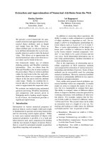
Figure 4.1. The sets N

p
, p = 0, 4 and ∂D
a
(0,0) for (4.1).
Remark 3.13. Thesequenceofsets(

M
p
)
p∈N
is generally not increasing (see Section 4:
Numerical examples, the Van der Pol equation).
Both sequences of sets (

M
p
)
p∈N
and (

N
p
)
p∈N
aremadeupofestimatesofD
a
(0). From
the practical point of view, it would be important to know which one of the sets

M

p
or

N
p
is a larger estimate of D
a
(0) for a fixed p ≥

p. Such result could not be established, but
the following theorem holds.
Theorem 3.14. For any p
≥ 0 , one has

N
p
⊂

M
p+

p
.
Proof. Let be p
≥ 0andx ∈

N
p
.WehavethatV
p

(x) =

p
k
=0
 f
k
(x)
2
< (p +1)

R
2
,there-
fore, there exists k
∈{0,1, , p} such that  f
k
(x) <

R. This implies that f
k+m
(x) ∈ B(

R),
for any m
≥

p.Form = p − k +

p we obtain f

p+

p
(x) ∈ B(

R), meaning that x ∈

M
p+

p
. 
4. Numerical examples
4.1. Example with known domain of attraction. Let the following discrete dynamical
system be
x
k+1
=
1
2
x
k

1+x
2
k
+2y
2
k


y
k+1
=
1
2
y
k

1+x
2
k
+2y
2
k

k ∈ N. (4.1)
There exists an infinity of steady states for this system: (0,0) (asymptotically stable) and
all the points (x, y) belonging to the ellipsis x
2
+2y
2
= 1 (all unstable). The domain of
attracti on of (0, 0) is D
a
(0,0) ={(x, y) ∈ R
2
: x
2
+2y
2

< 1 }.
12 Domains of attraction—dynamical systems
−10.50−0.5−1
−1
−0.5
0
0.5
1
Figure 4.2. The sets M
p
, p = 0, 1,2,6 for (4.1).
As ∂
(0,0)
f =1/2, we compute the largest number R>0suchthat f (x) < x for
any x
∈ B(R) \{0},andwefindR = 0.7071.
For p
= 0,1,2,3,4, we find the N
p
sets shown in Figure 4.1,partsofD
a
(0,0) (N
p
⊂
N
p+1
,forp ≥ 0). In Figure 4.1, the thick-contoured ellipsis represents the boundary of
D
a
(0,0).

In Figure 4.2, the sets M
p
are represented, for p = 0,1,2,6 (M
p
⊂ M
p+1
,forp ≥ 0).
Note that M
6
approximates with a good accuracy the domain of attraction.
4.2. Discrete predator-prey system. We consider the discrete predator-prey system:
x
k+1
= ax
k

1 − x
k

−
x
k
y
k
y
k+1
=
1
b
x

k
y
k
with a =
1
2
, b
= 1, k ∈ N. (4.2)
The steady states of this system are (0,0) (asymptotically stable), (
−1,0) and (1,−1) (both
unstable).
We have that
∂
(0,0)
f =1/2, and the largest number R>0suchthat f (x) < x for
any x
∈ B(R) \{0} is R = 0.65.
Figure 4.3 presents the N
p
sets for p = 0,1,2,3,4,5, parts of D
a
(0,0) (N
p
⊂ N
p+1
,for
p
≥ 0). The black points in Figure 4.3 represent the steady states of the system.
In Figure 4.4, the sets M
p

are represented, for p = 0,1,2,6 (M
p
⊂ M
p+1
,forp ≥ 0).
Note that the boundary of M
6
approaches very much the fixed points (−1, 0) and (1,−1),
which suggests that M
6
is a good approximation of D
a
(0).
St.Balintetal. 13
1.510.50−0.5−1
−1.5
−1
−0.5
0
0.5
1
1.5
Figure 4.3. The sets N
p
, p = 0, 5 for (4.2).
420−2−4
−4
−2
0
2

4
Figure 4.4. The sets M
p
, p = 0, 1,2,6 for (4.2).
4.3. Discrete Van der Pol system. Let the following discrete dynamical system, obtained
from the continuous Van der Pol system be
x
k+1
= x
k
− y
k
y
k+1
= x
k
+(1− a)y
k
+ ax
2
k
y
k
with a = 2, k ∈ N. (4.3)
14 Domains of attraction—dynamical systems
0.750.50.250−0.25−0.5−0.75
−1
−0.5
0
0.5

1
Figure 4.5. The sets

N
p
, p = 0, 5 for (4.3).
0.750.50.250−0.25−0.5−0.75
−1
−0.5
0
0.5
1
Figure 4.6. The sets

M
p
, p = 0, 1,2,6 for (4.3).
The only steady state of this system is (0,0) which is asymptotically stable. There are
many periodic points for this system, the periodic points of order
2,5 being represented
in Figure 4.5 by the black points.
We have that
∂
(0,0)
f =2butρ(∂
(0,0)
f ) = 0. First, we observe that for

p = 2wehave
that (∂

(0,0)
f )

p
= O
2
, therefore, (∂
(0,0)
f )
p
=0foranyp ≥

p.
St.Balintetal. 15
The largest number

R>0suchthat f
p
(x) < x for p ∈{

p,

p +1, ,2

p − 1}=
{
2,3} and x ∈ B(

R) \{0} is


R = 0.365.
For p
= 0,1,2, 3,4,5, the connected components which contain (0,0) of the

N
p
sets are
shown in Figure 4.5.Wehavethat

N
0


N
1
⊂

N
2
⊂

N
3
⊂

N
4
⊂

N

5
.
In Figure 4.6, the sets

M
p
are represented, for p = 0,1,2,6. Note that the inclusions

M
p
⊂

M
p+1
do not hold.
References
[1] R. A. Horn and C. R. Johnson, Matrix Analysis, Cambridge University Press, Cambridge, 1985.
[2] E. Kaslik, A. M. Balint, S. Birauas, and St. Balint, Approximation of the domain of attraction of an
asymptotically stable fixed point of a first order analytical system of difference equations, Nonlinear
Studies 10 (2003), no. 2, 103–112.
[3] E. Kaslik, A. M. Balint, A. Grigis, and St. Balint, An extension of the characterization of the domain
of attraction of an asymptotically stable fixed point in the case of a nonlinear discrete dynamical
system, Proceedings of 5th ICNPAA (S. Sivasundaram, ed.), European Conference Publications,
Cambridge, UK, 2004.
[4] W. G. Kelley and A. C. Peterson, Difference Equations, 2nd ed., Harcourt/Academic Press, Cali-
fornia, 2001.
[5] H. Koc¸ak, Differential and Difference Equations through Computer Experiments,2nded.,
Springer, New York, 1989.
[6] G.Ladas,C.Qian,P.N.Vlahos,andJ.Yan,Stability of solutions of linear nonautonomous differ-
ence equations, Applicable Analysis. An International Journal 41 (1991), no. 1-4, 183–191.

[7] V. Lakshmikantham and D. Trigiante, Theory of Difference Equations. Numerical Methods and
Applications, Mathematics in Science and Engineering, vol. 181, Academic Press, Massachusetts,
1988.
[8] J.P.LaSalle,The Stability and Control of Discrete Processes, Applied Mathematical Sciences, vol.
62, Springer, New York, 1986.
[9]
, Stability theory for difference equations, Studies in Ordinary Differntial Equations (J.
Hale, ed.), MAA Studies in Mathematics, vol. 14, Taylor and Francis Science Publishers, London,
1997, pp. 1–31.
St. Balint: Department of Mathematics, West University of Timis¸oara, Bd. V. Parvan 4,
300223 Timis¸oara, Romania
E-mail address:
E. Kaslik: Department of Mathematics, West University of Timis¸oara, Bd. V. Parvan 4,
300223 Timis¸oara, Romania
Current address: LAGA, UMR 7539, Institut Galil
´
ee, Universit
´
e Paris 13, 99 Avenue J.B. Cl
´
ement,
93430 Villetaneuse, France
E-mail address:
A. M. Balint: Department of Physics, West University of Timis¸oara, Bd. V. Parvan 4,
300223 Timis¸oara, Romania
E-mail address:
A. Grigis: LAGA, UMR 7539, Institut Galil
´
ee, Universit
´

e Paris 13, 99 Avenue J.B. Cl
´
ement,
93430 Villetaneuse, France
E-mail address: