báo cáo hóa học: " Time and frequency domain methods for quantifying common modulation of motor unit firing patterns" pot

BioMed Central
Page 1 of 12
(page number not for citation purposes)
Journal of NeuroEngineering and
Rehabilitation
Open Access
Research
Time and frequency domain methods for quantifying common
modulation of motor unit firing patterns
Lance J Myers*
1
, Zeynep Erim
1,2
and Madeleine M Lowery
1,2
Address:
1
Rehabilitation Institute of Chicago, Sensory Motor Performance Program, 345 East Superior St, Chicago, Illinois, 60611, USA and
2
Department of Physical Medicine and Rehabilitation, Feinberg School of Medicine, Northwestern University, Chicago, Illinois, USA
Email: Lance J Myers* - ; Zeynep Erim - ; Madeleine M Lowery - m-

* Corresponding author
coherencecommon drivemotor unit dischargedescending drive
Abstract
Background: In investigations of the human motor system, two approaches are generally
employed toward the identification of common modulating drives from motor unit recordings.
One is a frequency domain method and uses the coherence function to determine the degree of
linear correlation between each frequency component of the signals. The other is a time domain
method that has been developed to determine the strength of low frequency common modulations
between motor unit spike trains, often referred to in the literature as 'common drive'.

Methods: The relationships between these methods are systematically explored using both
mathematical and experimental procedures. A mathematical derivation is presented that shows the
theoretical relationship between both time and frequency domain techniques. Multiple recordings
from concurrent activities of pairs of motor units are studied and linear regressions are performed
between time and frequency domain estimates (for different time domain window sizes) to assess
their equivalence.
Results: Analytically, it may be demonstrated that under the theoretical condition of a narrowband
point frequency, the two relations are equivalent. However practical situations deviate from this
ideal condition. The correlation between the two techniques varies with time domain moving
average window length and for window lengths of 200 ms, 400 ms and 800 ms, the r
2
regression
statistics (p < 0.05) are 0.56, 0.81 and 0.80 respectively.
Conclusions: Although theoretically equivalent and experimentally well correlated there are a
number of minor discrepancies between the two techniques that are explored. The time domain
technique is preferred for short data segments and is better able to quantify the strength of a broad
band drive into a single index. The frequency domain measures are more encompassing, providing
a complete description of all oscillatory inputs and are better suited to quantifying narrow ranges
of descending input into a single index. In general the physiological question at hand should dictate
which technique is best suited.
Published: 14 October 2004
Journal of NeuroEngineering and Rehabilitation 2004, 1:2 doi:10.1186/1743-0003-1-2
Received: 30 August 2004
Accepted: 14 October 2004
This article is available from: />© 2004 Myers et al; licensee BioMed Central Ltd.
This is an open-access article distributed under the terms of the Creative Commons Attribution License ( />),
which permits unrestricted use, distribution, and reproduction in any medium, provided the original work is properly cited.
Journal of NeuroEngineering and Rehabilitation 2004, 1:2 />Page 2 of 12
(page number not for citation purposes)
Introduction

Common oscillations in neurophysiological activity in the
human motor system have been well documented. During
voluntary muscle contraction, the human central nervous
system drives motor neurons at a range of frequencies
which cause common modulations in the firings of these
neurons. These drives are reviewed in [1] and [2] where
they are summarized into four broad frequency ranges: (1)
A low frequency drive at around 1–3 Hz (2) A neurogenic
component of physiological tremor that occurs between 5–
12 Hz and is likely to have both spinal and supraspinal
components. (3) A corticospinal drive in the beta (15–30
Hz) range (4) A corticospinal drive in the low gamma (30–
60 Hz) range, that increases in importance with stronger
contractions and is called the Piper rhythm.
There are two distinct approaches toward the identifica-
tion of these drives. The majority of the literature has
examined common modulation to motor units using fre-
quency domain methods. This methodology was first
introduced by Rosenberg and colleagues [3] and applied
by Farmer and colleagues [4] who used coherence analysis
to identify both a significant low frequency and beta-band
association between motor unit firings in the 1–12 Hz
and 15–30 Hz frequency ranges respectively. Subse-
quently, coherence analysis has become an established
technique to study bivariate motor system measurements
and a number of works have used this to investigate corti-
comuscular interactions [5-8,1]; tremor [9]; aging [10];
oscillatory drive in Parkinson's disease [11,12]; dystonia
[13]; stroke [14]; and cortical myoclonus [15].
A separate body of literature has focused specifically on

the low frequency common drive. This drive was first
identified by De Luca and colleagues [16] who demon-
strated that the firing rates of concurrently active motor
units (MUs) were modulated in a highly interdependent
manner. They low-pass filtered the impulse trains corre-
sponding to MU firing times to obtain the time-varying
mean firing rates which they high-pass filtered at 0.75 Hz.
They then performed a time domain cross-correlation
analysis between pairs of zero-mean signals representing
the fluctuations in mean firing rates. Peaks occurring near
the zero lag location in the normalized cross correlations
implied that those firings rates were essentially simultane-
ously modulated with virtually no time delay. This phe-
nomenon was termed 'common drive' to indicate a
common excitation to the motor neuron pool that results
in concurrent fluctuations in the firing rates of motor
units from the same pool. A number of subsequent stud-
ies have utilized this technique to investigate the relation-
ship of this drive to handedness [17-19]; different
proprioceptive conditions [20]; exercise [21]; task and dis-
ease [22]; and aging [23]. These works have established
this time domain method as an accepted means of quan-
tifying the common low frequency modulation of MU
firings.
In a recent review [1], it was suggested that the low fre-
quency common drive first identified by De Luca and col-
leagues [16] using time domain methods is essentially the
same low frequency drive as detected by Farmer and col-
leagues [4] using frequency domain methods. In this
paper we explore the relationship between the two tech-

niques using mathematical and experimental approaches.
Analytic methods
Frequency domain methods: Coherence
The coherence between two zero-mean stationary random
processes x
1
(t) and x
2
(t), at frequency f, is defined as:
where (f) is the cross spectral density and (f)
and (f) are the auto spectral density functions of x
1
(t) and x
2
(t) respectively. The coherence function is a
complex quantity and its squared magnitude provides a
bounded measure of linear association between the two
series, taking on a value of 1 for a perfect linear relation-
ship and a value of 0 to indicate that the series are uncor-
related. In practice, we are often limited to a single time-
limited realization of each random process and hence it is
necessary to estimate the magnitude squared coherence,
, by windowing the time series to
obtain multiple sections as follows:
where * denotes complex conjugation, N is the number of
data segments employed and X
1n
(f) and X
2n
(f) are the dis-

crete Fourier transforms of the nth data segments of x
1
(t)
and x
2
(t). This estimate is biased and its probability den-
sity function for non-weighted and non-overlapping win-
dows has been analytically determined [24]. This may be
used to derive the value of the estimated coherence, with
a particular probability of occurrence,
α
, that would be
obtained when the true value is zero. Any value exceeding
this level is considered to be unlikely to be a false indica-
tion of coherence with (
α
× 100) % confidence. This con-
fidence level is given by [24,3]
E
α

= 1 - (1 -
α
)
1/(N-1)
(3)
γ
xx
xx
xx xx

f
Sf
SfS f
12
12
11 2 2
12
1
()
=
()
() ()




/
()
S
xx
12
S
xx
11
S
xx
22
Cf f
xx xx
12 12

2
()
=
()
γ
ˆ
()
*
Cf
XfXf
Xf Xf
xx
n
n
N
n
nn
n
N
n
N
12
1
1
2
2
1
2
2
2

11
2
()
=
() ()
() ()
=
==
∑
∑∑
Journal of NeuroEngineering and Rehabilitation 2004, 1:2 />Page 3 of 12
(page number not for citation purposes)
The resolution of the coherence estimate is determined
from the inverse of the length of the windowed sections,
i.e., for a 2 s window, the coherence resolution will be 0.5
Hz. Figure 1 depicts a typical coherence plot computed for
the spike trains of two MU's and the associated 95% con-
fidence level. The coherence plots reveal the bandwidth
and values of significant coherence for the given resolu-
tion. Results from coherence analyses are usually quanti-
fied in terms of either the peak value and its frequency or
the frequency range of significant coherence. In Figure 1
there is significant coherence between 0.5 and 3.5 Hz and
the peak value of coherence is 0.46 and occurs at 1.5 Hz.
Time domain methods: Cross correlation
The cross correlation between two zero-mean stationary
random processes x
1
(t) and x
2

(t) is defined as:
where E [·] is the estimation operator. Assuming ergodic-
ity, for single time-limited realizations of each random
process, this is determined using the integral:
where * denotes complex conjugation and
τ
is the time lag
between the signals. The Fourier transform of the cross
Example of a magnitude squared coherence plotFigure 1
Example of a magnitude squared coherence plot. Magnitude coherence between two motor unit spike trains recorded from
the FDI muscle. The dashed horizontal line indicates significance at the 95% confidence level. Significant coherence occurs
between 0.5 and 3.5 Hz with the peak coherence of 0.46 occurring at 1.5 Hz.
0 5 10 15 20 25 30 35 40 45 5
0
0
0.05
0.1
0.15
0.2
0.25
0.3
0.35
0.4
0.45
0.5
Frequency (Hz)
Coherence magnitude
RExtxt
xx
12

12
4
ττ
()
=+[() ( )] ()
Rxtxtdt
xx
12
12
5() () ( ) ()
*
ττ
=+
−∞
∞
∫
Journal of NeuroEngineering and Rehabilitation 2004, 1:2 />Page 4 of 12
(page number not for citation purposes)
correlation function, defines the cross-spectrum, (f).
Cross correlation functions are unbounded measures and
are typically normalized by the values of the autocorrela-
tions at zero lag to bound the estimate between -1 and 1.
The autocorrelation functions are the time domain equiv-
alent of the auto power spectra and their value at zero lag
represents the total energy in the signal. The normalized
and bounded measure is known as the cross correlation
coefficient, , which provides a measure of the lin-
ear association between the two signals at a given time lag
and is given by:
The original method employed by De Luca and colleagues

[16] represents the time series as a binary pulse train with
ones corresponding to the firing times of the MUs and
zeros comprising the remainder of the signal. A moving
average window is then used to smooth these binary sig-
nals, which is analogous to filtering the time-series with a
low-pass filter. These smoothed signals are depicted in fig-
ure 2a. A high-pass filter is then used to remove the mean
bias of the signal as 'shown in figure 2b. The filtered sig-
nals are subsequently cross correlated and an index
obtained from the peak value of the normalized cross cor-
relation function within a specified lag window. Here we
term this index the time domain common drive
coefficient.
Figure 2c depicts the normalized cross correlation func-
tion for the same two motor unit spike trains used in Fig-
ure 1 obtained using a moving average Hanning window
of 400 ms duration and high pass filtering at 0.75 Hz. The
function is displayed for lags up to ± 400 ms and the peak
of the signal indicated at a lag of 3.5 ms. The time domain
common drive coefficient is measured as 0.75.
Relationship between cross correlation and coherence
The cross correlation coefficient is related to coherence
using a similar analysis to Gardner [25] as follows:
We begin with the real and stationary signals x
1
(t) and x
2
(t), where x
2
(t) =

α
x
1
(t -
τ
0
) + n (t) is a scaled and time-
delayed version of x
1
(t), with additive uncorrelated, zero
mean noise, n (t). The cross-correlation function is given
by
since the cross correlation with the noise is zero every-
where. The cross spectrum is given by
Assume that the signals y
1
(t) and y
2
(t) result from passing
the signals x
1
(t) and x
2
(t) respectively through a tunable
narrowband bandpass filter with transfer function
denoted by H (f):
where and ∆ are the center frequency and bandwidth of
the ideal bandpass filter. The cross-correlation function
between filtered signals y
1

(t) and y
2
(t) is given by:
where (f) is the cross power spectral density func-
tion of y
1
(t) and y
2
(t).
The cross power spectrum may be written in terms of its
magnitude and phase, .
Since for stationary, real signals, the autocorrelation is real
and even and hence, (f) is real, the phase of the cross
spectrum is given by (equation 8):
Thus replacing (f) with |H (f)|
2
(f) in equation
10 we get
since is real for real x
1
(t) and x
2
(t).
Similarly for the autocorrelation functions we get
and
Thus as ∆ → 0 we obtain the expression for the normal-
ized cross correlation function as:
S
xx
12

ρτ
xx
12
()
ρτ
τ
xx
xx
xx xx
R
RR
12
12
11 2 2
00
6()
()
() ()
()=
RR
xx xx
12 11
0
7() ( ) ()
τα ττ
=−
Sf Sfe
xx xx
if
12 11

0
2
8() () ()=
−
α
πτ
Hf
ff
()
,
,
/
()=
−≤





1
0
2
9
∆
otherwise
f
RSfedf
yy yy
if
12 12

2
10() () ( )
τ
πτ
=
−∞
∞
∫
S
yy
12
SfSfe
xx xx
if
xx
12 12
12
() ()
()
=
−
θ
S
xx
11
θπτ
xx
ff
12
211

0
() ( )=
S
yy
12
S
xx
12
RHfSfedf
Sfe
yy xx
if f
xx
i
12 12
0
12
2
22
0
2
12() () () ( )
()
[]
[
τ
πτ πτ
=
=
−

∞
∫
ππτ πτ
πττ
ff
f
f
xx
df
Sf f
−
−
+
∫
≅−
2
2
2
0
0
12
213
]
/
/
()cos ( ) ( )
∆
∆
∆
R

yy
12
()
τ
RSff
xx xx
11 11
214() ()cos ( )
τπτ
≅∆
RSf
xx xx
11 11
015() () ( )≅∆
Journal of NeuroEngineering and Rehabilitation 2004, 1:2 />Page 5 of 12
(page number not for citation purposes)
Example of the construction of a low frequency common drive plotFigure 2
Example of the construction of a low frequency common drive plot. A low-pass, moving average Hanning window filter of
length 400 ms was applied to two motor unit spike trains recorded from the FDI muscle. (a) A 5 s epoch of the time-varying
smoothed firing rates; (b) the high-pass filtered version of the smoothed firing rates shown in (a); and (c) the low frequency
common drive coefficient function between two motor unit spike trains. This results in an effective pass band of 0–5 Hz. The
peak of the signal is 0.75 and occurs at a lag of 3.5 ms.
Journal of NeuroEngineering and Rehabilitation 2004, 1:2 />Page 6 of 12
(page number not for citation purposes)
The peak of the cross-correlation function occurs at the
time delay,
τ
=
τ
0

. Thus
Thus we see that the peak of the normalized cross-correla-
tion function between two signals after ideally bandpass
filtering to contain a single frequency, is identical to the
magnitude of the coherence function of the original signals
at the frequency of the filter. The phase of the coherence
function is the same as the phase of the cross-spectrum
and provides the time delay.
For a less ideal filter that spans several frequencies the
relationship is less precise and may be derived as follows:
Let W (f) be the new filter transfer function and thus the
normalized cross-correlation function is:
where f
1
and f
2
are the cut-off frequencies of the filter. Thus
when multiple frequencies are present, this may be
thought of as taking the weighted summation of the cross-
correlation functions at each frequency present and nor-
malizing this by the product of the weighted summations
of the autocorrelations across all frequencies present. The
more narrow band the filter used, the more similar the
time domain correlation and frequency domain magni-
tude coherence measures. As the filter encompasses a
greater range of frequencies, measures from the two meth-
ods will increasingly deviate.
The low frequency time domain method employed by De
Luca and colleagues [16] utilized a moving Hanning win-
dow as a low pass filter. The cut-off frequency of the filter

is dependent on the time constant of the filter which is
typically 400 ms [16,21] but values up to 0.95 s have also
been used [26]. However different window lengths will
modify the relationship between this time domain meas-
ure and the coherence function.
The effect of varying window length may be illustrated by
obtaining an expression for the filter transfer function.
The equation for the Hanning window is given as:
where
τ
is the length of the window. The discrete Fourier
transform of this is given as (Kay, 1988):
where
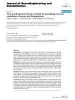
Figure 3 depicts the transfer function power spectrum (|W
(f)|
2
) for
τ
= 200, 400 and 800 ms. The figure clearly dem-
onstrates that as the length of the analysis window
decreases, the bandwidth of the filter increases. Therefore
the only information that can be ascertained with shorter
windows is that the frequency of the common modulating
input lies somewhere within the frequency range specified
by the window. Longer windows result in a better correla-
tion with coherence values at lower single frequencies
(close to zero), while shorter windows lump into a single
value a weighted expression of the coherence values in the
frequency range which they span.
Experimental methods

In this section we demonstrate the relationship between
time and frequency domain based methods to estimate
the common modulating drive using empirical data. The
methods are applied to data collected during isometric
contractions of the First Dorsal Interosseous muscle at
20% of maximal effort. Two contractions where the activ-
ities of 4 and 5 MUs were identified yielded a total of 16
pairs of coactive MUs. The periods of concurrent activity
of these MU pairs ranged between 30 s to 1 minute and
were further divided into pairs of non-overlapping 10 s
intervals resulting in a total of 50 pairs of 10 s long spike
trains. Each method was applied to these spike train pairs
and the correlation between the results yielded by the two
methods were investigated as discussed below.
The time domain method was used to estimate low fre-
quency common drive according to the method described
by De Luca and colleagues [16]. Three different time
domain estimates were formed by smoothing the spike
trains using Hanning windows of length 200, 400 and
800 ms respectively. These smoothed firing rate signals
were then digitally high pass filtered with a low frequency
cut-off of 0.75 Hz using a third order Butterworth filter to
remove the mean bias discharge rates. The cross correla-
tion coefficient function of these high pass filtered records
lim ( )
()cos[ ( )]
[() ()]
/
∆→
−

0
0
12
12
12
11 2 2
2
ρτ
πττ
yy
xx
xx x x
Sf f
SfS f
 (()16
ρτ γ
yy
xx
xx xx
xx
Sf
SfS f
f
12
12
11 22
12
0
12
17()

()
[() ()]
() ( )
/
==
ˆ
()
() ()
() ()
()
ρτ
πττ
yy
xx
if df
f
f
xx
f
Wf S f e
Wf S f df
12
12
0
1
2
11
1
2
2

2
=
−
∫
ff
xx
f
f
Wf S f df
2
22
1
2
2
18
∫∫
() ()
()
wt
t
t
()
cos
()=
+


















<≤
1
2
1
2
0
0
19
π
τ
τ
elsewhere
Wf Wf Wf Wf
RRR
() () ( )=−







+++






1
4
11
2
1
4
1
20
ττ
Wf e
f
f
R
jf
()
sin
sin
()=
− 2
21

πτ
πτ
π
Journal of NeuroEngineering and Rehabilitation 2004, 1:2 />Page 7 of 12
(page number not for citation purposes)
was then obtained and the peak value of this function
within ± 50 ms of the zero time lag was recorded and
termed the time domain common drive coefficient.
The coherence analyses were performed in a similar man-
ner to the procedure of Rosenberg and colleagues [3] for
point process data. The spike trains were represented as
binary pulse trains with ones corresponding to the firing
times of the MU's and zeros comprising the remainder of
the signal. Fourier transforms of these trains were
obtained for each appropriately windowed section and
then averaged according to equation (2). However where
Rosenberg and colleagues [3] do not use overlapping or
tapered data windows, we used overlapping, tapered Han-
ning windows of 2048 ms to optimize the variance and
bias of the estimate. With any non-parametric spectral
estimation technique, there is a trade-off between the var-
iance and both the bias and resolution of the estimation.
A window size of 2048 ms, gives a frequency resolution of
0.49 Hz, which is adequate to discriminate frequencies for
our purposes. However, when analyzing 10 s of data using
2048 ms non-overlapping windows, only 5 different
Magnitude squared spectra of Hanning window filtersFigure 3
Magnitude squared spectra of Hanning window filters. Magnitude spectra of the transfer functions of Hanning window filters
for three different time constants,
τ

= 200 ms (dotted line),
τ
= 400 ms (dashed line) and
τ
= 800 ms (solid line). As the time
constant increases the bandwidth of the filter decreases and its magnitude increases.
0 2 4 6 8 10 1
2
0
1
2
3
4
5
6
7
8
x 10
−3
Frequency (Hz)
Amplitude (V)
200ms
400ms
800ms
Journal of NeuroEngineering and Rehabilitation 2004, 1:2 />Page 8 of 12
(page number not for citation purposes)
records are available and this small number of records will
increase the variance of the estimate. Furthermore rectan-
gular windows introduce an estimation bias due to the
effect of their sidelobes. These concerns may be reduced

by using the Welch periodogram method which uses
tapered windows (to reduce spectral leakage and therefore
the estimation bias) and overlapping windows (to
increase the total number of windows and hence reduce
the variance). The minimum variance for this method is
obtained using an overlap of 62.5% [27]. The frequency
corresponding to the first zero-crossing of the Hanning fil-
ter was obtained according to equation (20) and the peak
value of the coherence in the range between 0.75 Hz and
this frequency was recorded.
A linear regression between the time domain common
drive coefficients and corresponding frequency domain
peak coherence values was performed to determine
whether a linear relationship between the two indices
existed. The regression r
2
values are reported at a signifi-
cance level of p < 0.05.
Results and discussion
Figure 4a,4b,4c displays the regression between the low
frequency time domain common drive coefficients for
Hanning windows of length 200, 400 and 800 ms and
peak low frequency coherence. All regressions are signifi-
cant at p < 0.05 and the r
2
statistics are 0.56, 0.81 and 0.80
respectively. A unitary slope line is displayed in the figure
and this describes the theoretical relationship between the
two indices. These results indicate that for the larger 400
ms and 800 ms windows, the time domain method is

more closely correlated with the coherence estimate, with
the 400 ms window yielding a marginally better fit. The
data for the smaller 200 ms window exhibits a consistent
bias, with the coherence estimate larger than the time
domain common drive estimate, whilst the 400 ms and
800 ms windowed data are more evenly distributed
around the unitary slope line, indicating less bias. There
are a number of possible factors that could contribute to
the observed mismatches between the two methods.
As demonstrated in Figure 2, the cross-correlation peak
can occur at lags slightly different than zero. A time delay
or misalignment has been shown to introduce a bias into
the coherence estimate that is proportional to the delay
and coherence magnitude and inversely proportional to
the FFT epoch duration [24]. However for delays of the
order of magnitude of ± 50 ms and FFT lengths of approx-
imately 2 s, this type of bias is very small and unlikely to
account for the observed differences between the time and
frequency domain estimates.
The use of a short duration window in the time domain
method results in the inclusion of multiple frequencies in
the time domain correlation estimation according to
equation (18). The bandwidths of descending oscillatory
drives may be variable. Thus when the descending drive
occupies a narrow bandwidth and the time domain win-
dow includes a greater range of frequencies than this
bandwidth, this will bias the time domain estimate to be
lower than the peak coherence value as is the case in figure
4a. Alternatively should the drive span a broader band-
width, the time domain measure would encompass all the

correlated frequencies into a single value and would thus
be different than the value obtained from any single peak
coherence frequency. This idea is illustrated in Figure 5
where a typical coherence plot is displayed. Superimposed
on this are vertical lines representing various moving aver-
age filter cut-off frequencies. The 0.75 Hz high pass cut-off
frequency is also displayed. Thus from the figure we see
that in this case the coherence occupies a fairly broad
bandwidth from 1–5 Hz, peaking at 1.5 Hz. The cut-off
frequency of the 200 ms filter is approximately 10 Hz and
thus the time domain estimate will include coherence val-
ues at all these frequencies which would make it signifi-
cantly different from the peak coherence. The 400 ms and
800 ms windows would better correlate with the peak
coherence frequencies and the 400 ms window would
provide a better overall index encompassing the full band-
width of the drive. However, if the middle peak at 8 Hz
were stronger and actually the main peak, the wider time
windows would miss it altogether. This emphasizes the
importance of a priori knowledge in choosing the appro-
priate time windows in the time-domain based method.
Therefore in summary, the time domain measure is more
effective in quantifying a range of frequencies into a single
index and the peak coherence estimate is better at repre-
senting the coherence at any single frequency.
Coherence estimates are typically formed from data
records of around 1–5 minutes in length [4,28,29] or
from pooled coherence measures of repeated trial meas-
urements [30]. This increases the number of non-overlap-
ping windows in the calculation, thereby reducing the

variance of the coherence estimate. Non-overlapping, rec-
tangular windows are traditionally preferred due to the
clear relationship with significance levels. Overlapping,
tapered windows will allow coherence to be estimated
from shorter data segments and parametric techniques, in
particular multivariate autoregressive (MAR) methods are
suggested for the analysis of very short duration data seg-
ments [31]. When using short records of data (<5 s), the
coherence estimates are likely to be significantly biased.
However, the time domain method is more robust for
such short data lengths and would therefore be preferred
in these situations.
The time domain method uses a high pass filter to remove
the mean bias from the smoothed signals, whereas the
Journal of NeuroEngineering and Rehabilitation 2004, 1:2 />Page 9 of 12
(page number not for citation purposes)
Regression plots for low frequency common drive time versus frequency domain techniquesFigure 4
Regression plots for low frequency common drive time versus frequency domain techniques. Regression plots for low fre-
quency common drive time versus frequency domain techniques. Three different moving average Hanning windows were used
to low pass filter the time series for the time domain method. The time constants for the filters are as follows: (a)
τ
= 200 ms,
(b)
τ
= 400 ms, (c)
τ
= 800 ms. All regressions are significant at p < 0.05 and the r
2
statistics are (a) 0.56, (b) 0.81 and (c) 0.80.
The unitary slop line is indicated in the figures as a dashed line and represents the ideal mathematical relationship.

Journal of NeuroEngineering and Rehabilitation 2004, 1:2 />Page 10 of 12
(page number not for citation purposes)
frequency domain coherence method simply subtracts the
mean component of the signal prior to forming the esti-
mate. Although similar, these two methods are not iden-
tical and may further explain some of the variation
between the time and frequency domain techniques. A
further possibility is to employ a low order polynomial
detrending technique instead of high pass filtering or sub-
tracting the mean. In general, a visual examination of the
smoothed firing rate signals would indicate whether this
would be necessary.
It is straight forward to quantify any time delay using the
time domain technique. Although this is also possible
with the frequency domain technique, this delay informa-
tion is incorporated in the phase of the estimate and is
therefore 2
π
periodic and would thus yield the same result
for integer multiples of delay. For significant coherence
present over a band of frequencies, Mima and colleagues
[32] suggest a constant phase shift plus constant time
delay regression model to compute time delays from
coherence estimates. However for narrow band
Magnitude squared coherence between two motor unit spike trains recorded from the FDI muscleFigure 5
Magnitude squared coherence between two motor unit spike trains recorded from the FDI muscle. Magnitude coherence
between two motor unit spike trains recorded from the FDI muscle. The vertical dotted lines from left to right represent the
cut-off frequencies of the 0.75 high-pass filter, and the 800 ms, 400 ms and 200 ms moving average low-pass filters. The peak
coherence occurs at 1.5 Hz.
0 2 4 6 8 10

0
0.1
0.2
0.3
0.4
0.5
0.6
Frequency (Hz)
Coherence Magnitude
HP filter
800ms filter
400ms filter
200ms filter
Journal of NeuroEngineering and Rehabilitation 2004, 1:2 />Page 11 of 12
(page number not for citation purposes)
descending drives, the time domain technique provides a
clearer estimate of any time delay.
It should be noted that the time domain technique may
be generalized to cover any arbitrary frequency. This
would necessitate bandpass filtering the signals to the
frequency range of interest, removing the mean trends
and then evaluating the cross-correlation function.
Although this requires a priori knowledge of the drive
bandwidth, this method would then be able to provide a
single index to quantify a particular bandwidth.
Conclusions
Two separate bodies of literature offer techniques to esti-
mate band limited common oscillatory input to motor
neurons. These techniques are based in either the time or
in the frequency domain. Indices derived from both meas-

urement techniques are well correlated with each other
and in the theoretical limit, the techniques are shown to
be mathematically equivalent. However, for practical pur-
poses there are a number of minor discrepancies which
may favour the use of one particular method for a given
application.
The time domain method offers greater resolution in time
(the latency of the correlations are easily revealed) at the
expense of the requirement of a priori knowledge of the
bandwidth of the common modulating drive. On the
other hand the frequency domain technique reveals infor-
mation regarding the frequency distribution of the com-
mon modulating drives but it is more difficult to obtain
accurate estimates of the coherence with short signal
lengths as well as of the exact delay.
Time domain methods of estimation are preferred for
short data segments and are well suited to quantifying the
strength of a broad band drive into a single index. This
proves useful in quantitative, comparitive analyses of the
common behavior of MUs such as statistical tests that
investigate the effects of aging or disease. Frequency
domain measures tend to be more encompassing as they
provide a complete description of all common oscillatory
inputs. This facilitates qualitative analysis of distribution
of coherence across frequencies and hence leads to a bet-
ter understanding of the nature of the common inputs.
They are well suited for estimation from large data seg-
ments, that may be assumed to be stationary, and are bet-
ter able to quantify narrow ranges of descending inputs
into a single index. Thus the selection of one technique

over another should be dictated by the nature of the phys-
iological question to be addressed.
Acknowledgements
The authors gratefully acknowledge the financial support of the Falk Medi-
cal Research Trust.
References
1. Brown P: Cortical drives to human muscle: the Piper and
related rhythms. Prog Neurobiol 2000, 60:97-108.
2. Grosse P, Cassidy MJ, Brown P: EEG-EMG, MEGEMG and EMG-
EMG frequency analysis: physiological principles and clinical
applications. Clin Neurophysiol 2002, 113:1523-1531.
3. Rosenberg JR, Amjad AM, Breeze P, Brillinger DR, Halliday DM: The
Fourier approach to the identification of functional coupling
between neuronal spike trains. Prog Biophys Mol Biol 1989,
53:1-31.
4. Farmer SF, Bremner FD, Halliday DM, Rosenberg JR, Stephens JA:
The frequency content of common synaptic inputs to
motoneurones studied during voluntary isometric contrac-
tion in man. J Physiol 1993, 470:127-155.
5. Conway BA, Halliday DM, Farmer SF, Shahani U, Maas P, Weir AI,
Rosenberg JR: Synchronization between motor cortex and spi-
nal motoneuronal pool during the performance of a main-
tained motor task in man. J Physiol 1995, 489:917-924.
6. Salenius S, Portin K, Kajola M, Salmelin R, Hari R: Cortical control
of human motoneuron firing during isometric contraction. J
Neurophysiol 1997, 77:3401-3405.
7. Halliday DM, Conway BA, Farmer SF, Rosenberg JR: Using electro-
encephalography to study functional coupling between cor-
tical activity and electromyograms during voluntary
contractions in humans. Neurosci Lett 1998, 241:5-8.

8. Mima T, Hallett M: Corticomuscular coherence: a review. J Clin
Neurophysiol 1999, 16:501-511.
9. McAuley JH, Marsden CD: Physiological and pathological trem-
ors and rhythmic central motor control. Brain 2000,
123:1545-1567.
10. Semmler JG, Kornatz KW, Enoka RM: Motor-unit coherence dur-
ing isometric contractions is greater in a hand muscle of
older adults. J Neurophysiol 2003, 90:1346-1349.
11. Brown P, Marsden J, Defebvre L, Cassim F, Mazzone P, Oliviero A,
Altibrandi MG, Di Lazzaro V, Limousin-Dowsey P, Fraix V, Odin P,
Pollak P: Intermuscular coherence in Parkinson's disease:
relationship to bradykinesia. Neuroreport 2001, 12:2577-2581.
12. Salenius S, Avikainen S, Kaakkola S, Hari R, Brown P: Defective cor-
tical drive to muscle in Parkinson's disease and its improve-
ment with levodopa. Brain 2002, 125:491-500.
13. Farmer SF, Sheean GL, Mayston MJ, Rothwell JC, Marsden CD, Con-
way BA, Halliday DM, Rosenberg JR, Stephens JA: Abnormal motor
unit synchronization of antagonist muscles underlies patho-
logical co-contraction in upper limb dystonia. Brain 1998,
121:801-814.
14. Mima T, Toma K, Koshy B, Hallett M: Coherence between corti-
cal and muscular activities after subcortical stroke. Stroke
2001, 32:2597-2601.
15. Grosse P, Guerrini R, Parmeggiani L, Bonanni P, Pogosyan A, Brown
P: Abnormal corticomuscular and intermuscular coupling in
high-frequency rhythmic myoclonus. Brain 2003, 126:326-342.
16. De Luca CJ, LeFever RS, McCue MP, Xenakis AP: Control scheme
governing concurrently active human motor units during
voluntary contractions. J Physiol 1982, 329:129-142.
17. Kamen G, Greenstein SS, De Luca CJ: Lateral dominance and

motor unit firing behavior. Brain Res 1992, 576:165-167.
18. Semmler JG, Nordstrom MA: Influence of handedness on motor
unit discharge properties and force tremor. Exp RBraines 1995,
104:115-125.
19. Adam A, De Luca CJ, Erim Z: Hand dominance and motor unit
firing behavior. J Neurophysiol 1998, 80:1373-1382.
20. Garland SJ, Miles TS: Control of motor units in human ffexor
digitorum profundus under different proprioceptive
conditions. J Physiol 1997, 502:693-701.
21. Semmler JG, Nordstrom MA, Wallace CJ: Relationship between
motor unit short-term synchronization and common drive
in human first dorsal interosseous muscle. Brain Res 1997,
767:314-320.
22. Patten C, Kamen G: Adaptations in motor unit discharge activ-
ity with force control training in young and older human
adults. Eur J Appl Physiol 2000, 83:128-143.
23. Erim Z, Beg MF, Burke DT, de Luca CJ: Effects of aging on motor-
unit control properties. J Neurophysiol 1999, 82:2081-2091.
24. Carter GC: Coherence and time delay estimation. Proc IEEE
1987, 75:236-255.
Publish with BioMed Central and every
scientist can read your work free of charge
"BioMed Central will be the most significant development for
disseminating the results of biomedical research in our lifetime."
Sir Paul Nurse, Cancer Research UK
Your research papers will be:
available free of charge to the entire biomedical community
peer reviewed and published immediately upon acceptance
cited in PubMed and archived on PubMed Central
yours — you keep the copyright

Submit your manuscript here:
/>BioMedcentral
Journal of NeuroEngineering and Rehabilitation 2004, 1:2 />Page 12 of 12
(page number not for citation purposes)
25. Gardner WA: A unifying view of coherence in signal
processing. Signal Processing 1992, 29:113-140.
26. De Luca CJ, Erim Z: Common drive of motor units in regula-
tion of muscle force. Trends Neurosci 1994, 17:299-305.
27. Marple SL: Digital spectral analysis with applications. Engle-
wood Cliffs, NJ: Prentice Hall; 1987.
28. Kristeva-Feige R, Fritsch C, Timmer J, Lucking CH: Effects of atten-
tion and precision of exerted force on beta range EEG-EMG
synchronization during a maintained motor contraction
task. Clin Neurophysiol 2002, 113:124-131.
29. Gross J, Tass PA, Salenius S, Hari R, Freund HJ, Schnitzler A: Cor-
tico-muscular synchronization during isometric muscle con-
traction in humans as revealed by
magnetoencephalography. J Physiol 2000, 527:623-631.
30. Amjad AM, Halliday DM, Rosenberg JR, Conway BA: An extended
difference of coherence test for comparing and combining
several independent coherence estimates: theory and appli-
cation to the study of motor units and physiological tremor.
J Neurosci Methods 1997, 73:69-79.
31. Cassidy MJ, Brown P: Hidden Markov based autoregressive
analysis of stationary and non-stationary electrophysiologi-
cal signals for functional coupling studies. J Neurosci Methods
2002, 116:35-53.
32. Mima T, Hallett M: Electroencephalographic analysis of cor-
tico-muscular coherence: reference effect, volume conduc-
tion and generator mechanism. Clin Neurophysiol 1999,

110:1892-1899.