Báo cáo hóa học: " Neural-Network-Based Time-Delay Estimation Samir Shaltaf" docx
Bạn đang xem bản rút gọn của tài liệu. Xem và tải ngay bản đầy đủ của tài liệu tại đây (582.47 KB, 8 trang )
EURASIP Journal on Applied Signal Processing 2004:3, 378–385
c
2004 Hindawi Publishing Corporation
Neural-Network-Based Time-Delay Estimation
Samir Shaltaf
Department of Electronic Engineering, Princess Sumaya University for Technology, P.O. Box 1438,
Al-Jubaiha 11941, Amman, Jordan
Email:
Received 4 May 2003; Revised 13 August 2003; Recommended for Publication by John Sorensen
A novel approach for estimating constant time delay through the use of neural networks (NN) is introduced. A desired reference
signal and a delayed, damped, and noisy replica of it are both filtered by a fourth-order digital infinite impulse response (IIR) filter.
The filtered signals are normalized with respect to the highest values they achieve and then applied as input for an NN system. The
output of the NN is the estimated time delay. The network is first trained with one thousand training data set in which each data set
corresponds to a randomly chosen constant time delay. The estimated time delay obtained by the NN is an accurate estimate of the
exact time-delay values. Even in the case of noisy data, the estimation error obtained was a fraction of the sampling time interval.
The delay estimates obtained by the NN are comparable to the estimated delay values obtained by the cross-correlation technique.
The main advantage of using this technique is that accurate estimation of time delay results from performing one pass of the
filtered and normalized data through the NN. This estimation process is fast when compared to the classical techniques utilized
for time-delay estimation. Classical techniques rely on generating the computationally demanding cross-correlation function of
the two signals. Then a peak detector algorithm is utilized to find the time at which the peak occurs.
Keywords and phrases: Neural networks, time-delay estimation.
1. INTRODUCTION
Time-delay estimation problem has received considerable at-
tention because of its diverse applications. Some of its appli-
cations exist in the areas of radar, sonar, seismology, commu-
nication systems, and biomedicine [1].
In active source location applications, a continuous ref-
erence signal s(t) is transmitted and a noisy, damped, and de-
layed replica of it is received. The following model represents
the received waveform:
r(t) = αs(t − d)+w(t), (1)
where r(t) is the received signal that consists of the reference
signal s(t) after being damped by an unknown attenuation
factor α, and delayed by an unknown constant value d,and
distorted by additive white Gaussian noise w(t).
A generalized cross-correlation method has been used for
the estimation of fixed time delay in which the delay esti-
mate is obtained by the location of the peak of the cross-
correlation between the two filtered input signals [2, 3]. Es-
timation of time delay is considered in [4, 5], where the least
mean square (LMS) adaptive filter is used to correlate the
two input data. The resulting delay estimate is the location
at which the filter obtains its peak value. To obtain the non-
integer value of the delay, peak estimation that involves inter-
polation is used. Etter and Stearns have used gradient search
to adapt the delay estimate by minimizing a mean square er-
ror, which is a function of the difference between the signal
and its delayed version [6]. Also, So et al. minimized a mean
square error function of the delay, where the interpolating
sinc function was explicitly parameterized in terms of the
delay estimate [7]. The average magnitude difference func-
tion (AMDF) was also utilized for the determination of the
correlation peak [8]. In [8], During has shown that recur-
sive algorithms produce better time-delay estimate than non-
recursive algorithms. Conventional prefiltering of incoming
signals used in [2] was replaced by filtering one of the in-
coming sig nals using wavelet transform [9]. Chan et al. in
[9] has used the conventional peak detection of the cross-
correlation for estimating the delay. Chan et al. reported
that their proposed algorithm outperforms the direct cross-
correlation method for constant time-delay estimation. In
[10], Wang et al. has developed a neural network (NN) sys-
tem that solves a set of unconstrained linear equations using
L
1
-norm that optimizes the least absolute deviation prob-
lem. The time-delay estimation problem is converted to a
set of linear algebraic equations through the use of higher-
order cumulants. The unknown set of coefficients represent
the parameters of a finite impulse response filter. The pa-
rameter index at which the highest parameter value occurs
represents the estimated time delay. The algorithm proposed
by Wang et al. is capable of producing delay estimates; this
Neural-Networks-Based Time-Delay Estimation 379
algorithm produces only a multiple integer of sampling inter-
val and does not deal with the case of fractional time delay.
Also, the Wang et al. algorithm has utilized the high-order
spectr a, which requires heavy computational power.
In this paper, direct estimation of constant time delay is
accomplished through the use of NN. The NN has proven
to be powerful in solving problems that entail classification,
approximation of nonlinear relations, interpolation, and sys-
tem identification. It has found its way into many applica-
tions in speech and image processing, nonlinear control, and
many other areas.
In this paper, the capability of generalization and inter-
polation of the NN is employed in the area of time-delay es-
timation. The NN is trained with many different sets of data
that consist of the reference signal and its damped, delayed,
and noisy replica. A fourth-order type II Chebyshev band-
pass digital filter is used to filter the two signals. The filtered
signals are normalized with respect to the highest values the y
achieve before they are applied to the NN input. The noise-
free reference signal is filtered to make it experience the same
transient effect and phase shift the filtered delayed noisy sig-
nal has experienced.
The rest of this paper is organized as follows. Section 2
presents the details of the proposed technique of using the
NN for the estimation of constant time delay. Section 3
presents the simulation results of the proposed technique.
The conclusion is presented in Section 4.
2. TIME-DELAY ESTIMATION ALGORITHM
The reference signal s(t) is assumed to be a sinusoidal signal
with frequency Ω
o
rad/s, and sampled with a sampling period
T seconds. The resulting discrete reference signal is
s(n) = sin
ω
o
n
,(2)
where ω
o
= Ω
o
T is the frequency of the sampled reference
signal. Assuming the received signal in (1)hasbeenfiltered
by an antialiasing filter and then sampled, then its discrete
form is
r(n) = αs(n − D)+w(n), (3)
where s(n − D) is the delayed reference signal, D is an un-
known constant delay measured in samples and related to the
time delay d by the relation D = d/T, α is an unknown damp-
ing factor, and w(n) is zero-mean white Gaussian noise with
variance σ
2
w
. Finite length data windows are obtained from
the sampled reference signal and the damped, noisy, and de-
layed signal with a length of N samples.
Let s = [s(0), s(1), , s(N − 1)] and r = [r(0), r(1),
, r(N − 1)] be the vector forms of the two data windows
representing the reference and the received signals, respec-
tively. Since the received signal is noisy, it is best that it gets
filtered in order to obtain better estimate for the unknown
time delay.
A fourth-order type II Chebyshev bandpass digital filter
was used to filter the two signals. The filter was designed to
have a narrow pass bandwidth equal to 0.02 radian with 2 dB
attenuation for the two pass frequencies and a stop band
bandwidth of 0.32 radian with a 40 dB attenuation for the
stop frequencies. The center frequency ω
c
of the bandpass
filter was set equal to the reference signal frequency ω
o
,and
was set to be exactly equal to the geometric mean of the pass
and stop frequencies. The resulting bandpass digital filter or-
der that satisfies the above conditions was found to be 4.
The strict narrow bandwidth condition resulted in a band-
pass filter that was capable of reducing the input noise power
to about 1.6% of its value at the filter output. This means a
noise reduction factor equal to 62.5, which implies a signal-
to-noise ratio improvement by 18 dB. This improvement on
the signal-to-noise ratio results in improving the accuracy of
the time-delay estimates.
Let the filter frequency response be H(ω) and assume that
the filter input is a white Gaussian noise w(n) having zero
mean and variance σ
2
w
. Let the filter output be y(n). The out-
put signal y(n) will then be a zero-mean colored Gaussian
noise with variance σ
2
y
,where
σ
2
y
=
1
2π
π
−π
σ
2
w
H(ω)
2
dω. (4)
The frequency response H(ω) of the bandpass filter was ob-
tained through the Matlab environment. The white Gaussian
noise w(n) was assumed to have a unit variance σ
2
w
= 1. The
output signal variance σ
2
y
was calculated through the Matlab
to have a value of 0.016.
The bandpass filter is used to filter the received noisy sig-
nal and improve the signal-to-noise ratio which is a needed
step before applying the signal to the NN. The reference sig-
nal s(n) is also filtered by the same filter to make it experience
the same effect the received filtered signal has experienced.
Thetwosignalsarenowinperfectmatchwitheachotherex-
cept for the unknown constant time-delay value D and the
damping factor α. To eliminate the effect of the presence of
the damping factor α, the two filtered signals are normalized
with respect to the highest values they achieve. Normalizing
the filtered signals is used to prevent the NN from being af-
fected by the different amplitude variations of the signals due
to the different and unknown damping factors. The signal-
to-noise ratio which is a very important determining factor
of the accuracy of the time-delay estimate is not affected by
the normalization step. By applying the filtered and normal-
ized signals to the NN, the NN should then be capable of pro-
ducing accurate time-delay estimates. If the received noisy
signals were u sed instead, the NN would produce time-delay
estimateswhicharefarfrombeingaccurate.
Let h(n) be the impulse response of the filter and apply
the signals s(n)andr(n) as inputs to the filter; the corre-
sponding outputs are
s
f
(n) =
n
k=0
h(k)s(n − k), n = 0, , N − 1,
r
f
(n) =
n
k=0
h(k)r(n − k), n = 0, , N − 1,
(5)
380 EURASIP Journal on Applied Signal Processing
Table 1: Parallel input mode (exact delay d = 0.153 second, damping factor α = 1).
Neural Network
Noise SD = 0.1 Noise SD = 0.3 Noise SD = 0.5
E[d]SDEEE[d]SDEEE[d]SDEE
1 P-128-5-1 0.1599 0.0023 0.1497 0.0069 0.1506 0.0118
2 P-128-10-1 0.1545 0.0025 0.1545 0.0074 0.1539 0.0143
3 P-128-20-1 0.1533 0.0026 0.1550 0.0103 0.1578 0.0226
4 P-128-10-1-1 0.1511 0.0031 0.1521 0.0089 0.1513 0.0146
5 P-128-10-5-1 0.1530 0.0020 0.1529 0.0065 0.1526 0.0115
6 P-128-10-10-1 0.1524 0.0028 0.1527 0.0082 0.1524 0.0205
7 128-Cross-1 0.1525 0.0020 0.1524 0.0063 0.1525 0.0097
8 128-Cross-2 0.1562 0.0023 0.1564 0.0071 0.1558 0.0114
9 P-256-5-1 0.1482 0.0022 0.1482 0.0069 0.1501 0.0114
10 P-256-10-1 0.1513 0.0030 0.1534 0.0091 0.1555 0.0134
11 P-256-20-1 0.1535 0.0031 0.1529 0.0097 0.1549 0.0168
12 P-256-10-1-1 0.1564 0.0020 0.1573 0.0059 0.1576 0.0099
13 P-256-10-5-1 0.1555 0.0018 0.1553 0.0056 0.1537 0.0222
14 P-256-10-10-1 0.1503 0.0009 0.1506 0.0025 0.1501 0.0118
15 256-Cross-1 0.1528 0.0015 0.1527 0.0044 0.1532 0.0073
16 256-Cross-2 0.1535 0.0017 0.1534 0.0051 0.1534 0.0085
where only the first N samples of both of the filtered signals
are obtained. The filtered signals are then normalized w ith
respect to the highest values they achieve. The two filtered
signals carry a transient effect due to the filtering step by the
narrow bandpass filter. The transient effect present on the
two filtered signals introduces no problem to the NN since
the constant time delay is still present between the two fi l-
tered signals and is not changed through the filtering step.
The two filtered and normalized signals are applied in
three different ways to the NN. In the first method, called
the parallel input form, the two signals are concatenated to-
gether to form the input vector. The resulting input vector
is twice as large as either of the filtered signals. In the sec-
ond method, called the difference input form, the difference
between the two signals is applied to another NN system.
The third method, called the single input form, uses only
the filtered and normalized received signal as the NN input.
The reference signal is not used as a part of the NN input.
The motivation behind this method stems from the fact that
the time delay is imbedded into the received signal. The dif-
ference and the single input forms use input vectors with
lengths equal to half of the input vector length for the par-
allel input form, hence resulting in a large reduction in the
NN size.
In the training phase, about one thousand data set with
the corresponding time-delay values were introduced a s
training examples to the NN. For each training example, uni-
form random generator generated the time-delay value ran-
domly. The time delay assume real values ranging uniformly
from 0.0 to 0.5 seconds. The sampling interval was assumed
to ha ve a value of T = 0.05 seconds. This results in time-
delay values in the range of 0 to 10 sampling intervals. The
damping factor α was generated by a uniform random gen-
erator to have any value in the range of 0.25 to 1. The distort-
ing noise added to the delayed signal is zero-mean Gaussian
with standard deviation values chosen randomly by a uni-
form random generator to have any value between 0.0 and
0.5. This step is performed so that the NN is trained with
data sets that experienced different levels of noise.
The neural network systems used in this paper were feed-
forward networks. Two-layer and three-layer networks were
used. Hyperbolic tangent nonlinearity was used for the hid-
den layer neurons, while linear transfer function was used
for the output neuron. Improved version of the backprop-
agation training algorithm was used for training the net-
work. It is called resilient backpropagation [11]. Riedmiller
and Braun in [11] had noticed that the nonlinear transfer
functions, the hyperbolic tangent and the log sigmoid, of the
neurons have very small gradient values for large input val-
ues. The small gradient values result in slow convergence for
the NN in the training phase because the backpropagation is
gradient-based learning algorithm. In order to overcome this
problem, the sign of the gradient was used instead of its small
value to update the NN parameters. This resulted in a major
improvement on the speed of convergence of the NN.
Two-layer and three-layer NNs were used for the three
input forms. Tab le 1 presents the NN which use the parallel
input form, Table 2 presents the NN which use the difference
input form, and Tabl e 3 presents the NN which use the sin-
gle input form. The three-layer NNs representation used for
the parallel input form is denoted by P-N-M-K-1 notation,
where P denotes that the para llel input form is being used,
Neural-Networks-Based Time-Delay Estimation 381
Table 2: Difference input mode (exact delay d = 0.153 second, damping factor α = 1).
Neural Network
Noise SD = 0.1 Noise SD = 0.3 Noise SD = 0.5
E[d]SDEEE[d]SDEEE[d]SDEE
1 D-128-5-1 0.1533 0.0021 0.1528 0.0065 0.1519 0.0116
2 D-128-10-1 0.1525 0.0027 0.1523 0.0084 0.1523 0.0145
3 D-128-20-1 0.1515 0.0024 0.1514 0.0073 0.1516 0.0127
4 D-128-10-1 0.1546 0.0024 0.1531 0.0077 0.1509 0.0139
5 D-128-10-5-1 0.1534 0.0020 0.1530 0.0063 0.1531 0.0108
6 D-128-10-10-1 0.1537 0.0026 0.1535 0.0077 0.1541 0.0134
7 128-Cross-1 0.1525 0.0020 0.1524 0.0063 0.1525 0.0097
8 128-Cross-2 0.1562 0.0023 0.1564 0.0071 0.1558 0.0114
9 D-256-5-1 0.1543 0.0017 0.1545 0.0047 0.1548 0.0084
10 D-256-10-1 0.1534 0.0020 0.1529 0.0063 0.1524 0.0110
11 D-256-20-1 0.1509 0.0021 0.1555 0.0073 0.1616 0.0134
12 D-256-10-1-1 0.1570 0.0040 0.1569 0.0117 0.1563 0.0205
13 D-256-10-5-1 0.1523 0.0019 0.1525 0.0055 0.1530 0.0103
14 D-256-10-10-1 0.1533 0.0019 0.1534 0.0067 0.1541 0.0109
15 256-Cross-1 0.1528 0.0015 0.1527 0.0044 0.1532 0.0073
16 256-Cross-2 0.1535 0.0017 0.1534 0.0051 0.1534 0.0085
Table 3: Single input mode (exact delay d = 0.153 second, damping factor α = 1).
Neural Network
Noise SD = 0.1 Noise SD = 0.3 Noise SD = 0.5
E[d]SDEEE[d]SDEEE[d]SDEE
1 S-128-5-1 0.1576 0.0024 0.1582 0.0069 0.1578 0.0117
2 S-128-10-1 0.1524 0.0029 0.1528 0.0080 0.1539 0.0131
3 S-128-20-1 0.1529 0.0024 0.1523 0.0074 0.1514 0.0125
4 S-128-10-1-1 0.1542 0.0023 0.1536 0.0072 0.1521 0.0120
5 S-128-10-5-1 0.1506 0.0027 0.1520 0.0079 0.1524 0.0130
6 S-128-10-10-1 0.1503 0.0023 0.1508 0.0069 0.1511 0.0130
7 128-Cross-1 0.1525 0.0020 0.1524 0.0063 0.1525 0.0097
8 128-Cross-2 0.1562 0.0023 0.1564 0.0071 0.1558 0.0114
9 S-256-5-1 0.1498 0.0042 0.1503 0.0126 0.1529 0.0198
10 S-256-10-1 0.1519 0.0032 0.1543 0.0093 0.1576 0.0144
11 S-256-20-1 0.1535 0.0018 0.1537 0.0057 0.1531 0.0098
12 S-256-10-1-1 0.1527 0.0018 0.1526 0.0058 0.1519 0.0090
13 S-256-10-5-1 0.1525 0.0020 0.1521 0.0056 0.1521 0.0094
14 S-256-10-10-1 0.1528 0.0020 0.1524 0.0057 0.1523 0.0105
15 256-Cross-1 0.1528 0.0015 0.1527 0.0044 0.1532 0.0073
16 256-Cross-2 0.1535 0.0017 0.1534 0.0051 0.1538 0.0085
N represents the length of each of the two input vectors, M
represents the number of neurons in the first hidden layer, K
represents the number of neurons in the second hidden layer,
and the last character is the numeral 1 which is equal to the
length of the output layer. The output layer is a single output
neuron which outputs the estimated time delay. Similarly, the
two-layer network P-N-M-1 represents a parallel input form
structure with each of the two input vectors having a length
equal to N, the single hidden layer consists of M neurons,
and the output consists of a single neuron. Similar notation
382 EURASIP Journal on Applied Signal Processing
is used for the difference input form where P is replaced by
D. Also, the single input form networks start with the letter S.
Tables 2 and 3 show different representations of a two and a
three-layer networks using difference and single input forms,
respectively.
2.1. Parallel input form
The two filtered and normalized signals s
f
= [s
f
(0), s
f
(1), ,
s
f
(N − 1)] and r
f
= [r
f
(0), r
f
(1), , r
f
(N − 1)] are concate-
nated into one vector x = [s
f
, r
f
]. The resulting vector x
is twice the length of any of the two filtered signals. Vector
x is applied to the NN as the training input, and the corre-
sponding time delay d as the desired delay output in seconds.
Since the length of each of the filtered signals is N, the NN
for the parallel input form has 2N input nodes for its input
layer.
The network represented by the P-256-10-5-1 notation
found in Table 1 represents a three-layer parallel input form
structure where the length of each of the two inputs is 256.
The total number of inputs for this NN is 512. The first hid-
den layer consists of 10 neurons and the second hidden layer
consists of 5 neurons. The output layer is a single output neu-
ron. Also, the two-layer network P-128-20-1 in Ta ble 1 rep-
resents a parallel input form structure with a total number of
256 inputs, 20 neurons for the single hidden layer, and one
output neuron.
2.2. Difference input form
The difference between the two filtered signals, y = s
f
− r
f
,
is obtained and then applied to the input of the NN. The
length of this vector is N. By using the difference input form
structure, the input layer of the NN is reduced by a factor
of two when compared to the parallel input form structure.
This results in an appreciable reduction in the NN size. The
three-layer difference input form with 128 input nodes, 10
neurons for the first hidden layer, 5 neurons for the second
hidden layer, and one output neuron, is denoted by D-128-
10-5-1 as seen in Tabl e 2.
2.3. Single input form
In this method, only the filtered and normalized signal r
f
is
applied to the NN. The reason behind using r
f
is that the
time delay is embedded into the signal r
f
. The three-layer
single input form with 128 input nodes, 10 neurons for the
first hidden layer, 5 neurons for the second hidden layer, and
one output neuron, is denoted by S-128-10-5-1 as seen in
Table 3. All of the three input form s tructures are presented
in Figure 1.
3. SIMULATION RESULTS
The simulation section consists of four sections. Sections 3.1,
3.2,and3.3 test the three different input forms under differ-
ent input lengths and different noise levels. In those sections,
the damping ratio is set equal to one. Section 3.4 tests the best
performing structures obtained in the first three sections un-
der different noise levels and different damping ratios.
Input
vector
Input
layer
Hidden
layer
Output
layer
Output
delay
x = [s
f
, r
f
]
d
(a)
y = [s
f
− r
f
]
d
(b)
y = [s
f
]
d
(c)
Figure 1: NNs with three input mode schemes: (a) parallel input
mode with 2N inputs, ( b) difference input mode with N inputs,
and ( c) single input mode with N inputs.
The NN were trained with the filtered and normalized
signals r
f
and s
f
. The delayed signal was additively distorted
with a zero-mean white Gaussian noise. The standard devi-
ation of the Gaussian noise was randomly generated in the
range of 0 to 0.5, which corresponds to noise variance of
0to0.25. The damping factor was randomly generated to
have any value in the range of 0.25 to 1. About 1000 data
sets were used in the training phase. The signals were delayed
Neural-Networks-Based Time-Delay Estimation 383
by randomly selected time-delay values. A uniform random
number generator generated the time-delay values that were
used in the training phase. The time-delay values were cho-
sentohaveanyvaluebetween0and0.5 second, which cor-
responds to 0 to 10 sampling intervals. The frequency of the
reference sinusoidal signal was chosen equal to 6 rad/sec and
sampled with a sampling period of T = 0.05 second, hence
resulting in discrete reference signal s( n) = sin(0.3n).
In the testing phase, 1000 data sets were introduced to the
NN input. These data sets were distorted with three different
noise levels. These noise levels had standard deviation values
σ = 0.1, 0.3, and 0.5. Two different record lengths were used,
N = 128 and N = 256, for each noise level. Also two-layer
and three-layer NNs were used. The time-delay value used
for all of the testing data sets was chosen to be 0.153 sec-
ond which corresponds to 3.06 sampling intervals. The NN
was tested to estimate the time delay under different damp-
ing factor values. In Sections 3.1, 3.2,and3.3, the damping
factor value was set equal to one. While in Section 3.4, the
damping factor was set equal to 0.25, 0.5, and 0.75.
For comparison reasons, delay estimates were obtained
by the classical cross-correlation technique. The cross-
correlation was applied to the noise-free reference signal s(n)
and the delayed, damped, and noisy signal r(n). This estima-
tionprocessisdenotedbyN-Cross-1, where N equals 128 or
256 samples. Also, the estimation of time delay was obtained
through the cross correlation between the filtered noise-free
signal s
f
and the filtered delayed noisy signal r
f
. This estima-
tionprocessisdenotedbyN-Cross-2. The N-Cross-1 estima-
tion process produced more accurate results than N-Cross-2
when large damping factors were used. The delay estimates
obtained by the NN were accurate but the cross- correlation
estimates performed slightly better than the NN systems. In
one case, the NN standard deviation estimation error (SDEE)
was less than that obtained by the cross-correlation. It is ob-
served that when the signal is highly attenuated, it results in
time-delay estimate with large SDEE. This is explained by the
statistical estimation principle which states that estimation
error gets larger when signals with lower signal-to-noise ra-
tios are used [12].
3.1. Parallel input form
The reference signal s
f
, the filtered and delayed noisy signal
r
f
, and time delay d were used in the training phase of the
NN. The input vector for the NN was x = [s
f
, r
f
]. It has a
length that is twice the length of any of the two signal vec-
tors. Table 1 presents the ensemble average of the estimated
time-delay values and the corresponding SDEE obtained by
the NN and the cross-correlation techniques. The number of
the testing data sets used was equal to one thousand. Each of
these data sets was corrupted with noise having standard de-
viation values σ = 0.1, 0.3, and 0.5. The damping factor used
in all of the testing data sets was set equal to one.
It is observed from the results presented in Tabl e 1 that
the SDEE is low when low noise levels are used. Rows 1 to
6inTable 1 correspond to data lengths of 128 samples for
each of the filtered signals, w here rows 1, 2, and 3 correspond
to the two-layer NN and rows 4, 5, and 6 correspond to the
400
200
0
0.10.11 0.12 0.13 0.14 0.15 0.16 0.17 0.18 0.19 0.2
Time delay (s)
Standard deviation = 0.1
No. of
delay estimates
400
200
0
0.10.11 0.12 0.13 0.14 0.15 0.16 0.17 0.18 0 .19 0.2
Time delay (s)
Standard deviation = 0.3
No. of
delay estimates
400
200
0
0.10.11 0.12 0.13 0.14 0.15 0.16 0.17 0.18 0 .19 0.2
Time delay (s)
Standard deviation = 0.5
No. of
delay estimates
Figure 2: Histogram for the delay estimate of a delay value of 0.153
second using three different noise levels with standard deviations of
0.1, 0.3, and 0.5. The NN used is the difference input mode D256-
10-10-1 structure.
three-layer NN. The next two rows, 7 and 8 correspond, to
the 128-Cross-1 and 128-Cross-2 estimation results, respec-
tively. Also, rows 9 to 14 correspond to the two-layer and the
three-layer NNs using 256 samples. Rows 15 and 16 corre-
spond to the 256-Cross-1 and the 256-Cross-2 estimation re-
sults.
Amongst the networks using 128 samples for its inputs,
the three-layer network P-128-10-5-1 produced the most ac-
curate results in terms of the SDEE. The SDEE values are very
close to those values obtained by the 128-Cross-1 and bet-
ter than those obtained by the 128-Cross-2. The two-layer
network P-128-5-1 resulted in time-delay estimates with the
SDEE values almost equal to the 128-Cross-2 technique.
Amongst the networks using 256 samples, the P-256-10-10-
1 network produced time-delay estimates with SDDE less
than those obtained by the cross-correlation techniques for
noise levels of 0.1and0.3. For higher noise levels, the cross-
correlation techniques performed better.
3.2. Difference input form
The difference signal, y = s
f
− r
f
, was applied to the NN. The
damping factor used in all of the testing data was set equal to
one. The estimation results are presented in Ta ble 2 . The best
performing network amongst those with input record length
of 128 samples is the three-layer network D-128-10-5-1. It
384 EURASIP Journal on Applied Signal Processing
Table 4: Best performing networks (exact delay d = 0.153 second, damping factor α = 0.25, 0.5, and 0.75).
Neural Network
Noise SD = 0.1 Noise SD = 0.3 Noise SD = 0.5
E[d] SDEE E[d] SDEE E[d] SDEE
P-128-10-5-1 0.1526 0.0116 0.1571 0.0283 0.1598 0.0527
D-128-10-5-1 0.1522 0.0100 0.1477 0.0335 0.1339 0.0770
S-128-5-1 0.1532 0.0093 0.1561 0.0329 0.1597 0.0537
128-Cross-1 0.1532 0.0084 0.1416 0.1095 0.1034 0.5506
128-Cross-2 0.1562 0.0092 0.1560 0.0295 0.1527 0.0843
Neural Network
Noise SD = 0.1 Noise SD = 0.3 Noise SD = 0.5
E[d] SDEE E[d] SDEE E[d] SDEE
P-128-10-5-1 0.1524 0.0060 0.1543 0.0166 0.1549 0.0253
D-128-10-5-1 0.1527 0.0051 0.1519 0.0149 0.1500 0.0267
S-128-5-1 0.1531 0.0043 0.1532 0.0148 0.1542 0.0259
128-Cross-1 0.1523 0.0041 0.1525 0.0122 0.1484 0.0702
128-Cross-2 0.1562 0.0045 0.1563 0.0136 0.1558 0.0233
Neural Network
Noise SD = 0.1 Noise SD = 0.3 Noise SD = 0.5
E[d] SDEE E[d] SDEE E[d] SDEE
P-128-10-5-1 0.1522 0.0039 0.1521 0.0113 0.1546 0.0181
D-128-10-5-1 0.1529 0.0031 0.1529 0.0103 0.1511 0.0169
S-128-5-1 0.1532 0.0028 0.1532 0.0091 0.1539 0.0163
128-Cross-1 0.1523 0.0028 0.1526 0.0081 0.1522 0.0140
128-Cross-2 0.1562 0.0032 0.1561 0.0092 0.1559 0.0153
produced the least SDEE. Also, the two-layer network D-128-
5-1 produced delay estimate with SDEE which are very close
to that obtained by the D-128-10-5-1 network. Amongst the
networks with inputs of 256 samples, the D-256-5-1 network
performed the best amongst its class.
3.3. Single input form
For this input form, only the filtered, noisy, and delayed sig-
nal r
f
was applied to the NN. The damping factor used was
set equal to one. Among the first six NN structures with in-
put length of 128, the S-128-5-1 resulted in the least SDEE.
The best performing NN structures amongst those with in-
puts of 256 samples are the S-256-20-1 and the S-256-10-1-1
networks.
Comparing all NN results against each other, it is ob-
served that the parallel input network performs better than
the best performing networks of the difference input mode
and the single input mode structures for record lengths of
256 samples. However, It must be noted that the parallel in-
put form network has a total number of inputs equal to twice
that of the other input forms. Therefore, a fair comparison
should actually compare, for example, the P-128-10-1 net-
work against the D-256-10-1 and the S-256-10-1 networks.
In such a case, it wil l be observed that the best performing
NN structure is the difference input form.
In Figure 2, histogram plots are shown for 1000 testing
data sets that were delayed by 0.153 second with noise levels
σ = 0.1, 0.3, and 0.5 having damping factor equal to one. The
histograms are produced for the network structure D-256-5-
1. The histograms are observed to have Gaussian distribution
centered at the time-delay estimate, which is near 0.153 sec-
ond. It is also observed that as the noise level increases, the
distribution widens which means that estimation error be-
comes larger.
3.4. Best performing networks
In this section the best performing networks in Sections 3.1,
3.2, 3.3,and3.4 are tested under noise levels of 0.1, 0.3, and
0.5, with record length of 128 samples, and damping fac-
tors of 0.25, 0.5, and 0.75. Tabl e 4 presents the simulation
results for the damping factors α = 0.25, 0.5, and 0.75, re-
spectively. The ensemble averages of the time delay and the
SDEE present in Table 4 correspond to 1000 data set for each
damping factor and noise level.
Comparing the resulting SDEE values for the three dif-
ferent input networks, it is observed that the single input
Neural-Networks-Based Time-Delay Estimation 385
network wins over the parallel and the difference input net-
works. It must be remembered that the results obtained in
Table 4 correspond to damping factors 0.25, 0.5, and 0.75. It
is also observed that when low damping values are used, the
SDEE estimation error gets higher. Simulation results present
in Table 4 for α = 0.25 show that the NN delay estimates
are more accurate than that of the 128-Cross-1 technique for
large noise levels of 0.3and0.5.
4. CONCLUSION
NNs were utilized, for the first time, in estimating constant
time delay. The NNs were trained by the filtered noisy and
delayed signal and the noise-free signal. Accurate time-delay
estimates were obtained by the NN through the testing phase.
The fast processing speed of the NN is the main advantage of
using NN for estimation of time delay. Time-delay estimates
obtained through classical techniques rely on obtaining the
cross correlation between the two signals and on perform-
ing interpolation to obtain the time-delay at which the peak
of the cross correlation exists. These two steps are compu-
tationally demanding. The NN performs those two steps in
one single pass of the data through its feedforward struc-
ture. The NN obtained accurate results and in one case pro-
duced delay estimates with smaller SDEE than that obtained
by the cross-correlation techniques. Although the results ob-
tained by the NN are very much encouraging, further re-
search is still needed on the reduction of the NN size with-
out reducing the data size. Also, it will be a major advance-
ment if NN can be made to deal with the case in which both
of the two signals are unknown. Estimating time-vary ing
delay with NN is a nother promising subject. Estimation of
time delay by NN has the potential of online implementa-
tion bases through the use VLSI. This will result in very fast
and accurate time-delay estimates that cannot be obtained
through classical techniques that demand heavy computa-
tional power.
REFERENCES
[1] G. C. Carter, Ed., “Special issue on time-delay estimation,”
IEEE Trans. Acoustics, Speech, and Signal Processing, vol. ASSP-
29, no. 3, 1981.
[2] C. H. Knapp and G. C. Carter, “The generalized correlation
method for estimation of time delay,” IEEE Trans. Acoustics,
Speech, and Signal Processing, vol. ASSP-24, no. 4, pp. 320–
327, 1976.
[3] G. C. Carter, “Coherence and time-delay estimation,” Pro-
ceedings of the IEEE, vol. 75, no. 2, pp. 236–255, 1987.
[4] P. L. Feintuch, N. J. Bershad, and F. A. Reed, “Time-delay
estimation using the LMS adaptive filter-dynamic behavior,”
IEEE Trans. Acoustics, Speech, and Signal Processing, vol. ASSP-
29, no. 3, pp. 571–576, 1981.
[5] Y.T.Chan,J.M.F.Riley,andJ.B.Plant, “Modelingoftime-
delay and its application to estimation of nonstationary de-
lays,” IEEE Trans. Acoustics, Speech, and Signal Processing, vol.
ASSP-29, no. 3, pp. 577–581, 1981.
[6] D. M. Etter and S. D. Stearns, “Adaptive estimation of time
delays in sampled data systems,” IEEE Trans. Acoustics, Speech,
and Signal Processing, vol. ASSP-29, no. 3, pp. 582–587, 1981.
[7] H. C. So, P. C. Ching, and Y. T. Chan, “A new algorithm for ex-
plicit adaptation of time delay,” IEEE Trans. Signal Processing,
vol. 42, no. 7, pp. 1816–1820, 1994.
[8] C. During, “Recursive versus nonrecursive correlation for
real-time peak detection and tracking,” IEEE Trans. Signal
Processing, vol. 45, no. 3, pp. 781–785, 1997.
[9] Y. T. Chan, H. C. So, and P. C. Ching, “Approximate max-
imum likelihood delay estimation via orthogonal wavelet
transform,” IEEE Trans. Signal Processing,vol.47,no.4,pp.
1193–1198, 1999.
[10] Z. Wang, J. Y. Cheung, Y. S. Xia, and J. D. Z. Chen, “Neu-
ral implementation of unconstrained minimum L
1
-norm
optimization—least absolute deviation model and its appli-
cation to time delay estimation,” IEEE Trans. on Circuits and
Systems II: Analog and Digital Signal Processing, vol. 47, no. 11,
2000.
[11] M. Riedmiller and H. Braun, “A direct adaptive method for
faster backpropagation learning: the RPROP algorithm,” in
Proc.IEEEInt.Conf.onNeuralNetworks, pp. 586–591, San
Francisco, Calif, USA, 1993.
[12] H. L. V. Trees, Detection, Estimation and Modulation Theory,
Part I, John Wiley & Sons, NY, USA, 1968.
Samir Shaltaf wasborninAmman,Jordan,
in 1962. He received his Ph.D. degree in
engineering, sensing, and signal processing,
in 1992 from Michigan Technological Uni-
versity, Michigan, USA. He joined Amman
University from 1992 to 1997. Since 1997,
he has been a faculty member of the Elec-
tronic Engineering Department at Princess
Sumaya University College for Technology.
His research interests are in the areas of
time-delay estimation, adaptive signal processing, genetic algo-
rithms, and control systems.