Báo cáo hóa học: " Object-Based and Semantic Image Segmentation Using MRF" docx
Bạn đang xem bản rút gọn của tài liệu. Xem và tải ngay bản đầy đủ của tài liệu tại đây (3.42 MB, 8 trang )
EURASIP Journal on Applied Signal Processing 2004:6, 833–840
c
2004 Hindawi Publishing Corporation
Object-Based and Semantic Image
Segmentation Using MRF
Feng Li
Shanghai Zhongke Mobile Communication Research Center, Shanghai Div ision, Institute of Computing Technology,
Chinese Academy of Sciences, Shanghai 201203, China
Institute for Pattern Recognition & Artificial Intelligence, State Education Commission Laboratory for Image Processing &
Intelligence Control, Huazhong University of Science and Technology, Wuhan 430074, China
Email:
Jiaxiong Peng
Institute for Pattern Recognition & Artificial Intelligence, State Education Commission Laboratory for Image Processing &
Intelligence Control, Huazhong University of Science and Technology, Wuhan 430074, China
Email:
Xiaojun Zheng
Shanghai Zhongke Mobile Communication Research Center, Shanghai Div ision, Institute of Computing Technology,
Chinese Academy of Sciences, Shanghai 201203, China
Email:
Received 6 December 2002; Rev ised 3 September 2003
The problem that the Markov random field (MRF) model captures the structural as well as the stochastic textures for remote
sensing image segmentation is considered. As the one-point clique, namely, the external field, reflects the priori knowledge of
the relative likelihood of the different region types which is often unknown, one would like to consider only two-pairwise clique
in the texture. To this end, the MRF model cannot satisfactorily capture the structural component of the texture. In order to
capture the structur al texture, in this paper, a reference image is used as the external field. This reference image is obtained by
Wold model decomposition which produces a purely random texture image and structural texture image from the original image.
The structural component depicts the periodicity and directionality characteristics of the texture, while the former describes the
stochastic. Furthermore, in order to achieve a good result of segmentation, such as i mproving smoothness of the texture edge,
the proportion between the external and internal fields should be estimated by regarding it as a parameter of the MRF model.
Due to periodicity of the structural texture, a useful by-product is that some long-range interaction is also taken into account. In
addition, in order to reduce computation, a modified version of parameter estimation method is presented. Experimental results
on remote sensing image demonstrating the performance of the algorithm are presented.
Keywords and phrases: semantic and structural segmentation, MRF, Wold model, remote sensing image.
1. INTRODUCTION
In this paper, remote sensing image segmentation based on
the Markov random field (MRF) is considered. Many ap-
proaches have used MRF as a label process (as discussed in
[1, 2, 3, 4, 5, 6, 7, 8, 9]), including the application to extract
urban areas in remote sensing images (as discussed elsewhere
in [5, 10, 11]). This is because exploiting MRF offers sev-
eral advantages over simple segmentation algorithms. First,
the segmentation for the object in a remote sensing image
depends not only on the gray level, but also on other fea-
tures such as texture, which can be viewed as realizations
from a parametric probability distribution model in the im-
age space. Second, this approach is flexible because it has a
few number of par ameters to set. Finite number of param-
eters characterizing spatial interactions of pixels is used to
describe an image region. Also, the constraint of smooth-
ness is meant to express the implicit assumption for texture
segmentation, that is, each separated region has to extend
over a significant area. Isolate labels and very small regions
are disal lowed because the texture pattern essentially can be
discerned only in a large enough area. There are two ba-
sic methods for the usage of the MRF model. First (as dis-
cussed elsewhere in [12, 13]), parameters are extracted as
834 EURASIP Journal on Applied Signal Processing
texture features, including mean, variance, potential param-
eters combined with other features, and then clustering cri-
teria are employed to classify the image. Its advantage is sim-
ple computation. Another method (as discussed elsewhere in
[1, 2, 3, 4, 5, 6, 7, 8, 9]) uses double random fields based on
Bayesian framework. The advantage of this method is that
prior information can be easily incorporated. Some high-
level prior information can be incorporated into this frame-
work, but the computation for combination optimization is
undesirable.
There are some deficiencies of the MRF model in im-
age analysis. Firstly, the hypothesis of homogeneous prop-
erty for random field does not accord with most pr actical im-
ages, leading to smoothness in the texture edge. However, if
a nonhomogeneous random field is used, which is relative to
position and orientation, there are a number of parameters
which inevitably bring s about enormous computation. Sec-
ondly, Markovian prior model is a low-level prior model. It
is short of semantic information and will lead to a condition
in which the segmented regions are often not consistent w ith
the object. Thirdly, as the single-clique potential prior infor-
mation, namely, the external field, is often unknown, the use
of only pairwise interaction in the Markovian model will lead
to a result in which it cannot accurately capture the structural
component of the texture.
These questions cause poor quality segmentation or in-
crease the computation time. As the segmentation process is
a basic step followed by other image analyses such as com-
pression and interpretation, an improved method is needed.
It is well known that a difficulty in using MRF model, in-
cluding single-clique potential, is the introduction of ap-
propriate prior information of single-pixel cliques. As dis-
cussedbyPicard[14], the authors conclude that if it were not
for competition from the internal field, the synthesized ran-
dom field would align itself perfectly with the desired exter-
nal field. They suggest that nonhomogeneous external field
can be set to the value in some reference image. But they
did not give such a reference image; in addition, they c an-
not estimate the relative strengths of the two fields. In this
study, we address and settle several issues left open there.
In addition, we apply this idea to image segmentation. We
will adopt a kind of Wold decomposition which can obtain
pure random field and structural field. The main contribu-
tion of this paper is to extract structural component as a
reference image of the external field of the MRF model. We
thus incorporate the structural component to the segmented
image.
Most natural textures can be modeled as a superposition
of two independent random fields (as discussed by Fran-
cos et al. in [15]): a spatially homogeneous field and a spa-
tial singularity component. The spatial singularity field in-
cludes the local structural components of the texture, w hich
preserve the perceptual property, such as periodicity, direc-
tionality, and randomness. By using the decomposition, the
stochastic component can be captured while the structural
texture is also described. Following this, we can model differ-
ent components of the texture. As discussed by Francos et al.
in [16], it was shown that the decomposition fits not only the
homogeneous random field, but also the nonhomogeneous
random field. Contrary to space domain MRF model, Wold
model is a frequency domain model and it has a global char-
acteristic such as periodicity.
Many researchers study this model for segmentation and
classification (as discussed elsewhere in [12, 13, 17 ]). Lu in
[12] extracts Wold feature for unsupervised texture segmen-
tation, but he adapts the clustering method by combining
Wold feature with wavelet features and MRSAR parameter
features. In [13], different types of image features are aggre-
gated for classification by using a Bayesian probabilistic ap-
proach. In [17], rotation and scaling invariant parameters are
used. A tested texture image can be correctly classified even
if it is rotated and scaled. In this paper, we will incorporate
Wold decomposition into Bayesian framework as structural
prior information.
The paper is organized as follows. In Section 2,welook
back to the MRF-based double random fields segmentation
method. In Section 3, we describe how to capture a structural
texture based on the Bayesian framework. Wold decomposi-
tion is presented in Section 4 . Section 5 is devoted to a mod-
ified method to estimate the model parameters. In Section 6,
segmentation results are reported for remote sensing image.
These results are compared with the performance of the ex-
isting algorithm. Finally, in Section 7,weconcludeourpre-
sentation with remarks on this work.
2. MARKOV R ANDOM FIELD
2.1. Label field model
We use the MRF to model the label field X. The conditional
distribution of a point, given all other points in the field,
is only dependent on its neighbors. That is, P(x
s
|x
L−s
) =
P(x
s
|x
N
s
)foralls ∈ L.Acliquec is a subset of points in L such
that if s and r are two points in c, then s and r are neighbors.
Notice that the set of all cliques is induced by the neighbor-
hood system. According to the Hammersley-Clifford theo-
rem, for a given neighborhood system, P(x) can be expressed
by Gibbs distribution in the form
P(x)
=
1
z
exp
−
1
T
c∈C
V
c
x
c
,(1)
where the function V
c
is an arbitrary function of the values
of x on the clique c,andz is a normalizing constant. The
constant T is physically analogous to temperature, a nd the
exponential U(x) =
c∈C
V
c
(x
c
) is physically analogous to
energy. C is defined as the set of all cliques associated to L,
and the summation is taken over all cliques C.Arelatively
simple type of discrete-valued MRF, called multilevel logistic
(MLL) field, is found to be appropriate for modeling region
formation in image segmentation. For our application, the
only nonzero potentials of the MLL are assured to be those
that correspond to one-and two-pixel cliques. These cliques
belong to the second-order neighborhood system.
Object-Based and S emantic Image Segmentation Using MRF 835
2.2. Texture and noise model
Given a known label realization x, we assume that the ob-
served image y is a realization of the random field Y defined
on lattice L.AconventionalARmodelisdescribedas
y(s) =
r∈{(i, j)}
a
k,r
(s)y(s − r)+w
k
(s). (2)
For residual image process, we have
y(s) − µ
k
(s) =
r∈{(i, j)}
a
k,r
(s)
y(s − r) − µ
k
(s)
+ w
k
(s), (3)
where r is the offset of s, w
k
(s) is a white Gaussian noise with
zero mean and variance σ
k
(s), and its matrix form is
A(g − µ) = w − A
0
y
0
− µ(0)
. (4)
Nonzero elements in the matrices A and A
0
come from a
k
(s)
in (5)andy
0
− µ(0) is the boundary condition on lattice L.
Since A
0
is usually not a square matrix, we cannot replace the
likelihood function by w.Butwecanneglecty
0
−µ(0) assum-
ing that L is very large or periodic and then w = A(y − µ).
From (5), matrix A is a lower triangular matrix and its diago-
nal entries are 1’s, so A is always nonsingular. The conditional
distribution of y is
P(y|x) =|A|
−1
P(w)
=
s
1
2πσ
2
k
(s)
exp
−
1
2
s
w
k
(s)
2
σ
2
k
(s)
.
(5)
This results in conditional log likelihood
log P(y|x) =−
1
2
s
w
2
k
(s)
σ
2
k
(s)
+log
σ
2
k
(s)
+log(2π)
. (6)
The above formulas show a Gaussian causal AR model with
nonstationary mean and nonstationary variance. The pa-
rameter set used at the point s ∈ L is θ
y|x
(s). Each par ameter
vector θ
y|x
(s) contains the mean µ
k
(s), the variance σ
k
(s), and
the prediction coefficients a
k,r
.
3. STRUCTURAL SEGMENTATION
The MRF model with only pairwise clique potential cannot
capture particular direction as well as periodicity. When this
model is applied to the structural pattern, the resulting syn-
thesized patterns are not visually similar to the original. In
addition, the usage of only pairwise statistics in the model
leads to smoothness at the edge of texture. In order to solve
this problem, a single-clique potential should be considered
in the model. As prior information of the percentage of each
region is unknown, in [14], Picard introduces the concept of
reference image. Furtherm ore, we set the nonhomogeneous
external field to the values in some reference image y
r
and
consider the internal field as homogeneous. Hence the exter-
nal field α
s
= y
cs
, the gray-level value at site s in the image y.
According to the Bayesian framework, we have
p(x|y) ∝ p(y|x)p(x),
p(x) =
1
Z
exp
−
∇E(x)
T
,
p
x|y, α
k
∝ p
y|x, α
k
p(x),
(7)
where ∇E =∇E
1
+ ∇E
2
;
P(y|x) =|A|
−1
P(w) =
s
1
2πσ
2
k
(s)
exp
−
1
2
s
w
k
(s)
2
σ
2
k
(s)
,
E
1
(x) =−
1
2
s
w
k
(s)
2
σ
2
k
(s)
2
,
(8)
where
w
k
(s) = y
s
− µ
k
(s)+
r>0
a
k,r
y
s−r
− µ
k
(s)
,
E
2
(x) =−
s∈S
α
k
x
s
+
r∈N
s
β
s
δ
x
s
x
r
=−
s∈S
γy
s
x
s
+
r∈N
s
β
s
δ
x
s
x
r
,
(9)
where γ is the proportion between the external and internal
fields, β
s
is the nonnegative parameter of MRF, and α is the
external field. Although one can synthesize a sample from
any energy range of the Gibbs distribution, the most prob-
able samples correspond to those with the least energy. The
internal field product term
r∈N
s
β
s
δ(x
s
x
r
) has been shown
to be maximized when the texture in the image forms con-
figuration which maximizes its disperse so that the minimum
energy internal field will have minimal length boundaries be-
tween pairs of texture. The product is maximized when the
same texture is most likely to form. The internal field product
term ay
s
x
s
is the contrary; if not for the competition from the
internal field product, the synthesized random field would
align itself perfectly with the desired external field. It shows
that the internal field describes the structural texture and it
is important. In Section 4, the internal field will be obtained
by Wold model decomposition.
Our segmentation is essentially based on the texture
structure. However, since we are only interested in finding
urban areas, we consider the problem of urban area detection
as a scene-labeling problem, where each pixel in the image is
assigned a label indicating which class the urban areas and
the nonurban areas belong to. The results are visually quite
similar to the actual texture classification and somewhat se-
mantic for identifying properties of urban areas. So we refer
to our method as object-based and semantic image segmen-
tation.
Structural information, associated with common sense
knowledge, can be helpful to obtain a coherent interpreta-
tion of the whole scene. The geometrical shape of urban ar-
eas is better preserved. For such image, we can identify classes
836 EURASIP Journal on Applied Signal Processing
of data-type and classes of semantics. Classes like texture or
smooth are data-type classes and classes like agricultural, ur-
ban are semantics classes. The classes of semantics are often
associated with a specific data-type class.
4. WOLD MODEL
Remote sensing image can be regarded as texture, includ-
ing structural or stochastic texture. Because many textures
include the two components simultaneously, Francos [15]
presents a new model: Wold model which can capture ran-
dom, directional, and periodical textures, and can preserve
the perceptual property of the image. Let y(n, m)beare-
alization of real-valued, regular, and homogeneous random
field and F(ω, ν) a spectral distribution function. It can, re-
spectively, uniquely be decomposed as
y(n, m) = w(n, m)+h(n, m)+e(n, m), (10)
where w is a purely random field, while the st ructural ran-
dom field includes h and e. h is a half-plane structural ran-
dom field, which is represented by harmonic field, and e is
called the generalized evanescent field:
h(n, m)=
p
k=1
C
k
cos 2π
nω
k
+mv
k
+D
k
sin 2π
nw
k
+mv
k
,
e(n, m) = s(n)
i
A
i
cos 2πmv
i
+ B
i
sin 2πmv
i
,
(11)
where C
k
, D
k
are mutually orthogonal random variables; A
i
,
B
i
are mutually orthogonal random variables; and s(n)isa
purely 1D random process.
Starting from the original image, Gaussian taper is ap-
plied to reduce the edge effect. The theorem descr ibed above
is then used to decompose the original image. When the de-
composition is finished, we proceed to extr act the harmonic
and directional features in the structural random field by em-
ploying maximum spectral peak and Hough transformation,
respectively. Francos presented an algorithm to estimate pa-
rameters of the structural field, w hich describe the structural
texture employing the maximum likelihood (ML) estimation
method. A simplified method can be used here to approxi-
mate the par ameter.
The value of (w
k
, v
k
) can be obtained by solving the fol-
lowing equation:
w
k
, v
k
= arg max
(w,v)
DFT
y(n, m)
2
. (12)
In iteration, the frequency of the dominant harmonic com-
ponent is estimated by
C
k
=
1
NM
N−1
n=0
M−1
m=0
y(n, m)cos
w
k
, v
k
,
D
k
=
1
NM
N−1
n=0
M−1
m=0
y(n, m)sin
w
k
, v
k
,
(13)
where N, M are the sizes of the image. Let A be the sum ma-
trix in Hough transformation:
ρ
i
, θ
i
= arg max
(ρ,θ)
A. (14)
(w
i
, v
i
) can be obtained by inverse transformation:
ρ
i
= w
i
cos θ
i
+ v
i
sin θ
i
,
w
i
, v
i
= arg max
(w,v)−(w
k
,v
k
)
DFT
y(n, m)
2
.
(15)
5. PARAMETER ESTIMATION
Least square parameter is estimated as follows (as discussed
by Kashyap a nd Chellappa in [18]):
θ
∗
=
Ω
Q(n, m)Q
T
(n, m)
−1
Ω
Q(n, m)y(n, m)
,
(16)
where Q(n, m) = [y(n +1,m)+y(n − 1, m); y(n, m +1)+
y(n, m − 1)] and Ω represents all the pixels in the image.
This method is simple to calculate, but it is not consistent.
So, we will employ the ML estimation method. Because re-
mote sensing image is large and complex as in Figure 1,MPL
estimation converges to the true value with probability 1.
Because the parameter estimation scheme will take un-
desirable calculation time, a faster version of parameter esti-
mation method is needed. In this paper, we use a modified
simultaneous parameter estimation and segmentation. The
parameter set used in formulas (8)and(9)isθ = (θ
x
, θ
y|x
),
where the parameter vector θ
y|x
contains the mean µ
k
, the
variance σ, and the prediction coefficients a
k,r
; the parame-
ter vector θ
x
contains the parameter β
s
of MRF and γ.
As simulated annealing (SA) takes a long time to con-
verge to the maximum of Π
s∈S
p(x
s
|x
N
s
) over the parameter
vector θ, we employ ICM-SA method, that is, initial values
for the parameters are computed by performing ICM, then
SA is implemented. Because ICM cannot perform backt rack-
ing, the initial condition is crucial. In [7], Pappas presents
an adaptive segmentation method. There, initial parameters
are presented as follows: according to the four-color theorem,
the texture class number K = 4 is a suitable choice. Strictly
speaking, the number of classes K should also be considered
as an unknown parameter which has to be estimated from
the image. In general, one can minimize the AIC informa-
tion criteria to find the number of classes K (as discussed by
Zhang et al. in [9]). The variance σ = 7, and the label field
model parameter β
s
= 0.5foreverys. Increasing σ
2
is equiv-
alent to increasing β
s
. The author considers these parameters
as robust for most images. We adopt these values above to
achieve a good initial segmentation and reduce the iteration
number.
In order to achieve the desired maximization, we use the
metropolis algorithm to implement ICM-SA (as discussed by
Object-Based and S emantic Image Segmentation Using MRF 837
(a) (b)
Figure 1: (a) Remote sensing image and (b) nature image.
Lakshmanan and Derin in [6]). First, a visit schedule {m
v
} as
afunctionofv is established, where v denotes the time vari-
able for this SA procedure. For each v, m
v
identifies a com-
ponent of the parameter vector θ.Ifm
v
= j, then at time v,
θ
j
is updated as follows: a candidate value for θ
j
is chosen
at random between θ(v − 1) − r and θ(v − 1) + r,forr ap-
propriately small and where θ(v − 1) denotes the value of θ
j
before the update. This gives us a candidate parameter vector
θ
. The following ratio is then computed with the candidate
θ
and the old value θ(v − 1):
ρ =
Π
s/∈S
p
x
s
|x
N
s
, θ
1/T
0
(v)
Π
s∈S
p
x
s
|x
N
s
,
˜
θ(v − 1)
1/T
0
(v)
=
s∈S
exp
1
T(v)
∆E
1
˜
θ(v − 1)
− ∆E
2
(θ
)
,
(17)
where T
0
(v) denotes the temperature in this SA procedure.
Then
˜
θ(v) is chosen according to the following:
˜
θ(v) =
θ
if ρ>σ,
˜
θ(v − 1) otherwise,
(18)
where σ is a random number with uniform distribution. This
procedure generates a sequence {
˜
θ(v)} such that lim
v→∞
˜
θ(v)
maximizes pseudo-likelihood. ICM’s implement is the same
as SA, which may be regarded as SA with the extreme anneal-
ing schedule T( n) = 0.
The a lgorithm for the parameter estimation may now be
stated explicitly as follows:
(1) perform the image segmentation using initial param-
eters adopted by Pappas’s adaptive MRF method and
assuming γ = 2;
(2) perform ICM to obtain coarse parameter estimation;
(3) perform SA to obtain finer parameter estimation;
(4) perform the image segmentation, and go to 3.
Simultaneous segmentation will be achieved as a by-product.
(a) (b)
Figure 2: (a) Deterministic component and (b) pure random com-
ponent.
6. EXPERIMENTAL RESULTS
The texture images used in this experiment is taken from
Geospace. In the middle of the remote sensing image shown
in Figure 2a, there is an urban area, while the other areas are
suburban and mountainous areas. In many remote sensing
applications, urban areas extraction is interesting. In the pre-
sented scale, urban and other a reas all present texture char-
acteristic, and so this is a complex scene segmentation prob-
lem. In the initial segmentation, selected parameters are de-
fined as β
s
= 0, 5; K = 4; σ = 7 gray levels; γ = 2, and
the iteration number is 50. In fact, the final estimations are
independent of initial values. Wold model decomposition is
earlier than MRF segmentation and the Gaussian model is
used to fit the data model. In the parameter estimation, the
number of selected frequency points is 20, and the local max-
imum window is 5. To make simple, in our experiment, we
use the homogenous MRF model including single and pair-
wise cliques. The edge of the image is processed in toroidal
method. ICM-SA method is adopted. Temperature schedule
is T
2
= 1/(1/T
1
+0.5), T
1
= 100, and the random value is
(random(1) − 0.5).
Figure 2 presents the results by using the Wold model de-
composition: (a) presents a deterministic component, that
is, a structural component, and it shows the texture period-
icity and directionality and (b) presents a pure random com-
ponent. We choose the deterministic component according
to several main spectrum frequencies, as shown in Figure 3,
which provide the predominant structure in the image (as
discussed by Liu and Picard in [19]). Inverse transforming
the component at these locations and scaling approximates
the original image.
In Figures 4 and 5, the symbol ∗ denotes the last iter-
ation results. The proportion between the single clique and
the pairwise clique is denoted as γ,andβ1andβ2represent
the diagonal potential and h orizontal/vertical direction po-
tential, respectively. It illustrates that the proportion is irrel-
ative to the potential parameters, and the changing beta is
independent of the proportion γ. By SA, we can estimate the
838 EURASIP Journal on Applied Signal Processing
(a) (b)
Figure 3: Main frequency spectrum of the deterministic part: (a)
periodic spectrum; (b) directional spectrum.
γ
0.51 1.522.533.5
0.2
0.25
0.3
0.35
0.4
0.45
0.5
β1
Figure 4: The relation between proportion γ and β
1
.
γ
0.51 1.522.533.5
0.35
0.4
0.45
0.5
0.55
0.6
0.65
0.7
β2
Figure 5: The relation between proportion γ and β
2
.
parameter. From the two figures, we can find that the best
relative strength range of the two fields is 0.5∼3.5, so one can
choose 2 as the initial value.
By choosing different values for γ, one can obtain dif-
ferent segmentation results, as in Figure 6. This is because
the ratio of the two fields will influence the ability that the
MRF model captures stochastic and structural texture com-
ponents. Let a critical value be t, and if γ is bigger than t,
(a) (b)
Figure 6: Segmentation results: (a) γ = 1.8 and (b) γ = 2.8.
(a) (b)
Figure 7: (a) MRF segmentation and (b) segmentation of the new
algorithm.
then the seg mented image will show obvious structural trait;
by contrast, the segmented image have more stochastic trait.
In Figure 7, (a) presents MRF-based pairwise seg mentation
only and (b) presents a result of the new algorithm. From
Figure 7a, we can see that the segmentation has many errors,
such as urban areas cannot be distinguished from the upper-
right and bottom-left region, while there are fewer errors in
(b) and it shows somewhat semantic characteristic.
Figure 8 illustrates the experiment results of an urban
area against the other binary classifications. They correspond
to Figures 7a and 7b, respectively. The pixels with white color
represent urban areas while with dark color represent nonur-
ban areas. Morphology postprocess may be needed in order
to obtain better urban areas depiction.
We segment the image by using the new algorithm, given
K = 3andK = 5, respectively. In Figure 9a, the upper-left
areas cannot be distinguished from the urban area. Figure 9b
has the same good result as Figure 8b,butK = 5takesmore
CPU time in our experiment.
In order to test the robustness of the new method, we
consider another SPOT5 image. We wish to find the run-
way in Figure 10a, which is supposed to be the interesting
object. Figure 10b is the segmentation using the new algo-
rithm. One can observe that the runway is properly seg-
mented.
Object-Based and S emantic Image Segmentation Using MRF 839
(a) (b)
Figure 8: Urban area against the other binary classifications.
(a) (b)
Figure 9: (a) Segmentation given K = 3 and (b) segmentation
given K = 5.
(a) (b)
Figure 10: SPOT5 image segmentation given K = 4.
7. CONCLUSIONS
The usage of only pairwise in the MRF model can capture the
stochastic component of texture, but not the structural. It is
because the prior knowledge of the percentage of pixels in
each region type is often unknown so that it is often assumed
as 0 or equal, which produces a smoothed texture edge in the
process of segmentation. This paper gives a new segmenta-
tion algorithm which simultaneously takes into account the
stochastic and str uctural components of the texture by Wold
decomposition. As the decomposition can extract the texture
structural component, we introduce it as the reference image
of the external field in the MRF model. Due to the consider-
ation of the texture structure, the resulting segmented image
shows a semantic characteristic, which helps to understand
the image better. In addition, a modified estimation proce-
dure offers a simple and reliable scheme to model parame-
ters.
ACKNOWLEDGMENT
The authors gratefully acknowledge Geospace for its image.
REFERENCES
[1] C. Bouman and B. Liu, “Multiple resolution segmentation of
textured images,” IEEE Trans. on Patte rn Analysis and Machine
Intelligence, vol. 13, no. 2, pp. 99–113, 1991.
[2] D. K. Panjwani and G. Healey, “Markov random field mod-
els for unsupervised segmentation of textured color images,”
IEEE Trans. on Pattern Analysis and Machine Intelligence, vol.
17, no. 10, pp. 939–954, 1995.
[3] H. Derin and H. Elliott, “Modeling and segmentation of
noisy and textured images using Gibbs random fields,” IEEE
Trans. on Pattern Analysis and Machine Intelligence, vol. 9, no.
1, pp. 39–55, 1987.
[4] M.L.ComerandE.J.Delp,“Segmentationoftexturedimages
using a multiresolution Gaussian autoregressive model,” IEEE
Trans. Image Processing, vol. 8, no. 3, pp. 408–420, 1999.
[5] S. Yu, M. Berthod, and G. Giraudon, “Toward robust anal-
ysis of satellite images using map information-application to
urban area detection,” IEEE Transactions on Geoscience and
Remote Sensing, vol. 37, no. 4, pp. 1925–1939, 1999.
[6] S. Lakshmanan and H. Derin, “Simultaneous parameter esti-
mation and segmentation of Gibbs random fields using simu-
lated annealing,” IEEE Trans. on Pattern Analysis and Machine
Intelligence, vol. 11, no. 8, pp. 799–813, 1989.
[7] T. N. Pappas, “An adaptive clustering algorithm for image
segmentation,” IEEE Trans. Signal Processing, vol. 40, no. 4,
pp. 901–914, 1992.
[8] X. Y. Yang and J. Liu, “Unsupervised texture segmenta-
tion with one-step mean shift and boundary Markov random
fields,” Pattern Recognition Letters, vol. 22, no. 10, pp. 1073–
1081, 2001.
[9] J. Zhang , W. Modestino, and D. A. Langan, “Maximum-
likelihood parameter estimation for unsupervised stochastic
model-based image segmentation,” IEEE Trans. Image Pro-
cessing, vol. 3, no. 4, pp. 404–420, 1994.
[10] A. Lorette, X. Descombes, and J. Zerubia, “Texture analysis
through a Markovian modelling and fuzzy classification: ap-
plication to urban area extraction from satellite images,” In-
ternational Journal of Computer Vision, vol. 36, no. 3, pp. 221–
236, 2000.
[11] X. Descombes, M. Sigelle, and F. Preteux, “Estimating Gaus-
sian Markov random field parameters in a nonstationary
framework: application to remote sensing imaging,” IEEE
Trans. Image Processing, vol. 8, no. 4, pp. 490–503, 1999.
[12] C S. Lu and P C. Chung, “Wold features for unsupervised
texture segmentation,” in Proc. 14th IEEE International Con-
ference on Pattern Recognition, pp. 1689–1693, Brisbane, Aus-
tralia, August 1998.
[13] Y. Huang, K. L. Chan, and Z. H. Zhang, “Texture classification
by multi-model feature integration using Bayesian networks,”
Pattern Recognition Letters, vol. 24, no. 1, pp. 393–401, 2003.
840 EURASIP Journal on Applied Signal Processing
[14] R. W. Picard, “Structured patterns from random fields,” in
Proc. 26th IEEE Annual Asilomar Conference on Signals, Sys-
tems, and Computers, vol. 2, pp. 1011–1015, Pacific Grove,
Calif, USA, October 1992.
[15] J. M. Francos, A. Z. Meiri, and B. Porat, “A unified tex-
ture model based on a 2-D Wold-like decomposition,” IEEE
Trans. Signal Processing, vol. 41, no. 8, pp. 2665–2678, 1993.
[16] J. M. Francos, B. Porat, and A. Z. Meiri, “Orthogonal decom-
positions of 2-D nonhomogeneous discrete random fields,”
Mathematics of Control, Signals and Systems, vol. 8, no. 10, pp.
375–389, 1995.
[17] Y. Wu and Y. Yoshida, “An efficient method for rotation
and scaling invariant texture classification,” in Proc. IEEE
Int. Conf. Acoustics, Speech, Signal Processing, vol. 4, pp. 2519–
2522, Detroit, Mich, USA, May 1995.
[18] R. Kashyap and R. Chellappa, “Estimation and choice of
neighbors in spatial-interaction models of images,” IEEE
Transactions on Information Theory, vol. 29, no. 1, pp. 60–72,
1983.
[19] F. Liu and R. W. Picard, “Periodicity, directionality, and ran-
domness: Wold features for image modeling and retrieval,”
IEEE Trans. on Pattern Analysis and Machine Intelligence, vol.
18, no. 7, pp. 722–733, 1996.
Feng Li was born in 1972. He received
the B.E. degree in automatic control in
1996 from Nanchang University, China, and
M.S. and Ph.D. degrees in automatic con-
trol in 1999 and 2003 from Gansu univer-
sity of Technology and Huazhong university
of Science and Technology, China, respec-
tively. He is a Postdoctor at the Institute of
Computing Technology, Chinese Academy
of Sciences. His research interests are in the
fields of image segmentation based on mutlirandom fields and ar-
tificial m obile terminal.
Jiaxiong Peng was born in 1934. He re-
ceived the B.E. degree in automatic control
in 1955 from Northeast University, China.
He is a Professor at Huazhong University of
Science and Technology. His research inter-
ests are in the fields of object recognition
and image understanding.
Xiaojun Zheng was born in 1962. He re-
ceived the B.E. and M.S. degrees in mechan-
ics in 1983 and 1986 from Chinese National
Defence University of Science and Tech-
nology, China, respectively, and Ph.D. de-
gree in Intelligence Artificial in 1989 from
Huazhong university of Science and Tech-
nology, China. He is a Professor at the In-
stitute of Computing Technology, Chinese
Academy of Sciences. His research interests
are in the fields of wireless communication and artificial mobile
terminal.