Báo cáo hóa học: " An Improved Way to Make Large-Scale SVR Learning Practical" potx
Bạn đang xem bản rút gọn của tài liệu. Xem và tải ngay bản đầy đủ của tài liệu tại đây (717.52 KB, 7 trang )
EURASIP Journal on Applied Signal Processing 2004:8, 1135–1141
c
2004 Hindawi Publishing Corporation
An Improved Way to Make Large-Scale
SVR Learning Practical
Quan Yong
Institute of Image Processing and Pattern Recognition, Shanghai Jiao Tong University, Shanghai 200030, China
Email:
Yang Jie
Institute of Image Processing and Pattern Recognition, Shanghai Jiao Tong University, Shanghai 200030, China
Email:
Yao Lixiu
Institute of Image Processing and Pattern Recognition, Shanghai Jiao Tong University, Shanghai 200030, China
Email:
Ye Chenzhou
Institute of Image Processing and Pattern Recognition, Shanghai Jiao Tong University, Shanghai 200030, China
Email:
Received 31 May 2003; Revised 9 November 2003; Recommended for Publication by John Sorens en
We first put forward a new algorithm of reduced support vector regression (RSVR) and adopt a new approach to make a similar
mathematical form as that of support vector classification. Then we describe a fast training algorithm for simplified support vector
regression, sequential minimal optimization (SMO) which was used to train SVM before. Experiments prove that this new method
converges considerably faster than other methods that require the presence of a substantial amount of the data in memory.
Keywords and phrases: RSVR, SVM, sequential minimal optimization.
1. INTRODUCTION
In the last few years, there has been a surge of interest in sup-
port vector machine (SVM) [1]. SVM has empirically been
shown to give good generalization performance on a wide va-
riety of problems. However, the use of SVM is still limited to a
small group of researchers. One possible reason is that train-
ing algorithms for SVM are slow, especially for large prob-
lems. Another explanation is that SVM training algorithms
are complex, subtle, and sometimes difficult to implement.
In 1997, a theorem [2] was proved that introduced a
whole new family of SVM training procedures. In a nut-
shell, Osuna’s theorem showed that the global SVM train-
ing problem can be broken down into a sequence of smaller
subproblems and that optimizing each subproblem mini-
mizes the original quadratic problem (QP). Even more re-
cently, the sequential minimal optimization (SMO) algo-
rithm was introduced [3, 4] as an extreme example of Os-
una’s theorem in practice. Because SMO uses a subproblem
of size two, each subproblem has an analytical solution. Thus,
for the first time, SVM could be optimized without a QP
solver.
In addition to SMO, other new methods [5, 6]havebeen
proposed for optimizing SVM online without a QP solver.
While these other online methods hold great promise, SMO
is the only online SVM optimizer that explicitly exploits the
quadratic form of the objective function and simultaneously
uses the analytical solution of the size two cases.
Support vector regression (SVR) have nearly the same
situation as SVM. In 1998, Smola and Sch
¨
olkopf [7]gave
an overview of the basic idea underlying SVMs for regres-
sion and function estimation. They also generalized SMO so
that it can handle regression problems. A detailed discussion
can also be found in Keerthi [8]andFlake[9]. Because one
has to consider four variables, α
i
, α
∗
i
, α
j
,andα
∗
j
, in the re-
gression, the tr aining algorithm actually becomes very com-
plex, especially, when data is nonsparse and when there are
many support vectors in the solution—as is often the case
in regression—because kernel function evaluations tend to
dominate the runtime in this case, most of these variables do
1136 EURASIP Journal on Applied Sig nal Processing
not converge to zero and its rate of convergence slows down
dramatically.
In this work, we propose a new way to make SVR—a new
regression technique based on the structural risk minimiza-
tion principle—has a similar mathematical form as that of
support vector classification, and derives a generalization of
SMO to handle regression problems. Simulation results in-
dicate that the modification to SMO for regression problem
yields dramatic runtime improvements.
We now briefly outline the contents of the paper. In
Section 2, we describe previous works for train SVM and
SVR. In Section 3, we outline our reduced SVR approach and
simplify its mathematical form so that we can express SVM
and SVR in a same form. Then we descr ibe a fast training
algorithm for simplified SVR, sequential minimal optimiza-
tion. Section 4 gives computational and graphical results that
show the effectiveness and power of Reduced Support Vector
Recognition (RSVR). Section 5 concludes the paper.
2. PREVIOUS METHODS FOR TRAINING
SVM AND SVR
2.1. SMO for SVM
The QP problem to train an SVM is shown below:
maximize
n
i=1
α
i
−
1
2
n
i=1
n
j=1
α
i
α
j
y
i
y
j
k
x
i
,
x
j
,
subject to 0 ≤ α
i
≤ C, i = 1, , n,
n
i=1
α
i
y
i
= 0.
(1)
The QP problem in (1) is solved by the SMO algo-
rithm. A point is an optimal point of (1) if and only if
the Karush-Kuhn-Tucker (KKT) conditions are fulfilled and
Q
ij
= y
i
y
j
k(
x
i
,
x
j
) is positive semidefinite. Such a point may
be a nonunique and nonisolated optimum. The KKT condi-
tions are part icularly simple; the QP problem is solved when,
for all i,
α
i
= 0 =⇒ y
i
f
x
i
≥ 1,
0 <α
i
<C=⇒ y
i
f
x
i
= 1,
α
i
= C =⇒ y
i
f
x
i
≤ 1.
(2)
Unlike other methods, SMO chooses to solve the smallest
possible optimization problem at every step. In each time,
SMO chooses two Lagrange multipliers to jointly optimize,
finds the optimal values for these multipliers, and updates
the SVM to reflect the new optimal values. The advantage of
SMO lies in the fact that solving for two Lagrange multipliers
can be done analytically. Thus, an entire inner iteration due
to numerical QP optimization is avoided.
In addition, SMO does not require extra matrix storage.
Thus, very large SVM training problems can fit inside of the
memory of an ordinary personal computer or workstation.
Because of these advantages, SMO is well suited for training
SVM and becomes the most popular training algorithm.
2.2. Training algorithms for SVR
Chunking, which was introduced in [10], relies on the ob-
servation that only the SVs are relevant for the final form of
the hypothesis. Therefore, the large QP problem can be bro-
ken down into a series of smaller QP problems, whose ulti-
mate goal is to identify all of the nonzero Lagrange multipli-
ers and discard all of the zero Lagrange multipliers. Chunk-
ing seriously reduces the size of the matrix from the number
of training examples squared to approximately the number
of nonzero Lagrange multipliers squared. However, chunk-
ing still may not handle large-scale training problems, since
even this reduced matrix may not fit into memory.
Osuna [2, 11] suggested a new strategy for solving the
QP problem and showed that the large QP problem can be
broken down into a series of smaller QP subproblems. As
long as at least one example that violates the KKT conditions
is added to the examples for the previous subproblem, each
step reduces the overall objective function and maintains a
feasible point that obeys all of the constraints. Therefore, a
sequence of QP subproblems that always add at least one vi-
olator will asymptotically converge.
Based on the SMO, Smola [7] generalized SMO to
train SVR. Consider the constrained optimization problem
for two indices, say (i, j). Pattern dependent regularization
means that C
i
may be different for every pattern (possi-
bly even different for α
i
, α
∗
i
). For regression, one has to
consider four different cases, (α
i
, α
j
), (α
i
, α
∗
j
), (α
∗
i
, α
j
), and
(α
∗
i
, α
∗
j
). Thus, one obtains from the summation constraint
(α
i
− α
∗
i
)+(α
j
− α
∗
j
) = (α
old
i
− α
∗ old
i
)+(α
old
j
− α
∗ old
j
) = γ for
regression. Exploiting α
(∗)
j
∈ [0, C
(∗)
j
] yields α
(∗)
i
∈ [L, H],
where L, H are defined as the boundary of feasible regions for
regression. SMO has better scaling with training set size than
chunking for all data sets and kernels tried. Also, the mem-
ory footprint of SMO grows only linearly with the training
set size. SMO should thus perform well on the largest prob-
lems, because it scales very well.
3. REDUCED SVR AND ITS SMO ALGORITHM
Most of those already existing training methods are originally
designed to only be applicable to SVM. Compared with SVM,
SVR has more complicated form. For SVR, there are two
sets of slack variables, (ξ
1
, , ξ
n
)and(ξ
∗
1
, , ξ
∗
n
), and their
corresponding dual variables, (α
1
, , α
n
)and(α
∗
1
, , α
∗
n
).
The analytical solution to the size-two QP problems must be
generalized in order to work on regression problems. Even
though Smola has generalized SMO to handle regression
problems, one has to distinguish four different cases, (α
i
, α
j
),
(α
i
, α
∗
j
), (α
∗
i
, α
j
), and (α
∗
i
α
∗
j
). This makes the training algo-
rithm more complicated and difficult to implement. In this
paper, we propose a new way to make SVR have the simi-
lar mathematical form as that of support vector classifica-
tion, and derive a generalization of SMO to handle regression
problems.
An Improved Way to Make Large-Scale SVR Learning Practical 1137
3.1. RSVR and its simplified formulation
Recently, the RSVM [12] was proposed as an alternate of the
standard SVM. Similar to (1), we now use a different regres-
sion objective which not only suppresses the parameter w,
but also suppresses b in our nonlinear formulation. Here we
first introduce an additional term b
2
/2 to SVR and outline
the key modifications from standard SVR to RSVR. Hence
we arrive at the formulation stated as follows,
minimize
1
2
w
T
w + b
2
+ C
n
i=1
ξ
i
+ ξ
∗
i
,
subject to y
i
− wϕ
x
i
− b ≤ ε + ξ
i
,
wϕ
x
i
+ b − y
i
≤ ε + ξ
∗
i
,
ξ
i
, ξ
∗
i
≥ 0 i = 1, , n.
(3)
It is interesting to note that very frequently the standard
SVR problem and our variant (3) give the same w.Infact,
from [12] we can see the result w h ich gives sufficient condi-
tions that ensure that every solution of RSVM is also a so-
lution of standard SVM for a possibly larger C. The same
conclusion can be generalized to the RSVR case easily. Later
we will show computationally that this reformulation of the
conventional SVM formulation yields similar results to SVR.
By introducing two dual sets of variables, we construc t a
Lagrange function from both the objective function and the
corresponding constraints. It can be shown that this func-
tion has a saddle point with respect to the primal and dual
variables at the optimal solution
L =
1
2
w
T
w +
1
2
b
2
+ C
n
i=1
ξ
i
+ ξ
∗
i
−
n
i=1
α
i
ε + ξ
i
− y
i
+ wϕ
x
i
+ b
−
n
i=1
α
∗
i
ε + ξ
∗
i
+ y
i
− wϕ
x
i
− b
−
n
i=1
η
i
ξ
i
+ η
∗
i
ξ
∗
i
.
(4)
It is understood that the dual variables in (4)havetosat-
isfy positivity constraints, that is, α
i
, α
∗
i
, η
i
, η
∗
i
≥ 0. It follows
from the saddle point condition that the partial derivatives
of L with respect to the primal variables (w, b, ξ
i
, ξ
∗
i
)haveto
vanish for optimality.
∂L
∂b
= b +
n
i=1
α
∗
i
− α
i
= 0 =⇒ b =
n
i=1
α
i
− α
∗
i
,
∂L
∂w
=w −
n
i=1
α
i
− α
∗
i
ϕ
x
i
= 0 =⇒ w=
n
i=1
α
i
− α
∗
i
ϕ
x
i
,
∂L
∂ξ
(∗)
i
= C − α
(∗)
i
− η
(∗)
i
= 0.
(5)
Substituting (5) into (4) yields the dual optimization prob-
lem
minimize
1
2
n
i=1
n
j=1
α
i
− α
∗
i
α
j
− α
∗
j
ϕ
x
i
ϕ
x
j
+
1
2
n
i=1
n
j=1
α
i
− α
∗
i
α
j
− α
∗
j
+ ε
n
i=1
α
i
+ α
∗
i
−
n
i=1
α
i
− α
∗
i
y
i
,
subject to α
i
, α
∗
i
∈ [0, C], i = 1, , n.
(6)
The main reason for introducing our variant (3)ofthe
RSVR is that its dual (6) does not contain an equality con-
straint, as does the dual optimization problem of orig inal
SVR. This enables us to apply in a straightforward manner
the effective matrix splitting methods, such as those of [13],
that process one constraint of (3) at a time through its dual
variable, without the complication of having to enforce an
equality constraint at each step on the dual variable α. This
permits us to process massive data without bringing it all into
fast memory.
Define
H = ZZ
T
, Z =
d
1
ϕ
x
0
1
.
.
.
d
n
ϕ
x
0
n
d
n+1
ϕ
x
0
n+1
.
.
.
d
2l
ϕ
x
0
2n
2n×1
=
d
1
ϕ
x
1
.
.
.
d
n
ϕ
x
n
d
n+1
ϕ
x
n
.
.
.
d
2n
ϕ
x
2n
2n×1
,
α =
α
1
.
.
.
α
n
α
∗
1
.
.
.
α
∗
n
2n×1
,
E
= dd
T
, d =
d
1
.
.
.
d
n
d
n+1
.
.
.
d
2n
2n×1
=
1
.
.
.
1
−1
.
.
.
−1
2n×1
,
c =
y
1
− ε
.
.
.
y
l
− ε
−y
1
− ε
.
.
.
−y
n
− ε
2n×1
.
(7)
1138 EURASIP Journal on Applied Sig nal Processing
Thus, (6) can be expressed in a simpler way,
maximize c
T
α −
1
2
α
T
Hα−
1
2
α
T
Eα,
subject to α
i
∈ [0, C], i = 1, , n.
(8)
If we ignore the difference of matrix dimension, (8)and(2)
will have the similar mathematical form. So, many training
algorithms that were used in SVM can be used in RSVR.
Thus, we obtain an expression which can be evaluated in
terms of dot products between the pattern to be regressed
and the support vectors
f
x
∗
=
2n
i=1
α
i
d
i
k
x
0
i
,
x
∗
+ b. (9)
To compute the threshold b, we take into account that
due to (5), the threshold can for instance be obtained by
b =
2n
i=1
α
i
d
i
. (10)
3.2. Analytic solution for RSVR
Note that there is little difference between generalized RSVR
and SVR. The dual (6) does not contain an equality con-
straint, but we can take advantage of (10) to solve this prob-
lem. Here, b is regarded as a constant, while for conventional
SVR b equals to zero.
Each step of SMO will optimize two Lagrange multipli-
ers. Without loss of generality, let these two multipliers be α
1
and α
2
. The objective function from (8) can thus be written
as
W
α
1
, α
2
= c
1
α
1
+ c
2
α
2
−
1
2
k
11
α
2
1
−
1
2
k
22
α
2
2
− sk
12
α
1
α
2
− d
1
α
1
v
1
− d
2
α
2
v
2
−
1
2
α
2
1
−
1
2
α
2
2
− sα
1
α
2
− d
1
α
1
u
1
− d
2
α
2
u
2
+ W
constant
,
(11)
where
k
ij
= k
x
0
i
,
x
0
j
, s = d
1
d
2
,
v
i
=
2l
j=3
d
j
α
old
j
k
ij
= f
old
x
i
+ b
old
− d
1
α
old
1
k
1i
− d
2
α
old
2
k
2i
,
u
i
=
2l
j=3
d
j
α
old
j
= b
old
− d
1
α
old
1
− d
2
α
old
2
,
(12)
and the variables with “old” superscripts indicate values at
the end of the previous iteration. W
constant
are terms that do
not depend on either α
1
or α
2
.
Each step w ill find the maximum along the line defined
by the linear equality in (10). That linear equality constraint
can be expressed as
α
new
1
+ sα
new
2
= α
old
1
+ sα
old
2
= r. (13)
The objective function can be expressed in terms of α
2
alone,
W = c
1
r − sα
2
+ c
2
α
2
−
1
2
k
11
r − sα
2
2
−
1
2
k
22
α
2
2
− sk
12
r − sα
2
α
2
− d
1
r − sα
2
v
1
− d
2
α
2
v
2
−
1
2
r − sα
2
2
−
1
2
α
2
2
− s
r − sα
2
α
2
− d
1
r − sα
2
u
1
− d
2
α
2
u
2
+ W
constant
.
(14)
The stationary point of the objective function is at
dW
dα
2
=−
k
11
+ k
22
− 2k
12
α
2
+ s
k
11
− k
12
r
+ d
2
v
1
− v
2
+ d
2
u
1
− u
2
− c
1
s + c
2
= 0.
(15)
If the second derivate along the linear equality constraint
is positive, then the maximum of the objective funct ion can
be expressed as
α
new
2
k
11
+ k
22
− 2k
12
= s
k
11
− k
12
r + d
2
v
1
− v
2
+ d
2
u
1
− u
2
− c
1
s + c
2
.
(16)
Expanding the equations for r, u,andv yields
α
new
2
k
11
+ k
22
− 2k
12
=
α
old
2
k
11
+ k
22
− 2k
12
+ d
2
f
x
1
− f
x
2
− c
1
d
1
+ c
2
d
2
.
(17)
Then
α
new
2
= α
old
2
−
d
2
E
1
− E
2
η
, E
i
= f
old
x
i
− c
i
d
i
,
η = 2k
12
− k
11
− k
22
.
(18)
Then the following bounds apply to α
2
:
(i) if y
0
1
= y
0
2
: L = max(0, α
old
1
+ α
old
2
− C), H =
min(C, α
old
1
+ α
old
2
),
(ii) if y
0
1
= y
0
2
: L = max(0, α
old
2
− α
old
1
), H = min
C, C +
α
old
2
− α
old
1
).
By solving (8) for Lagrange multipliers α, b can be com-
puted as (10). After each step, b is recomputed, so that the
KKT conditions are fulfilled for the optimization problem.
4. EXPERIMENTAL RESULTS
The RSVR algorithm is tested against the standard SVR
training with chunking algorithm and against Smola’s SMO
method on a series of benchmarks. The RSVR, SMO,
and chunking are all written in C++, using Microsoft’s
Visual C++ 6.0 compiler. Joachims’ package SVM
light1
1
SVM
light
is available at light/v2.01/
svm light.tar.gz.
An Improved Way to Make Large-Scale SVR Learning Practical 1139
1.5
1
0.5
0
−0.5
−3 −2 −10 1 2 3
(a)
1.5
1
0.5
0
−0.5
−3 −2 −10 1 2 3
(b)
Figure 1: Approximation results of (a) Smola’s SMO method and (b) RSVR method.
Table 1: Approximation effect of SVR using various methods.
Experiment Time (s) Number of SVs Expectation of error Variance of error
RSVR 0.337 ± 0.023 9 ± 1.26 0.045 ± 0.0009 0.0053 ± 0.0012
Smola’s SMO 0.467 ± 0.049 9 ± 0.40.036 ± 0.0007 0.0048 ± 0.0021
Chunking 0.521 ± 0.031 9 ± 00.037 ± 0.0013 0.0052 ± 0.0019
SVM
light
0.497 ± 0.056 9 ± 00.032 ± 0.0011 0.0049 ± 0.0023
(version 2.01) with a default working set size of 10 is used
to test the decomposition method. The CPU time of all al-
gorithmsismeasuredonanunloaded633MHzCeleronII
processor running Windows 2000 professional.
The chunking algorithm uses the projected conjugate
gradient algorithm as its QP solver, as suggested by Burges
[1]. All algorithms use sparse dot product code and kernel
caching. Both SMO and chunking share folded linear SVM
code.
Experiment 1. In the first experiment, we consider the ap-
proximation of the sinc function f (x)
= (sin πx)/πx.Here
we use the kernel K(x
1
, x
2
) = exp(−x
1
− x
2
2
/δ), C = 100
δ = 0.1andε = 0.1. Figure 1 shows the approximated results
of SMO method and RSVR method, respectively.
In Figure 1b, we can also observe the action of Lagrange
multipliers acting as forces (α
i
, α
∗
i
) pulling and pushing the
regression inside the ε-tube. These forces, however, can only
be applied to the samples where the regression touches or
even exceeds the predetermined tube. This directly accords
with the illustration of the KKT-conditions, either the regres-
sion lies inside the tube (hence the conditions are satisfied
with a margin), and Lagrange multipliers are 0, or the con-
dition is exactly met and forces have to be applied to α
i
= 0
or α
∗
i
= 0 to keep the constraints satisfied. This observation
proves that the RSVR method can handle regression prob-
lems successfully.
In Tabl e 1, we can see that the SVM trained with other
various methods have nearly the same approximation accu-
racy. However, in this experiment, we can see that the testing
accuracy of RSVR is little lower than traditional SVR.
Moreover, as the training efficiency is the main moti-
vation of RSVR, we would like to discuss its different im-
plementations and compare their training time with regular
SVR.
Experiment 2. In order to compare the time consume of dif-
ferent training methods on massive data sets, we test these
algorithms on three real-world data sets.
In this experiment, we adopt the same data sets used in
[14]. In this experiment, we use the same kernel with C =
3000 and kernel parameters are shown in Table 2.Herewe
compare the programs on three different tasks that are stated
as follows.
Kin
This data set represents a realistic simulation of the forward
dynamics of an 8 link all-revolute robot arm. The task is to
predict the distance of the end-effecter from a target, given
1140 EURASIP Journal on Applied Sig nal Processing
Table 2: Comparison on various data sets.
Data set
Training
algorithms
Time (s)
Training set size
Number of SVs
Objective value of
training error
Kernel parameter
δε
Kin
RSVR
SMO
Chunking
SVM
light
3.15±0.57
4.23±0.31
4.74±1.26
5.42±0.08
650
62±10
62±12
64±8
60±7
0.65 100 0.5
Sunspots
RSVR
SMO
Chunking
SVM
light
23.36 ± 8.31
76.18±013.98
181.54±16.75
357.37±15.44
4000
388±14
386±7
387±13
387
±11
5.0 500 10.0
Forest
RSVR
SMO
Chunking
SVM
light
166.41±29.37
582.3 ± 16.85
1563.1 ± 54.6
1866.5 ± 46.7
20000
2534±6
2532±8
2533±5
2534±5
0.5 800 1.0
−50
0
50
100
150
200
250
0 50 100 150 200 250
Figure 2: Comparison between real sunspot data (solid line) and predicted sunspot data (dashed line).
features like joint positions, twist angles, etc. The first data is
of size 650.
Sunspots
Using a series representing the number of sunspots per day,
we created one input/output pair for each day, the yearly av-
erage of the year starting the next day had to be predicted
using the 12 previous yearly averages. This data set is of size
4000.
Forest
This data set is a classification task with 7 classes [14], where
the first 20000 examples are used here. We transformed it
into a regression task where the goal is to predict +1 for ex-
amples of class 2 and −1 for the other examples.
Table 2 illustrates the time consume, the training set size,
and the number of support vectors for different training al-
gorithms. In each data set, the objective values of training
error are the same. Here we can see that with data set in-
crease, the difference of training time among these training
algorithms also increases greatly. When the size of data set
reaches 20000, the training time needed by Chunking and
SVM
light
is more than 11 times than that of RSVR. Here we
define the t raining error to be the MSE over the training data
set.
Experiment 3. In this experiment, we will use the RSVR
trained by SMO to predict time series data set. Here we
adopt Greenwich’s sunspot data. The kernel parameters are
C
= 3000, δ = 500, and ε = 10. We can also g a in these data
from Greenwich’s homepage ( />ssl/pad/solar/greenwch.htm). We use historic sunspot data to
predict future sunspot data. Figure 2 shows the comparison
between real sunspot data and predicted sunspot data. This
illustrates that the SVM give good prediction to sunspot. This
experiment proves that the RSVR trained by SMO algorithm
can be used in practical problems successfully.
5. CONCLUSION
We have discussed the implementations of RSVR and its
SMO fast training algorithm. Compared with Smola’s SMO
algorithm, we successfully reduce the var iables from four
to two. This reduces the complexity of training algorithm
greatly and makes it easy to implement. Also we compare it
with conventional SVR. Experiments indicate that in general
the test accuracy of RSVR is little worse than that of the stan-
dard SVR. For the training time which is the main motivation
of RSVR, we show that, based on the current implementation
techniques, RSVR will be faster than regular SVR on large
data set problems or some difficult cases with many support
An Improved Way to Make Large-Scale SVR Learning Practical 1141
vectors. Therefore, for medium-size problems, standard SVR
should be used, but for large problems, RSVR can effectively
restrict the number of support vectors and can be an appeal-
ing alternate. Thus, for very large problems it is appropriate
to try the RSVR first.
ACKNOWLEDGMENT
This work was suppor ted by Chinese National Natural Sci-
ence Foundation and Shanghai Bao Steel Co. (50174038,
30170274).
REFERENCES
[1] C. J. C. Burges, “A tutorial on support vector machines for
pattern recognition,” Data Mining and Knowledge Discovery,
vol. 2, no. 2, pp. 121–167, 1998.
[2] E. Osuna, R. Freund, and F. Girosi, “An improved training
algorithm for support vector machines,” in Proc. IEEE Work-
shop on Neural Networks for Signal Processing VII, J. Principe,
L. Giles, N. Morgan, and E. Wilson, Eds., pp. 276–285, IEEE,
Amelia Island, Fla, USA, September 1997.
[3] J. Platt, “Fast training of support vector machines using
sequential minimal optimization,” in Advances in Kernel
Methods—Support Vector Learning,B.Sch
¨
olkopf, C. Burges,
and A. Smola, Eds., pp. 185–208, MIT Press, Cambridge,
Mass, USA, 1998.
[4] J. Platt, “Using sparseness and analytic QP to speed t raining of
support vector machines,” in Advances in Neural Information
Processing System,M.S.Kearns,S.A.Solla,andD.A.Cohn,
Eds., vol. 11, pp. 557–563, MIT Press, Cambridge, Mass, USA,
1999.
[5] S. Mukherjee, E. Osuna, and F. Girosi, “Nonlinear prediction
of chaotic time series using support vector machines,” in Proc.
IEEE Workshop on Neural Networks for Signal Processing VII,
pp. 511–520, Amelia Island, Fla, USA, September 1997.
[6] T. Friess, N. Cristianini, and C. Campbell, “The kernel-
adatron: a fast and simple learning procedure for support vec-
tor machines,” in Proc. 15th International Conference in Ma-
chine Learning, J. Shavlik, Ed., pp. 188–196, Morgan Kauf-
mann, San Francisco, Calif, USA, 1998.
[7] A.J.SmolaandB.Sch
¨
olkopf, “A tutorial on support vector re-
gression,” NeuroCOLT Tech. Rep. NC-TR-98-030, Royal Hol-
loway College, University of London, London, UK, 1998.
[8] S. S. Keerthi, S. K. Shevade, C. Bhattacharyya, and K. R. K.
Murthy, “Improvements to Platt’s SMO algorithm for SVM
classifier design,” Neural Computation, vol. 13, no. 3, pp. 637–
649, 2001.
[9] G. W. Flake and S. Lawrence, “Efficient SVM regression train-
ing with SMO,” Machine Learning, vol. 46, no. 1-3, pp. 271–
290, 2002.
[10] V. Vapnik, The Nature of Statistical Learning Theory, Springer-
Verlag, New York, NY, USA, 1995.
[11] E. Osuna, R. Freund, and F. Girosi, “Training support vector
machines: an application to face detection,” in Proc. of IEEE
Conference on Computer Vision and Pattern Recognition,pp.
130–136, San Juan, Puerto Rico, June 1997.
[12] Y J. Lee and O. L. Mangasarian, “RSVM: reduced support
vector machines,” in First SIAM International Conference on
Data Mining, pp. 350–366, Chicago, Ill, USA, April 2001.
[13] O. L. Mangasarian and D. R. Musicant, “Successive overre-
laxation for support vector machines,” IEEE Transactions on
Neural Networks, vol. 10, no. 5, pp. 1032–1037, 1999.
[14] R. Collobert and S. Bengio, “SVMTorch: support vector ma-
chines for large-scale regression problems,” Journal of Ma-
chine Learning Research, vol. 1, no. 2, pp. 143–160, 2001.
Quan Yong was born in 1976. He is a Ph.D.
candidate at the Institute of Image Process-
ing and Pattern Recognition, Shanghai Jiao
Tong University, Shanghai. His current re-
search interests include machine learning,
and data mining.
Ya ng Ji e was born in 1964. He is a professor
and doctoral supervisor at the Institute of
Image Processing and Pattern Recognition,
Shanghai Jiao Tong University, Shanghai.
His research interest areas are image pro-
cessing, pattern recognition, and data min-
ing and application. He is now supported by
the National Natural Science Foundation of
China.
Ya o L ixi u was born in 1973. She is an Asso-
ciate professor at the Institute of Image Pro-
cessing and Pattern Recognition, Shanghai
Jiao Tong University, Shanghai. Her current
research interests include data mining tech-
niques and their applications. She is now
supported by the National Natural Science
Foundation of China and BaoSteel Co.
Ye C hen zho u was born in 1974. He is a
Ph.D. candidate at the Institute of Image
Processing and Pattern Recognition, Shang-
hai Jiao Tong University, Shanghai. His cur-
rent research interests include artificial in-
telligence and data mining.