Báo cáo hóa học: "Bearing Fault Detection Using Artificial Neural Networks and Genetic Algorithm" pdf
Bạn đang xem bản rút gọn của tài liệu. Xem và tải ngay bản đầy đủ của tài liệu tại đây (843.26 KB, 12 trang )
EURASIP Journal on Applied Signal Processing 2004:3, 366–377
c
2004 Hindawi Publishing Corporation
Bearing Fault Detection Using Artificial Neural
Networks and Genetic Algorithm
B. Samanta
Department of Mechanical and Industrial Engineering, College of Engineering, Sultan Qaboos University,
P.O. Box 33, Muscat 123, Sultanate of Oman
Email:
Khamis R. Al-Balushi
Department of Mechanical and Industrial Engineering, College of Engineering, Sultan Qaboos University,
P.O. Box 33, Muscat 123, Sultanate of Oman
Email:
Saeed A. Al-Araimi
Department of Mechanical and Industrial Engineering, College of Engineering, Sultan Qaboos University,
P.O. Box 33, Muscat 123, Sultanate of Oman
Email:
Received 26 August 2002; Revised 22 July 2003; Recommended for Publication by Shigeru Katagiri
A study is presented to compare the performance of bearing fault detection using three types of artificial neural networks (ANNs),
namely, multilayer perceptron (MLP), radial basis function (RBF) network, and probabilistic neural network (PNN). The time
domain vibration signals of a rotating machine with normal and defective bearings are processed for feature extraction. The
extracted features from original and preprocessed signals are used as inputs to all three ANN classifiers: MLP, RBF, and PNN for
two-class (normal or fault) recognition. The characteristic parameters like number of nodes in the hidden layer of MLP and the
width of RBF, in case of RBF and PNN along with the selection of input features, are optimized using genetic algorithms (GA).
For each trial, the ANNs are trained with a subset of the experimental data for known machine conditions. The ANNs are tested
using the remaining set of data. The procedure is illustrated using the experimental vibration data of a rotating machine with and
without bearing faults. The results show the relative effectiveness of three classifiers in detection of the bearing condition.
Keywords and phrases: condition monitoring, genetic algorithm, probabilistic neural network, radial basis function, rotating
machines, signal processing.
1. INTRODUCTION
Machine condition monitoring is gaining importance in in-
dustry because of the need to increase reliability and to
decrease the possibility of production loss due to machine
breakdown. The use of vibration and acoustic emission (AE)
signals is quite common in the field of condition monitor-
ing of rotating machinery. By comparing the signals of a
machine running in normal and faulty conditions, detec-
tion of faults like mass unbalance, rotor rub, shaft misalign-
ment, gear failures, and bearing defects is possible. These sig-
nals can also be used to detect the incipient failures of the
machine components, through the online monitoring sys-
tem, reducing the possibility of catastrophic damage and the
downtime. Some of the recent works in the area are listed in
[1, 2, 3, 4, 5, 6, 7, 8]. Although often the visual inspection of
the frequency domain features of the measured signals is ad-
equate to identify the faults, there is a need for a reliable, fast,
and automated procedure of diagnostics.
Artificial neural networks (ANNs) have potential appli-
cations in automated detection and diagnosis of machine
conditions [3, 4, 7, 8, 9, 10]. Multilayer perceptrons (MLPs)
and radial basis functions (RBFs) are the most commonly
used ANNs [11, 12, 13, 14, 15], though interest in proba-
bilistic neural networks (PNNs) is also increasing recently
[16, 17]. The main difference among these methods lies in
the ways of partitioning the data into different classes. The
applications of ANNs are mainly in the areas of machine
learning, computer vision, and pattern recognition because
of their high accuracy and good generalization capability
[11, 12, 13, 14, 15, 16, 17, 18]. Though in the area of machine
condition monitoring MLPs are being used for quite some
time, the applications of RBFs and PNNs are relatively recent
Bearing Fault Detection Using ANN and GA 367
[3, 19, 20, 21]. In [19], a procedure was presented for con-
dition monitoring of rolling element bearings comparing the
performance of the classifiers MLPs and RBFs with all calcu-
lated signal features and fixed parameters for the classifiers.
In this, vibration signals were acquired under different oper-
ating speeds and bear ing conditions. The statistical features
of the signals, both original and with some preprocessing like
differentiation and integration, high- and lowpass filtering,
and spectral data of the signals, were used for classification
of bearing conditions.
However, there is a need to make the classification pro-
cess faster and accurate using the minimum number of fea-
tures which primarily characterize the system conditions
with optimized structure or parameters of ANNs [3, 22]. Ge-
netic algorithms (GAs) were used for automatic feature selec-
tion in machine condition monitoring [3, 21, 22, 23]. In [22],
a GA-based approach was introduced for selection of input
features and number of neurons in the hidden layer. The fea-
tures were extracted from the entire signal under each con-
dition and operating speed [19]. In [23], some preliminary
results of MLPs and GAs were presented for fault detection
of gears using only the time domain features of vibration sig-
nals. In this approach, the features were extracted from finite
segments of two signals: one with normal condition and the
other with defective gears.
In the present work, the procedure of [23]isextended
to the diagnosis of bearing condition using vibration sig-
nals through three types of ANN classifiers. Comparisons are
made between the performance of the three different types
of ANNs, both with and without automatic selection of in-
put features and classifier parameters. The classifier param-
eters are the number of hidden layer neurons in MLPs and
the width of the radial basis function in RBFs and PNNs.
Figure 1 shows a flow diagram of the proposed procedure.
The selection of input features and the classifier parameters
are optimized using a GA-based approach. These features,
namely, mean, root mean square, variance, skewness, kurto-
sis, and normalized higher-order (up to ninth) central mo-
ments are used to distinguish between normal and defective
bearings. Moments of order higher than nine are not con-
sidered in the present work to keep the input vector within
a reasonable size without sacrificing the accuracy of the di-
agnosis. The roles of different vibration signals are investi-
gated. The results show the effectiveness of the extracted fea-
tures from the acquired and preprocessed signals in diagnosis
of the machine condition. The procedure is illustrated using
the vibration data of an experimental setup with normal and
defective bearings.
2. VIBRATION DATA
Figure 2 shows the schematic diagram of the experimental
test rig. The rotor is supported on two ball bearings MB
204 with eight rolling elements. The rotor was driven with
a three-phase AC induction motor through a flexible cou-
pling. The motor could be run in the speed range of 0–
10,000 rpm using a variable frequency drive (VFD) con-
troller. For the present experiment, the motor speed was
Rotating machine with sensors
Signal conditioning and data acquisition
Feature extraction
Test data setTraining data set
GA-based selection of
features and parameters
Training of ANNs
No
No
Is ANN
training
complete?
Yes
Is GA-based
selection over?
Yes
Trained ANNs with selected features
ANN output
Machine condition diagnosis
Figure 1: Flow chart of diagnostic procedure.
maintained at 600 rpm. Two accelerometers were mounted
at 90
◦
on the right-hand side (RHS) bearing support to mea-
sure vibrations in vertical and horizontal directions (x and
y). Separate measurements were obtained for two condi-
tions, one with normal bearings and the other with an in-
duced fault on the outer race of the RHS bearing. The outer
race fault was created as a small line using electro-discharge
machining (EDM) to simulate the initiation of a bearing de-
fect. It should be mentioned that only one type of bearing
fault has been considered in the present study to see the ef-
fectiveness of the proposed approach for two-class recogni-
tion. Diagnosis of different types and levels of bearing faults
is important for optimal maintenance purposes and outside
the scope of the present work. Each accelerometer signal was
connected through a charge amplifier and an anti-aliasing fil-
ter to a channel of a PC-based data acquisition system. One
pulse per revolution of the shaft was sensed by a proximity
sensor and the signal was used as a trigger to start the sam-
pling process. The vibration signals were sampled simulta-
neously at a rate of 49152 samples/s per channel. The lower
and higher cutoff frequencies of each charge amplifier were
set at 2 Hz and 100 kHz, respectively. The cutoff frequency
368 EURASIP Journal on Applied Signal Processing
Y
X
Amplifier
Vibration signals
(X,Y)
A/Dcardin
personal
computer
Motor speed
controller
Gear box
Speed
signal
Rotor disk
with holes
Flywheel
Coupling
AC motor
Bearing block with
accelerometer
in x & y directions
Figure 2: Experimental test rig.
of each anti-aliasing filter was set at 24 kHz, almost the half
of the sampling rate. The number of samples collected for
each channel was 24576 with each bearing condition: nor-
mal and faulty. The experiment was repeated under the same
operating conditions and a further set of 24576 data points
was acquired for each accelerometer signal and bearing con-
dition. These time-domain data were preprocessed to extract
the features, similar to [10], for using them as inputs to the
ANNs. Half of the first data set was used for training and the
other half for testing the ANNs, while the entire data of the
second set were used for testing.
3. FEATURE EXTRACTION
3.1. Signal statistical characteristics
Two sets of experimental data, each with normal and defec-
tive bearing s, were acquired. For each set, two vibration sig-
nals consisting of 24576 samples (q
i
) were obtained using ac-
celerometers in vertical and horizontal directions to monitor
the machine condition. The magnitude of the vibration was
constructed from the two component signals z =
(x
2
+ y
2
).
These signals were divided into 24 segments (bins) of 1024
(n) samples each. An alternative approach would have been
to take 24 individual measurements from 24 different runs.
However, the present approach was used, similar to [10],
to see the effectiveness of the proposed procedure in situa-
tions where multiple runs of data may not be feasible, espe-
cially in actual industrial setting. Each of these data segments
was further processed to extract the following features (1–
9): mean (µ), root mean square (RMS), variance (σ
2
), skew-
ness (normalized third central moment γ
3
), kurtosis (nor-
malized fourth central moment γ
4
), and normalized fifth to
ninth central moments (γ
5
–γ
9
) as follows:
γ
n
=
E
q
i
− µ
n
σ
n
, n = 3, 9, (1)
where E{·} represents the expected value of the function.
Figure 3 shows plots of some of these features extracted from
the vibration signals (q
i
) x, y,andz of the first set of data,
each row representing the features for one signal. Only a few
of the features are shown as representatives of the full feature
set.
It is important to note that in the present work, only two
(normal and fault y ) conditions of bearings have been consid-
ered and the sample size for feature extraction was chosen as
1024 to keep the length of acquired data within a reasonable
limit. The features were also calculated, doubling the num-
ber of samples with no significant difference. However, for
consideration of multiple fault conditions, the data of longer
duration (in terms of number of cycles or shaft rev olutions)
and larger sample size for feature extraction, especially for
higher-order (fifth–ninth) moments, may be necessary.
3.2. Time derivative and integral of signals
The high- and low-frequency content of the raw signals can
be obtained from the corresponding time derivatives a nd the
integrals. In this work, the first time derivative (dq) and the
integral (iq) have been defined, using sampling time as a fac-
tor, as follows:
Bearing Fault Detection Using ANN and GA 369
024
0
0.5
1
Signal x
024
0
0.5
1
024
−1
−0.5
0
0.5
1
024
0
0.5
1
024
0
0.5
1
024
0
0.5
1
Signal y
024
0
0.5
1
024
−1
−0.5
0
0.5
1
024
0
0.5
1
024
0
0.5
1
024
Feature 2
0
0.5
1
Signal z
024
Feature 3
0
0.5
1
024
Feature 4
−1
−0.5
0
0.5
1
024
Feature 6
0
0.5
1
024
Feature 8
0
0.5
1
Figure 3: Time-domain features of acquired signals: (——) normal, (- -) defective.
dq(k) = q(k) − q(k − 1),
iq(k) = q(k)+q(k − 1).
(2)
The derivative and the integral of each signal were processed
to extract an additional set of 18 features (10–27).
3.3. High- and lowpass filtering
The raw signals were also processed through low- and hig h-
pass filters with a cutoff frequency as one-tenth ( f/10) of
the sampling rate ( f
= 49152 Hz). The cutoff frequency was
chosen to minimize the e ffect of sampling on the low- and
high-frequency characteristics of the signals. These filtered
signals were processed to obtain a set of another 18 features
(28–45) leading to a total of 45 features.
3.4. Normalization
The total set of features consists of 45 × 144 × 2array,where
each row represents a feature and the columns denote the
number of signals (three), segments per signal (24), bearing
conditions (two), and sets of run (two). Each of the features
was normalized, dividing each row by its absolute maximum
value and keeping it within ±1 for better speed and success
of the network training. A second scheme of normalization
with zero mean and a standard deviation of 1 for each feature
set was attempted. Another normalization scheme was a lso
examined by making the features zero mean and then nor-
malizing by the absolute maximum value. The results com-
paring the effectiveness of these normalization schemes are
discussed in Section 6.5.However,itistobementionedthat
the use of absolute maximum in magnitude normalization
scheme exploits the large peaks present in the fault signal
lowering the normal rotational components. This changes
the relative statistics of the signals with and without faults,
leading to better classification success.
4. ARTIFICIAL NEURAL NETWORKS
In this section, three types of ANNs are briefly discussed with
reference to the structures and the parameters. The main dif-
ferences among these are also briefly discussed. Readers are
referred to [13, 17, 24] for further details. Data from two dif-
ferent sets of run were used in the present work. For the first
370 EURASIP Journal on Applied Signal Processing
set of run, half of the data were used for training the ANNs
and the rest were used for testing. Entire data from the sec-
ond set of run were used for testing.
4.1. Multilayer perceptron
The feed-forward MLP network, used in this work, consists
of three layers: input, hidden, and output. The input layer has
nodes representing the normalized features extracted from
the measured vibration signals. There are various methods,
both heuristic and systematic, to select the neural network
structure and activation functions [24]. The number of in-
put nodes was varied from 2 to 45 and that of the output
nodes was 2. The target values of two output nodes can have
only binary levels representing “normal” ( N) and “failed”
(F) bearings. In the MLPs, the sigmoidal activation functions
were used in the hidden and output layers to maintain the
outputs close to 0 and 1. The outputs were rounded to bi-
nary levels (0 and 1). The MLP was created, trained, and im-
plemented using Matlab neural network toolbox with back-
propagation (BPN) and the training algorithm of Levenberg-
Marquardt. The ANN was trained iteratively using the train-
ing data set to minimize the performance function of mean
square error ( MSE) between the network outputs and the
corresponding target values. No validation data were used
in the present work. The classification performance of the
MLPs was assessed using the test data set which had no part
in training. The gradient of the performance function (MSE)
was used to adjust the network weights and biases. In this
work, an MSE of 10
−6
, a minimum gradient of 10
−10
,anda
maximum iteration number (epoch) of 500 were used. The
training process would stop if any of these conditions were
met. The initial weights and biases of the network were gen-
erated automatically by the program.
4.2. Radial basis function networks
The structure of an RBF network is similar to that of an
MLP. The activation function of the hidden layer is Gaussian
spheroid function as follows:
y(x)
= e
−(x−c
2
/2σ
2
)
. (3)
The output of the hidden neuron gives a measure of dis-
tance between the input vector x and the centroid c of the
data cluster. The parameter σ, representing the radius of the
hypersphere, is generally determined using iterative process
selecting an optimum width on the basis of the full data sets.
However, in the present work the width is selected along with
the relevant input features using a GA-based approach. In the
present work, the RBFs were created, trained, and tested us-
ing Matlab through a simple iterative algorithm of adding
more neurons in the hidden layer till the performance goal is
reached.
4.3. Probabilistic neural networks
The str ucture of a PNN is similar to that of an RBF, both hav-
ing a Gaussian spheroid activation function in the first of the
two layers. The linear output layer of the RBF is replaced with
a competitive layer in PNN which allows only one neuron
to fire with all others in the layer returning zero. The major
drawback of using PNNs was computational cost for the po-
tentially large size of the hidden layer which could be equal
to the size of the input vector. The PNN can be Bayesian clas-
sifier, approximating the probability density function (PDF)
of a class using Parzen windows [17]. The generalized expres-
sion for calculating the value of Parzen approximated PDF at
a given point x in feature space is given as follows:
f
A
(x) =
1
(2π)
2
σ
p
N
A
N
A
i=1
e
−(x−c
i
2
/2σ
2
)
,(4)
where p is the dimensionality of the feature vector and N
A
is
the number of examples of class A used for training the net-
work. The parameter σ represents the spread of the Gaussian
function and has significant effects on the generalization of a
PNN.
One of the problems with the PNN is handling the
skewed training data, where the data from one class are sig-
nificantly more than the other class. The presence of skewed
data is more likely in a real environment as the number of
data for normal machine condition would, in general, be
much larger than the machine fault data. The basic assump-
tion in the PNN approach is the so-called prior probabilities,
that is, the proportional representation of classes in training
data should match, to some degree, the actual representa-
tion in the population being modeled [16, 17]. If the prior
probability is different from the level of representation in the
training cases, then the accuracy of classification is reduced.
To compensate for this mismatch, the a priori probabilities
can be given as input to the network and the class weight-
ings a re adjusted accordingly at the binary output nodes of
the PNN [16, 17]. If the a priori probabilities are not known,
then training data set should be large enough for the PDF
estimators to asymptotically approach the underlying prob-
ability density.
In the present work, the data sets have equal number
of samples from normal and faulty bearing conditions. The
PNNs were created, trained, and tested using Matlab. The
width parameter is generally determined using iterative pro-
cess, selecting an optimum value on the basis of the full
data sets. However, in the present work, the width is selected
along with the relevant input features using the GA-based ap-
proach, as in case of RBFs.
5. GENETIC ALGORITHMS
GAs have been considered with increasing interest in a wide
variety of applications [25, 26, 27]. These algorithms are used
to search the solution space through simulated evolution of
“survival of the fittest.” These are used to solve linear and
nonlinear problems by exploring all regions of state space
and exploiting potential areas through mutation, crossover,
and selection operations applied to individuals in the pop-
ulation [25, 26]. The use of GA needs consideration of six
basic issues: chromosome (genome) representation, selec-
tion function, genetic operators like mutation and crossover
for reproduction function, creation of initial population,
Bearing Fault Detection Using ANN and GA 371
termination criteria, and the evaluation (fitness) function. In
the GA, a population size of ten individuals was used start-
ing with randomly generated genomes. This size of popula-
tion was chosen to ensure relatively high interchange among
different genomes within the population and to reduce the
likelihood of convergence within the population.
5.1. Genome representation
In the present work, GA is used to select the most suitable
features and one variable parameter related to the particu-
lar classifier: the number of neurons in the hidden layer for
MLPs and the width (σ) for RBFs and PNNs. Different mu-
tation, crossover, and selection routines have been proposed
for optimization [25]. In the present work, a GA-based opti-
mization routine [28]wasused.
5.1.1. MLP training
For MLPs, the genome X contains the row numbers of the
selected features from the total set and the number of hidden
neurons. For a training run needing N different inputs to be
selected from a set of Q possible inputs, the genome string
would consist of N + 1 real numbers. The first N numbers
(x
i
, i = 1, N) in the genome are constrained to be in the
range 1 ≤ x
i
≤ Q, whereas the last number x
N+1
has to be
within the range S
min
≤ x
N+1
≤ S
max
.TheparametersS
min
and S
max
represent, respectively, the lower and upper bounds
on the number of neurons in the hidden layer of the MLP:
X =
x
1
,x
2
, ,x
N
,x
N+1
T
. (5)
5.1.2. RBF and PNN training
For RBFs and PNNs, the first N entries of the (N +1)-element
genome represent the row numbers of the selected features
as in case of MLPs. However, the last element x
N+1
represents
the spread (σ) of the Gaussian function of (3)and(4)for
RBFs and PNNs, respectively. For the present work, this was
taken between 0.1 and 1.0 with a step size of 0.1.
5.2. Selection function
In a GA, the selection of individuals to produce successive
generations plays a vital role. A probabilistic selection is used
based on the individual’s fitness such that the better individ-
uals have higher chances of being selected. There are various
schemes for selection process [25, 26]. In this work, normal-
ized geometric ranking method was used because of better
performance [26, 29]. In this method, the probability P
i
for
ith individual being selected is given as follows:
P
i
=
q
1 − (1 − q)
P
(1 − q)
r−1
,(6)
where q represents the probability of selecting the best in-
dividual, r is the rank of the individual, and P denotes the
population size. The parameter q is to be provided by the
user. The best individual is represented by a rank of 1 and
the worst having a rank of P. In the present work, a value of
0.08 was used for q.
5.3. Genetic operators
Genetic operators are the basic search mechanisms of the
GA for creating new solutions based on the existing popu-
lation. The operators are of two basic types: mutation and
crossover. Mutation alters one individual to produce a single
new solution, whereas crossover produces two new individ-
uals (offspr ings) from two existing individuals (parents). Let
X and Y denote two individuals (parents) from the popula-
tion and X
and Y
denote the new individuals (offsprings).
5.3.1. Mutation
In this work, nonuniform-mutation function [26]wasused.
It randomly selects one element x
i
of the parent X and mod-
ifies it as X
={x
1
, x
2
, , x
i
, , x
N
, x
N+1
}
T
after setting the
element x
i
equal to a nonuniform random number in the
following manner:
x
i
=
x
i
+
b
i
− x
i
f (G)ifr
1
< 0.5,
x
i
−
x
i
− a
i
f (G)ifr
1
≥ 0.5,
x
i
otherwise,
f (G) =
r
2
1 −
G
G
max
s
,
(7)
where r
1
and r
2
denote uniformly distributed random num-
bers between (0, 1); G is the current generation number; G
max
denotes the maximum number of generations; s is a shape
function used in the function f (G); and a
i
and b
i
represent,
respectively, the lower and upper bounds for each variable i.
5.3.2. Crossover
In this work, heuristic crossover [26] was used. This operator
produces a linear extrapolation of two individuals using the
fitness information. A new individual X
is created as per (8)
with r being a random number follow ing uniform distribu-
tion U(0, 1), and X
is better than Y
in terms of fitness. If
X
is infeasible, given as η = 0in(10), then a new random
number r is generated and a new solution is created using
(8):
X
= X + r(X − Y), (8)
Y
= X,(9)
η =
1ifx
i
≥ a
i
, x
i
≤ b
i
∀i,
0 otherwise.
(10)
The choice of heuristic crossover was based on its main char-
acteristics of utilizing the fitness function to determine the
search direction for better performance [26].
5.4. Initialization, termination, and evaluation
functions
To start the solution process, the GA has to be provided with
an initial population. The most commonly used method is
the random generation of initial solutions for the population.
372 EURASIP Journal on Applied Signal Processing
Table 1: Performance comparison of classifiers without feature selection for different sensor locations.
Data sets
Input features
Test success (%)
MLP (N = 24) RBF (σ = 1.0) PNN (σ = 0.1)
Signal x 1–45 87.50 50.00 83.33
Signal y 1–45 95.83 50.00 83.33
Signal z 1–45 87.50 95.83 83.33
The solution process continues from one generation to
another, selecting and reproducing parents until a termina-
tion criterion is satisfied. The most commonly used termi-
nating criterion is the maximum number of generations.
Thecreationofanevaluationfunctiontoranktheperfor-
mance of a particular genome is very important for the suc-
cess of the training process. The GA will rate its own perfor-
mance around that of the evaluation (fitness) function. The
fitness function used in the present work returns the number
of correct classification of the test data. The better classifica-
tion results give rise to higher fitness index.
6. SIMULATION RESULTS
The data set 45 × 144 × 2 consisted of 45 normalized features
for each of the three signals split in form of 24 segments of
1024 samples each, with two bearing conditions and two sets
of run. Two cases were studied. In the first case (Case A),
data of the first set of run were further divided into two equal
subsets. The first 12 bins of each signal were used for training
the ANNs giving a training set of 45 × 72 and the rest (45 ×
72) were used for testing. In the second case (Case B), the
complete data of the first set of run were used for training
the ANNs and the data of the second set of run were used for
testing. In both cases, the testing data sets had no part in the
training of ANNs. In each case, the training was based on the
training data sets only. No validation set was used for early
stopping of the training process because of the limited size of
the available data sets. However, for a larger data set, it would
be preferred to have separate sets for training, validation, and
testing.
For each of the MLPs and RBFs, two output nodes were
used, whereas for PNNs only one output node was used. The
use of one output node for all classifiers would have been
enough. However, the classification success was not satisfac-
tory with one output node in case of MLPs and RBFs for the
present data sets with the particular choice of network struc-
ture and activation functions. The target value of the first
output node was set as 1 and as 0 for normal and failed bear-
ings, respectively, and the values were interchanged (0 and 1)
for the second output node. For PNNs, the target values were
specified as 1 and 2, respectively, representing normal and
faulty conditions. Results are presented to see the effects of
accelerometer location (direction) and signal processing for
diagnosis of machine condition using ANNs with and with-
out feature selection based on GA. The training success for
each case was 100 percent.
6.1. Performance comparison of ANNs
without feature selection
In this section, classification results are presented for straight
ANNs without feature selection for the data of the first set
of run (Case A). For each straight MLP, number of neurons
in the hidden layer was kept at 24, and for straight RBFs and
PNNs, widths (σ) were kept constant at 1.00 and 0.10, re-
spectively. These values were found on the basis of several
trials of training the ANNs.
6.1.1. Effect of sensor location
Table 1 shows the classification results for each of the sig-
nals x, y, and the resultant z using all input features (1–45).
For all classifiers, test success was mostly unsatisfactory. The
test success was in the range of 87.50%–95.83% for MLPs,
50.00%–95.83% for RBFs, and 83.33% for PNNs. The classi-
fication error was in the failure to recognize a fault, termed as
fault-not-recognized (FNR) which may suggest the overlap
of the features of faulty bearings to that of normal bearings.
The performance of MLPs and PNNs is reasonably consistent
for all signals; however, for RBF, the signal z gives a classifi-
cation success around 45% higher than the signals in other
two directions (x and y). This may be attributed to the better
classification capability of RBF using features extracted from
the combined signal z.
6.1.2. Effect of signal preprocessing
Table 2 shows the effec ts of signal processing on the classifi-
cation results for st raight ANNs with all three signals. In each
case, all the features from the signals with and without signal
processing were used. To see the relative effectiveness of the
lower- and the higher-order features of the original signals,
results were obtained for the feature ranges separately (1–4
and 5–9) and together (1–9). T he use ofthe three signals x, y,
and z gave rise to better classification success than using indi-
vidual signals. This may be due to the fact that the feature sets
extracted from the three signals gave better representation of
the bearing conditions than the individual signals. The clas-
sification performance of using only lower-order moments
(1st–4th) was better than using the higher-order moments
(5th–9th). The use of all nine features gave classification suc-
cess better than higher-order features only, but slightly worse
than the lower-order features.
The test success, based on the last four rows of data sets,
was in the range of 90.97%–95.83% for MLPs, 98.61% for
RBFs, and 94.44% for PNNs. Here again, the classification
error w as of type FNR for all cases, except for PNN, it was
Bearing Fault Detection Using ANN and GA 373
Table 2: Performance comparison of classifiers without feature selection for different signal preprocessing.
Data sets
Input features
Test success (%)
MLP (N = 24) RBF (σ = 1.0) PNN (σ = 0.1)
Signals x, y, z 1–4 97.22 100.0 97.22
Signals x, y, z 5–9 90.28 50.00 75.00
Signals x, y, z 1–9 95.83 98.61 94.44
Derivative/integral 10–27 95.83 98.61 94.44
High-/lowpass filtering 28–45 90.97 98.61 94.44
All features 1–45 95.83 98.61 94.44
Table 3: Performance comparison of classifiers with feature selection for different sensor locations.
Data sets
GA with MLP GA with RBF GA with PNN
Features N Test success (%) Features σ Test success (%) Features σ Test success (%)
Signal x 5, 21, 42 17 95.83 8, 13, 41 0.90 100 3, 10, 13 0.60 100
Signal y 4,14, 26 28 100 3, 4, 29 0.50 95.83 6, 14, 32 0.30 100
Signal z 9, 21, 41 23 95.83 3, 12, 21 0.80 87.50 19, 42, 44 0.50 100
4.17% FNR and 1.39% false alarm (FA). The misclassifica-
tion suggests the inadequacy of separation of the data sets
(normal and faulty) for all three classifiers. From examina-
tion of the data sets, no particular explanation for the differ-
ence in misclassification type (FNR or FA) for PNNs could be
put forward since for each case, the data sets included equal
number of samples from normal and faulty classes.
6.2. Performance comparison of ANNs
with feature selection
In this section, classification results are presented for ANNs
with feature selection based on GA for the Case A. Only three
features were selected from the corresponding ranges. In case
of MLPs, the number of neurons in the hidden layer was se-
lected in the range of 10 and 30, whereas for RBFs and PNNs,
the Gaussian spread was selected in the range of 0.1 and 1.0
withastepsizeof0.1.
6.2.1. Effect of sensor location
Table 3 shows the classification results along w ith the selected
parameters for each of the signals x, y, and the resultant z.
In all cases, the input features were selected by GA from the
entire ra nge (1–45). The test success improved substantially
in each case with feature selection, compared with the re-
sults of Table 1. The test success was 95.83%–100% for MLPs,
87.50%–100% for RBFs, and 100% for PNNs. The classifica-
tion error was of type FNR with MLPs and RBFs. Features
selected for different schemes are also shown for compari-
son. Though some of the features were selected by two of
the three schemes, there was no apparent fixed combination
of features. However, it should be noted that features from
higher-order moments (features 5–9, 14–18, 23–27, 32–36,
and 41–45) were selected by GAs quite often, justifying their
inclusion in the feature sets.
6.2.2. Effect of signal preprocessing
Table 4 shows the effects of signal processing on the classifi-
cation results for the signals x, y,andz with GA. In all cases,
only three features from the signals with and without signal
preprocessing were used from each of these ranges. The ef-
fectiveness of the lower-order moments (1st–4th) was found
to be better than the higher-order moments (5th–9th). In
case of PNN, the higher-order moment (5th) improved the
classification success more than using only the lower-order
features. Here again, the selection of features from higher-
order moments was evident. The groupings of the features
selected for different cases showed no apparent bias or pref-
erence. From the results of last four rows, the test success
was 97.22%–100% for MLPs, 88.89%–100% for RBFs, and
94.44%–98.61% for PNNs. For PNNs, the classification er-
rors were as follows: 1.39%–4.17% FNR and 0%–1.39% FA.
6.3. Performance of PNNs with selection of six features
In this section, results are presented for PNNs with six fea-
tures from the corresponding ranges as shown in Tables 5
and 6. The test success was 100% for all cases with individual
signals (Tabl e 5) and also for all signals and features taken to-
gether (Tabl e 6). Here again, the features from higher-order
moments were selected by GAs. The computation time (on a
PC with Pentium III processor of 533 MHz and 64 MB RAM)
for training the PNNs is shown for each case. These values
(36.893–41.130 seconds) are not much different from PNNs
with three features (36.232–40.819 seconds) but are higher
than without feature selection (0.250–0.761 seconds). These
values are substantially lower than RBFs and MLPs, however,
direct comparison is not made among the ANNs due to dif-
ference in code efficiency. It should also be mentioned that
the difference in computation time should not be very im-
portant if the training is done offline.
374 EURASIP Journal on Applied Signal Processing
Table 4: Performance comparison of classifiers with feature selection for different signal preprocessing.
Data sets (input
feature range)
GA with MLP GA with RBF GA with PNN
Features N Test success (%) Features σ Test success (%) Features σ Test success (%)
Signals x, y, z (1–4) 1, 2, 3 21 100 1, 2, 4 0.90 100 1, 2, 3 0.10 87.50
Signals x, y, z (5–9) 5, 6, 8 17 95.83 5, 6, 7 0.80 80.56 5, 6, 7 0.10 76.39
Signals x, y, z (1–9) 2, 3, 5 27 100 1, 2, 3 0.50 100 1, 4, 5 0.10 94.44
Derivative/integral (10–27) 10, 12, 13 19 98.61 11, 12, 13 0.10 94.22 10, 12, 14 0.10 97.22
High-/lowpass filtering (28–45) 32, 35, 42 19 97.22 30, 38, 39 0.60 88.89 28, 33, 37 0.10 94.44
All features (1–45) 4, 5, 41 23 100 11, 13, 27 0.10 93.06 11, 12, 14 0.10 98.61
Table 5: PNN performance with six selected features for different sensor locations.
Data set
GA with PNN (six features)
Input features Width (σ) Training time (s) Test success (%)
Signal x 1, 2, 2, 13, 24, 33 0.50 37.274 100
Signal y 4, 11, 13,15, 17,37 0.40 38.866 100
Signal z 12, 13, 31,32, 37,42 0.50 39.597 100
Table 6: PNN performance with six selected features for different signal preprocessing.
Data set
GA with PNN (six features)
Input features Width (σ) Training time (s) Test success (%)
Signals x, y, z 1, 2, 2,3, 4,6 0.20 36.893 97.22
Derivative/integral 10, 11, 14,21, 22,25 0.10 39.797 94.44
High-/low-pass filtering 28, 29, 33, 37, 39, 43 0.10 41.130 95.83
All features 1,5, 10, 20,29, 32 0.10 37.664 100
6.4. Results with second test data set
In the prev ious sections, both training and test feature sets
were derived from the same vibration signals of the first set
of run (Case A) although the test data were not used in train-
ing. In this section, simulation results are presented for Case
B using the entire data of the first set of run for training of
ANNs and the data of the second set of run for testing. The
size of training and test data was 24576 each. The normal-
ization was carried out using maximum values of the par-
ticular feature set [10]. Ta bl e 7 shows the results of differ-
ent generation numbers on the classification performance of
ANNs with six features. Training time for each number of
generation is also shown for comparison. Training time, as
expected, increases with the generation number. From the
results, a generation number of 30 would be adequate for six
features. However, to account for lower number of features,
a generation number of 40 was used for subsequent results
(Tables 8 and 9).
Table 8 shows the effect of number of input features on
the ANN classification performance with a generation num-
ber of 40. In general, the test success improved with higher
number of input features, it was 100% for all classifiers with 8
features. The test success with six features was 100% for MLP
and PNN, and 99.31% for RBF. Though the performance
of MLP was better than the other two classifiers with lower
number of features, the training time for MLP was much
higher.
6.5. Results with second test data set
using statistical normalization
The data sets discussed so far were normalized in magnitude
to keep the features within
±1. In this section, results are pre-
sented using the statistical normalization scheme with zero
mean and unit standard deviation, see Table 9. The perfor-
mance of PNNs for two norm alization schemes can be com-
pared from the results presented in last columns of Tables 7
and 9. The classification success of the statistical normaliza-
tion scheme (with zero mean and standard de viation of 1) is
slightly better than the magnitude normalization scheme for
lower number of features (up to 3). However, the test suc-
cess deteriorated with the scheme of statistical normalization
for higher number of features. Training time increased some-
what with higher number of features but not in direct pro-
portion.
To investigate the separability of the data sets with and
without bearing fault, three features selected by GA were
Bearing Fault Detection Using ANN and GA 375
Table 7: PNN performance with six selected features for different generation numbers.
Number of generations
GA with PNN (six features)
Input features Width (σ) Training time (s) Test success (%)
15 12, 23, 37,39, 40,41 0.30 21.125 93.06
20 3, 19, 25,36, 37,39 0.60 29.031 95.83
30 5, 10, 27,37, 39,42 0.60 43.938 100
40 3, 5, 10,32, 39,42 0.20 58.312 100
Table 8: ANN performance with magnitude normalized data for different number of features selected.
Number of selected features
Test success (%) (40 generations)
MLP RBF PNN
2 100 83.33 83.33
3 98.61 96.53 88.19
4 94.79 98.61 95.83
5 97.22 97.92 97.22
6 100 99.31 100
8 100 100 100
Table 9: PNN performance with statistically normalized data for different number of selected features.
Number of selected features
GA with PNN (40 generations)
Input features Width (σ) Training time (s) Test success (%)
2 9, 26 0.10 51.938 86.11
3 9, 31, 40 0.10 53.859 91.67
4 1, 17, 28,37 0.10 52.578 82.64
5 20, 21, 28,37, 38 0.60 53.348 84.72
6 1, 2, 28,30, 37, 38 0.50 54.750 90.97
8 3, 8, 20,26, 29,34, 37,39 0.80 59.156 84.72
plotted, as shown in Figures 4a and 4b.InFigure 4a, the mag-
nitude normalized features are shown, whereas in Figure 4b,
the statistically normalized features are shown. In both cases,
the data clusters are not well separated and have consider-
able overlap. This can explain the unsatisfactor y classifica-
tion success with three features only. The smaller width se-
lected by GA for lower number of features (up to 3) may be
attributed to the closeness of the data clusters. However, the
separation of classes is slightly better for the statistically nor-
malized data than the magnitude normalized data. Another
normalization scheme was also examined by making the fea-
tures zero m ean and then normalizing by the absolute max-
imum value. However, no significant difference in classifica-
tion performance of the magnitude normalized data (with
and without zero mean) was noticed.
7. CONCLUSIONS
A procedure is presented for the diagnosis of bearing con-
dition using three classifiers, namely, MLP, RBF, and PNN
with GA-based feature selection from time-domain vibra-
tion signals. The selection of input features and the ap-
propriate classifier parameters have been optimized using a
GA-based approach. The roles of different vibration signals
and preprocessing techniques have been investigated. The ef-
fects of number of features and generations on the classi-
fication success have been studied. The use of six selected
features gave 100% test success for most of the cases con-
sidered in this work. Though the classification performance
of MLP was comparable with that of PNN with six features,
the training time of MLP was much higher than PNN. The
false classification with lower number of features may be at-
tributed to the overlap of data sets with and without bear-
ing faults. The effectiveness of the features from lower-order
statistics was better than the higher-order moments. How-
ever, the selection of features from higher-order moments us-
ing GAs justified the inclusion of these moments in the fea-
ture sets. The results show the potential application of GAs
for selection of input features and classifier parameters in
ANN-based condition monitoring systems.
376 EURASIP Journal on Applied Signal Processing
Normal
Faulty
1st feature
0
0.2
0.4
0.6
0.8
1
2nd feature
0.2
0.4
0.6
0.8
1
3rd feature
−1
−0.5
0
0.5
1
(a)
Normal
Faulty
1st feature
−2
0
2
4
6
8
2nd feature
−6
−4
−2
0
2
4
3rd feature
−5
0
5
(b)
Figure 4: (a) Scatter plot of features with magnitude normalization.
(b) Scatter plot of features with statistical normalization.
However, in the present study, the data sets include equal
representation from normal and faulty bearings under simi-
lar operating conditions. All the features have been consid-
ered from time-domain vibration signals. The sample size
used for extraction of features is kept relatively small for
the two-class (norm al and faulty) problem considered in
this work. For multiple fault conditions (multiclass prob-
lems), the issue of suitable sample size for feature extraction
needs to be examined. This leaves a scope for future work in-
cluding consideration of skewed data sets, incorporation of
frequency-domain data, studying the effects of varying ma-
chine conditions, and extension to multiclass problems cov-
ering different ty pes and levels of bearing faults.
ACKNOWLEDGMENTS
The authors gratefully acknowledge the financial support
from Sultan Qaboos University Grant IG/ENG/MIED/01/01
to carry out the research. The authors would also like to
thank the reviewers for their suggestions that helped revis-
ing the paper to its present form.
REFERENCES
[1] J. Shiroishi, Y. Li, S. Liang, T. Kurfess, and S. Danyluk, “Bear-
ing condition diagnostics via vibration and acoustic emission
measurements,” Mechanical Systems and Signal Processing, vol.
11, no. 5, pp. 693–705, 1997.
[2] P. D. McFadden, “Detection of gear faults by decomposition
of matched differences of vibration signals,” Mechanical Sys-
tems and Signal Processing, vol. 14, no. 5, pp. 805–817, 2000.
[3] A. K. Nandi, “Advanced digital vibration signal processing for
condition monitoring,” in Proc. 13th International Congress
and Exhibition on Condition Monitoring and Diagnostic Engi-
neering Management (COMADEM’ 00), pp. 129–143, Hous-
ton, Tex, USA, December 2000.
[4] R. B. Randall, Ed., “Special issue on gear and bearing diagnos-
tics,” Mechanical Systems and Signal Processing, vol. 15, no. 5,
pp. 827–1029, 2001.
[5] K. R. Al-Balushi and B. Samanta, “Gear fault diagnosis using
energy-based features of acoustic emission signals,” Proceed-
ingsoftheIMECHEPartIJournalofSystemsandControl
Engineering, vol. 216, no. 3, pp. 249–263, 2002.
[6] J. Antoni and R. B. Randall, “Differential diagnosis of gear and
bearing faults,” Transactions of the ASME: Journal of Vibration
and Acoustics, vol. 124, no. 2, pp. 165–171, 2002.
[7] A. C. McCormick and A. K. Nandi, “Classification of the
rotating machine condition using artificial neural networks,”
Proceedings of the I MECH E Part C Journal of Mechanical En-
gineering Science, vol. 211, no. 6, pp. 439–450, 1997.
[8] M. R. Dellomo, “Helicopter gearbox fault detection: a neural
network based approach,” Transactions of the ASME: Journal
of Vibration and Acoustics, vol. 121, no. 3, pp. 265–272, 1999.
[9] B. Samanta and K. R. Al-Balushi, “Use of time domain fea-
tures for the neural network based fault diagnosis of a ma-
chine tool coolant system,” Proceedings of the I MECH E Part I
Journal of Systems and Control Engineering, vol. 215, no. 3, pp.
199–207, 2001.
[10] B. Samanta and K. R. Al-Balushi, “Artificial neural network
based fault diagnostics of rolling element bearings using time-
domain features,” Mechanical Systems and Signal Processing,
vol. 17, no. 2, pp. 317–328, 2003.
[11] A. K. Jain and J. Mao, Eds., “Special issue on artificial neural
networks and statistical pattern recognition,” IEEE Transac-
tions on Neural Networks, vol. 8, no. 1, 1997.
[12] A. Baraldi and N. A. Borghese, “Learning from data: general
issues and special applications of radial basis function net-
works,” Tech. Rep. TR-98-028, International Computer Sci-
ence Institute, Berkeley, Calif, USA, 1998.
[13] C. M. Bishop, Neural Networks for Pattern Recognition,Oxford
University Press, Oxford, England, UK, 1995.
[14] K. Hornik, M. Stinchcombe, and H. White, “Multilayer feed-
forward networks are universal approximators,” Neural Net-
works, vol. 2, no. 5, pp. 359–366, 1989.
[15] J. Park and I. W. Sandberg, “Universal approximation using
radial-basis-function networks,” Neural Computation, vol. 5,
no. 2, pp. 305–316, 1993.
[16] D. F. Specht, “Probabilistic neural networks,” Neural Net-
works, vol. 3, no. 1, pp. 109–118, 1990.
Bearing Fault Detection Using ANN and GA 377
[17] P. D. Wasserman, Advanced Methods in Neural Computing,
Van Nostrand Reinhold, New York, NY, USA, 1995.
[18] X. Yao, “Evolving artificial neural networks,” Proceedings of
the IEEE, vol. 87, no. 9, pp. 1423–1447, 1999.
[19] L. B. Jack, A. K. Nandi, and A. C. McCormick, “Diagnosis
of rolling element bearing faults using radial basis functions,”
EURASIP Journal on Applied Signal Processing, vol. 6, pp. 25–
32, 1999.
[20] L. B. Jack and A. K. Nandi, “Comparison of neur al networks
and support vector machines in condition monitoring appli-
cations,” in Proc. 13th International Congress and Exhibit ion
on Condition Monitoring and Diagnostic Engineering Manage-
ment (COMADEM’ 00), pp. 721–730, Houston, Tex, USA, De-
cember 2000.
[21] L. B. Jack, Applications of artificial intelligence in machine con-
dition monitoring, Ph.D. thesis, Department of Electrical En-
gineering and Elect ronics, University of Liverpool, Liverpool,
England, UK, 2000.
[22] L. B. Jack and A. K. Nandi, “Genetic algorithms for feature
extraction in machine condition monitoring with vibration
signals,” IEE Proceedings Vision, Image and Signal Processing,
vol. 147, no. 3, pp. 205–212, 2000.
[23] B. Samanta, K. R. Al-Balushi, and S. A. Al-Araimi, “Use of
genetic algorithm and artificial neural network for gear con-
dition diagnostics,” in Proc. 14th International Congress and
Exhibition on Condition Monitoring and Diagnostic Engineer-
ing Management (COMADEM’ 01), pp. 449–456, Manchester,
England, UK, September 2001.
[24] S. Haykin, Neural Networks: A Comprehensive Foundation,
Prentice-Hall, Englewood Cliffs, NJ, USA, 2nd edition, 1999.
[25] D. E. Goldberg, Genetic Algorithms in Search, Optimization
and Machine Learning, Addison Wesley, Reading, Mass, USA,
1989.
[26] Z. Michalewicz, Genetic Algorithms + Data Structures = Evo-
lution Programs, Springer-Verlag, New York, NY, USA, 3rd
edition, 1996.
[27] K. S. Tang, K. F. Man, S. Kwong, and Q. He, “Genetic algo-
rithms and their applications,” IEEE Signal Processing Maga-
zine, vol. 13, no. 6, pp. 22–37, 1996.
[28] C. R. Houck, J. A. Joines, and M. Kay, “A genetic algorithm
for function optimization: a Matlab implementation,” Tech.
Rep. NCSU
IE TR 95 09, North Carolina State University,
Raleigh, NC, USA, 1995.
[29] J. A. Joines and C. R. Houck, “On the use of non-stationary
penalty functions to solve nonlinear constrained optimization
problems with GA’s,” in Proc. 1st IEEE Conference on Evolu-
tionary Computation (ICEC’ 94), pp. 579–584, Orlando, Fla,
USA, June 1994.
B. Samanta received his B.Tech. (Honours)
and Ph.D. degrees in mechanical engineer-
ing from Indian Institute of Technology
(IIT), Kharagpur. He is currently an Asso-
ciate Professor in the Department of Me-
chanical and Industrial Engineering at Sul-
tan Qaboos University (SQU), Muscat, Sul-
tanate of Oman. Prior to joining SQU, Dr.
Samanta was an Assistant Professor at IIT.
His major research interests include system
dynamics and control, machine condition monitoring and diag-
nostics, rotordynamics, vibr ation, smart structures, applications
of artificial intelligence (AI) techniques, and soft computing. He
has over fifty research publications including articles in the jour-
nals of professional bodies like American Society of Mechanical
Engineers (ASME), Institution of Mechanical Engineers (IMechE),
American Institute of Aeronautics and Astronautics (AIAA), and
Institute of Electrical and Electronics Engineers (IEEE). He is a
member of ASME, IEEE, and Control System Society (CSS-IEEE).
Dr. Samanta and the coauthors represent a research group engaged
in a number of funded research projects in the area of machine
condition monitoring and diagnostics.
Khamis R. Al-Balushi started his profes-
sional career in 1971 working for Petroleum
Development Oman (PDO) in various jobs
related to oil and gas production. During
his employment with PDO, he went to UK
and obtained his B.S. (Honours.) degree in
mechanical engineering from the University
of Wales, Swansea, in 1981. After obtaining
his B.S. degree, he worked for PDO and pro-
gressed in his career to a position of Senior
Production Supervisor. In 1986, he joined Sultan Qaboos Univer-
sity (SQU). During his career at SQU, he obtained his M.S. de-
gree in mechanical engineering from Texas Tech University, USA, in
1990 and his Ph.D. degree in mechanical engineering from Cran-
field University, UK, in 1996. He is now an Assistant Professor in
the Department of Mechanical and Industrial Engineering. He was
the Assistant Dean for Student Academic Affairs in the College of
Engineering at SQU for two years (2000–2002). His research in-
terest is in machinery condition monitoring and diagnostics. He
has published in a number of international journals and confer-
ence proceedings. Dr. Al-Balushi is a member of the research group
engaged in a number of funded research projects in the area of ma-
chine condition monitoring and diagnostics.
Saeed A. Al-Araimi received his Ph.D. de-
gree in engineering management from the
University of Missouri-Rolla in 1993, his
M.S. degree in engineering management
from Northwestern University in 1988, and
his B.S. degree in industrial engineering
from the University of New Haven in 1981.
Prior to joining Sultan Qaboos Univer-
sity (SQU) in 1986, Dr. Al-Araimi was the
Deputy Director General of Industry, Min-
istry of Commerce and Industry (MCI), Sultanate of Oman. He
was the Assistant Dean for Graduate Studies and Research in the
College of Engineering at SQU ( 2000–2002). He is currently an As-
sistant Professor in the Department of Mechanical and Industrial
Engineering at SQU. His areas of interest are in project a nd opera-
tions management, management of technology, total quality man-
agement, statistical process control, multicriteria decision making,
and eng ineering education. He has publications in a number of in-
ternational journals and conference proceedings. Dr. Al-Araimi is
a member of the research group engaged in a number of funded
research projects in the area of m achine condition monitoring and
diagnostics.