Báo cáo hóa học: "A Probabilistic Model for Face Transformation with Application to Person Identification" pot
Bạn đang xem bản rút gọn của tài liệu. Xem và tải ngay bản đầy đủ của tài liệu tại đây (857.28 KB, 12 trang )
EURASIP Journal on Applied Signal Processing 2004:4, 510–521
c
2004 Hindawi Publishing Corporation
A Probabilistic Model for Face Transformation
with Application to Person Identification
Florent Perronnin
Multimedia Communications Department, Institut Eur
´
ecom, BP 193, 06904 Sophia Antipolis Cedex, France
Email:
Jean-Luc Dugelay
Multimedia Communications Department, Institut Eur
´
ecom, BP 193, 06904 Sophia Antipolis Cedex, France
Email:
Kenneth Rose
Department of Electrical and Computer Engineering, University of California, Santa Barbara, CA 93106-9560, USA
Email:
Received 30 Octobe r 2002; Revised 23 June 2003
A novel approach for content-based image retrieval and its specialization to face recognition are described. While most face recog-
nition techniques aim at modeling faces, our goal is to model the transformation between face images of the same person. As a
global face transformation may be too complex to be modeled directly, it is approximated by a collection of local transfor ma-
tions with a constraint that imposes consistency between neighboring transformations. Local transformations and neighborhood
constraints are embedded within a probabilistic framework u sing two-dimensional hidden Markov models (2D HMMs). We fur-
ther introduce a new efficient technique, called turbo-HMM (T-HMM) for approximating intractable 2D HMMs. Experimental
results on a face identification task show that our novel approach compares favorably to the popular eigenfaces and fisherfaces
algorithms.
Keywords and phrases: face recognition, image indexing, face transformation, hidden Markov models.
1. INTRODUCTION
Pattern classification is concerned with the general problem
of inferring classes or “categories” from observations [1]. The
success of a pattern classification system is largely dependent
on the quality of its stochastic model, which generally mod-
els the generation of observations, to capture the intraclass
variability.
Face recognition is a challenging pattern classification
problem [2, 3] as face images of the same person are subject
to variations in facial expression, pose, illumination condi-
tions, presence or absence of eyeglasses and facial hair, and so
forth. Most face recognition algorithms attempt to build for
each person P afacemodelᏹ
p
(the stochastic source of the
system) which is designed to describe as accurately as possi-
ble his/her intraface variability.
This paper introduces a novel approach for content-
based image retrieval, which is applied to face identifica-
tion and whose stochastic model focuses on the relation be-
tween observations of the same class rather than the genera-
tion process. Here we attempt to model a transformation be-
tween face images of the same person. If Ᏺ
T
and Ᏺ
Q
are, re-
spectively, template and query images and if ᏹ is the prob-
abilistic transformation model, then our goal is to estimate
P(Ᏺ
T
|Ᏺ
Q
, ᏹ). An important assumption made here is that
the intraclass var iability is the same for all classes and thus,
ᏹ can be shared by all individuals. As the global face trans-
formation may be too complex to be modeled directly, the
basic idea is to split it into a set of local transformations and
to ensure neighborhood consistency of these local transfor-
mations. Local transformations and neighboring constraints
are embedded within a probabilistic framework using two-
dimensional hidden Markov models (2D HMMs). A simi-
lar approach for general content-based image retrieval ap-
peared first in [4] and preliminary results were presented on
a database of binary images.
The remainder of this paper is organized as follows.
Our probabilistic model of face transformation based on 2D
HMMs will be detailed in Section 2.InSection 3, we intro-
duce turb o-HMMs (T-HMMs), a set of interdependent hor-
izontal and vertical 1D HMMs that are exploited to approx-
imate the computationally intractable 2D HMMs. T-HMMs
A Probabilistic Model for Face Transformation 511
are one of the main contributions of this paper and one of
the keys of the success of our approach as we derive efficient
formulas to compute P(Ᏺ
T
|Ᏺ
Q
, ᏹ) and to train automati-
cally all the parameters of the face transformation model ᏹ.
In Section 4, we conceptually compare our novel algorithm
to two different face recognition approaches that are partic-
ularly relevant: modeling faces with HMMs [5, 6]andelastic
graph matching (EGM) [7]. In Section 5,wegiveexperimen-
tal results for a face identification task on the FERET face
database [8] showing that the proposed approach can signif-
icantly outperform two popular face recognition algor ithms,
namely eigenfaces and fisher f aces. Finally, we outline future
work.
2. MODELING FACE TRANSFORMATION
In this section, we model the transformation between two
face images of the same person using a probabilistic frame-
work based on local mapping and neighborhood consistency.
2.1. Framework
Our assumption is that a global transformation between two
face images of the same person may be too complex to be
modeled directly and that it should be approximated with a
set of local transformations. They should be as simple as pos-
sible for an efficient implementation but such that the com-
position of all local transformations, that is, the global trans-
formation, should be rich enough to model a wide range
of transformations between faces of the same person. How-
ever, if we allow any combination of local transformations,
the model could be over flexible and capable of patching to-
gether very different faces. This naturally leads to the sec-
ond component of our framework: a neighborhood coherence
constraint. The purpose of the neighborhood constraint is
to provide context information and to impose consistency
requirements on the combination of local transformations.
It must be emphasized that such neighborhood consistency
rules produce dependence in the local transformation se-
lection for al l image regions and the optimal solution must
therefore involve a global decision. To combine the local
transformation and consistency costs, we propose to em-
bed the system within a probabilistic framework using 2D
HMMs.
At any location on the face, the system is considered to be
in one of a finite set of states. Assuming that the 2D HMM
is first-order Markovian, the probability of the system to en-
ter a particular state at a given position, that is, the transi-
tion probability, depends on the state of the system at the ad-
jacent positions in both horizontal and vertical directions.
At each position, an observation is emitted by the state ac-
cording to an emission-probability distribution.Inourframe-
work, local transformations can be viewed as the states of the
2D HMM a nd emission probabilities model the local map-
ping cost. These transformations are “hidden” and informa-
tion on them can only be extracted through the observa-
tions. Transition probabilities relate states of neighboring re-
gions and implement the consistency rules. In the following,
QueryTemp l a t e
m
τ
i,j
z
τ
i,j
x
i,j
+ τ
x
y
i,j
+ τ
y
τ
o
i,j
(i, j)
z
i,j
y
i,j
x
i,j
Figure 1: Local matching.
we specify the local transformations and neighborhood con-
straints.
2.2. Local transformations
A local transformation maps a region in a template image Ᏺ
T
to a cell in a query image Ᏺ
Q
. In the simplest setting, regions
are obtained by t iling Ᏺ
T
into possibly overlapping blocks.
However, one could envision a more complex tiling scheme
where regions may b e irregular cells, for example, the out-
come of a segmentation algorithm. There are two possible
types of transformations: geometric and feature transforma-
tions. Translation, rotation, and scaling are examples of sim-
ple geometric transformations and may be useful to model
local deformations of the face. In the simple case where fea-
tures are the pixel values, gray level shift or scale would be ex-
amples of simple feature transformations and could be used
to compensate for illumination variations. The difference be-
tween geometric and feature transformations is not as clear-
cut as it may first seem and is dependent on the domain of the
feature vectors. For instance, while a scaling was previously
classified as geometric transformation, it could also be inter-
preted as a feature transformation in the Fourier domain. In
the remainder of this paper, the only geometric transforma-
tion we used was the translation (if blocks are small enoug h,
one can approximate a slight global affine transformation
with a set of local translations). Hence, cells of Ᏺ
Q
are blocks
of the same size as the blocks of Ᏺ
T
. As we chose Gabor fea-
tures (cf. Section 5.2) which are robust to smal l variations in
illumination, we did not implement any feature transforma-
tion.
We now explicate the emission probability which mod-
els the cost of a local transformation. An observation o
i, j
is
extracted from each block (i, j)ofᏲ
T
(cf. Figure 1). Let q
i, j
be the state associated with block (i, j). The probability that
at position (i, j), the system emits observation o
i, j
knowing
that it is in state q
i, j
= τ,whereτ = (τ
x
, τ
y
) is a translation
vector, and knowing λ, the set of parameters of the HMM, is
b
τ
(o
i, j
) = P(o
i, j
|q
i, j
= τ, λ). Let z
i, j
= (x
i,j
, y
i, j
) denote the
coordinates of block (i, j) (i.e., the coordinates of its upper
left pixel) in Ᏺ
T
.Letz
τ
i, j
be the coordinates of the matching
block in Ᏺ
Q
: z
τ
i, j
= z
i, j
+ τ. The emission probability b
τ
(o
i, j
)
represents the cost of matching these two blocks.
512 EURASIP Journal on Applied Signal Processing
The emission-probability b
τ
(o
i, j
) is modeled with a mix-
ture of Gaussians (linear combinations of Gaussians have the
ability to approximate arbitrarily shaped densities):
b
τ
o
i, j
=
k
w
τ,k
i, j
b
τ,k
o
i, j
,(1)
where {b
τ,k
(o
i, j
)} are the component densities and {w
τ,k
i, j
} are
the mixture weights and must satisfy the constraint: ∀(i, j)
and ∀τ,
k
w
τ,k
i, j
= 1. Each component density is an N-
variate Gaussian function of the form
b
τ,k
o
i, j
=
1
(2π)
N/2
Σ
τ,k
i, j
1/2
× exp
−
1
2
o
i, j
− µ
τ,k
i, j
T
Σ
τ,k(−1)
i, j
o
i, j
− µ
τ,k
i, j
,
(2)
where µ
τ,k
i, j
and Σ
τ,k
i, j
are, respectively, the mean and covariance
matrix of the Gaussian, N is the size of the feature vectors,
and |·|is the determinant operator. This HMM is nonsta-
tionary as Gaussian parameters depend on the position (i, j).
ThechoiceofnotationP(Ᏺ
T
|Ᏺ
Q
, ᏹ) suggests that we
should separate Gaussian parameters into face-dependent
(FD) parameters, that is, parameters that depend on a par-
ticular query image, and face-independent transformation
(FIT) parameters, that is, the parameters of ᏹ that are shared
by all individuals. The benefits of such a separation are
discussed in Section 4.1.Letm
τ
i, j
be the feature vector ex-
tracted from the matching block in Ᏺ
Q
. We use a bipartite
model which separates the mean into additive FD and FIT
parts:
µ
k,τ
i, j
= m
τ
i, j
+ δ
τ,k
i, j
,(3)
where m
τ
i, j
is the FD part of the mean and δ
τ,k
i, j
is an FIT offset.
Intuitively, b
τ,k
(o
i, j
) should be approximately centered and
maximum near m
τ
i, j
. The parameters we need to estimate are
the FIT parameters, that is, {w}, {δ},and{Σ}.
2.3. Neighborhood consistency
The neighborhood consistency of the transformation is en-
sured via the transition probabilities of the 2D HMM. If
we assume that the 2D HMM is first-order Markovian in
a 2D sense, the transition probabilities are of the form
P(q
i, j
|q
i, j−1
, q
i−1, j
, λ). However, we show in Section 3 that
a2DHMMcanbeapproximatedbyaturbo-HMM(T-
HMM): a set of horizontal and vertical 1D HMMs that
“communicate” through an iterative process. The transition
probabilities of the corresponding horizontal and vertical 1D
HMMs are given by
a
Ᏼ
i, j
(τ; τ
) = P
q
i, j
= τ|q
i, j−1
= τ
, λ
,
a
ᐂ
i, j
(τ; τ
) = P
q
i, j
= τ|q
i−1, j
= τ
, λ
,
(4)
where a
Ᏼ
i, j
and a
ᐂ
i, j
model, respectively, the horizontal and ver-
tical elastic properties of the face at position (i, j) and are part
QueryTemp l a t e
z
τ
i,j
z
τ
i−1,j
τ
τ
(i, j)
z
i,j
(i −1,j)
z
i−1,j
Figure 2: Neighborhood consistency.
of the face transformation model ᏹ. Figure 2 represents the
neighborhood consistency between adjacent vert ical blocks.
As we want to be insensitive to global translations of face
images, we choose a
Ᏼ
and a
ᐂ
to be of the form
a
Ᏼ
i, j
(τ; τ
) = a
Ᏼ
i, j
(δτ), a
ᐂ
i, j
(τ; τ
) = a
ᐂ
i, j
(δτ), (5)
where δτ = τ − τ
. We can apply further constraints on the
transition probabilities to reduce the number of free param-
eters in our system. We can assume, for instance, separable
transition probabilities:
a
Ᏼ
i, j
(δτ) = a
Ᏼx
i, j
δτ
x
× a
Ᏼy
i, j
δτ
y
,
a
ᐂ
i, j
(δτ) = a
ᐂx
i, j
δτ
x
×
a
ᐂy
i, j
δτ
y
.
(6)
We can also assume parametric transition probabilities. If Ᏺ
T
and Ᏺ
Q
have the same scale and orientation, then a
Ᏼ
i, j
and a
ᐂ
i, j
should have two properties: they should preserve both local
distance, that is, τ and τ
should have the same norm, and
ordering, that is, τ and τ
should have the same direction.
A horizontal separable parametric transition probability that
satisfies the two previous constraints is
a
Ᏼx
i, j
δτ
x
= c
σ
Ᏼx
i, j
exp
−
1
2
δτ
x
σ
Ᏼx
i, j
2
,
a
Ᏼy
i, j
δτ
y
= c
σ
Ᏼy
i, j
exp
−
1
2
δτ
y
σ
Ᏼy
i, j
2
,
(7)
where c is a normalization factor such that
δτ
x
a
Ᏼx
i, j
(δτ
x
) = 1
and
δτ
y
a
Ᏼy
i, j
(δτ
y
) = 1. Similar formulas can be derived for
vertical transition probabilities.
In this section, we specified and derived emission and
transition probabilities but have not introduced another tra-
ditional HMM parameter: the initial occupancy probability
distribution. We assume in the remainder that the initial oc-
cupancy probability is uniform to ensure invariance to global
translations of face images. In the next section, we derive ef-
ficient formulas to compute P(Ᏺ
T
|Ᏺ
Q
, ᏹ)andtotrainauto-
matically all the parameters of the face transformation model
ᏹ, that is, {w}, {δ}, {Σ}, and transition probabilities {a
Ᏼ
}
and {a
ᐂ
}.
A Probabilistic Model for Face Transformation 513
3. TURBO-HMMs
While the HMM has been extensively applied to one-
dimensional problems, the complexity of its extension to two
dimensions grows exponentially with the data size and is in-
tractable in most cases of interest. Many approaches to solve
the 2D problem consist of approximating the 2D HMM with
one or many 1D HMMs. Perhaps the simplest approach is to
trace a 1D scan that takes into account as much of the neigh-
borhood relationship of the data as possible, for example, the
Hilbert-Peano scan [9]. Another a pproach is the so-called
pseudo 2D HMM [10] which assumes that there exists a set
of “super” states which are Markovian and which subsume a
set of simple Markovian states. Finally, the path-constrained
variable state Viterbi a lgorithm [11] considers sequences of
states on a row (or a column, a diagonal, etc.) as states of a
1D HMM. However, this 1D HMM has such a huge number
of states that the direct application of the Viterbi algorithm is
often unpractical. Hence the central idea is to consider only
the N sequences with the largest posterior probabilities.
We recently introduced a novel approach that transforms
a 2D HMM into a turbo-HMM (T-HMM): a set of horizon-
tal and vertical 1D HMMs that “communicate” through an
iterative process. Similar approaches have been proposed in
the image processing community, mainly in the context of
image restoration [12]orpagelayoutanalysis[13]. The term
“turbo” was also used in [13] in reference to the now cel-
ebrated tur bo error-correcting codes. However, in [13], the
layout of the document is preformulated with two orthogo-
nal grammars and the problem is clearly separated into hori-
zontal and vertical components in distinction with the more
challenging case of general 2D HMMs.
While [14] focused on decoding, that is, searching the
most likely state sequence, in this section, we provide effi-
cient formulas to (1) compute the likelihood of a set of obser-
vations given the model parameters and (2) train the model
parameters.
3.1. The modified forward-backward
We assume in the foll owing that the reader is familiar with
1D HMMs (see, e.g., [15]). Let O
={o
i, j
, i = 1, , I, j =
1, , J} be the set of all observations. For convenience, we
also introduce the notations o
Ᏼ
i
and o
ᐂ
j
for the ith row
and jth column of observations, respectively. Similarly, Q =
{q
i, j
, i = 1, , I, j = 1, , J} denotes the set of all states,
while q
Ᏼ
i
and q
ᐂ
j
denote the ith row and jth column of states.
Finally, let λ be the set of all HMM parameters and let λ
Ᏼ
i
and
λ
ᐂ
j
be the respective rows and columns of parameters.
ThegoalofthissectionistocomputeP(O|λ) using the
quantities introduced in Table 1. It was shown in [14] that
the joint likelihood of O and Q,givenλ, can be approximated
by
P(O, Q|λ) ≈
j
P
o
ᐂ
j
, q
ᐂ
j
λ
ᐂ
j
i
P
q
i, j
o
Ᏼ
i
, λ
Ᏼ
i
,(8)
where each term P(o
ᐂ
j
, q
ᐂ
j
|λ
ᐂ
j
)correspondstoa1Dverti-
Table 1: HMM notation summary.
Notation Definition
π
q
1,1
P
q
1,1
|λ
b
q
i,j
o
i,j
P
o
i,j
|q
i,j
, λ
α
Ᏼ
i,j
q
i,j
P
o
i,1
, , o
i,j
, q
i,j
|λ
Ᏼ
i
β
Ᏼ
i,j
q
i,j
P
o
i,j+1
, , o
i,J
|q
i,j
, λ
γ
Ᏼ
i,j
q
i,j
P
q
i,j
|o
Ᏼ
i
, λ
Ᏼ
i
γ
i,j
q
i,j
γ
Ᏼ
i,j
q
i,j
+ γ
ᐂ
i,j
q
i,j
/2
cal HMM and the term
i
P(q
i, j
|o
Ᏼ
i
, λ
Ᏼ
i
) is, in effect, a hor-
izontal prior for column j. We assume that the quantity
P(q
i, j
|o
Ᏼ
i
, λ
Ᏼ
i
) is known, that is, it was obtained during the
previous horizontal step.
If we sum over all possible paths, we obtain the following
marginal:
P(O|λ) =
Q
P(O, Q|λ)
≈
q
ᐂ
1
···q
ᐂ
J
j
P
o
ᐂ
j
, q
ᐂ
j
λ
ᐂ
j
i
P
q
i, j
o
Ᏼ
i
, λ
Ᏼ
i
≈
j
q
ᐂ
j
P
o
ᐂ
j
, q
ᐂ
j
λ
ᐂ
j
i
P
q
i, j
o
Ᏼ
i
, λ
Ᏼ
i
.
(9)
We introduce the compact notation
P
ᐂ
j
=
P
o
ᐂ
j
, q
ᐂ
j
λ
ᐂ
j
i
P
q
i, j
o
Ᏼ
i
, λ
Ᏼ
i
. (10)
{P
ᐂ
j
} can be computed using a modified version of the
forward-backward algorithm which we describe next after
introducing one last notation:
b
Ᏼ
q
i,j
o
i, j
=
b
q
i,j
o
i, j
if j = 1,
b
q
i,j
o
i, j
γ
Ᏼ
i, j
q
i, j
if j>1.
(11)
The forward α variables
(i) Initialization:
α
ᐂ
1, j
q
1, j
=
π
q
1,1
b
q
1,1
o
1,1
if j = 1,
b
Ᏼ
q
1,j
o
1, j
if j>1.
(12)
(ii) Recursion:
α
ᐂ
i+1, j
q
i+1, j
=
q
i,j
α
ᐂ
i, j
q
i, j
a
ᐂ
q
i,j
,q
i+1, j
b
Ᏼ
q
i+1,j
o
i+1, j
. (13)
(iii) Termination:
P
ᐂ
j
=
q
I, j
α
ᐂ
I, j
q
I, j
. (14)
514 EURASIP Journal on Applied Signal Processing
The backward β variables
(i) Initialization:
β
ᐂ
I, j
= 1. (15)
(ii) Recursion:
β
ᐂ
i, j
q
i, j
=
q
i+1,j
a
ᐂ
q
i,j
,q
i+1,j
b
Ᏼ
q
i+1,j
o
i+1, j
β
ᐂ
i+1, j
q
i+1, j
. (16)
Occupancy probability γ
γ
ᐂ
i, j
q
i, j
=
α
ᐂ
i, j
q
i, j
β
ᐂ
i, j
q
i, j
q
i,j
α
ᐂ
i, j
q
i, j
β
ᐂ
i, j
q
i, j
. (17)
Similar formulas can be derived for the horizontal pass.
It is worthwhile to note that our reestimation equations are
similar to the ones derived for the page layout problem in
[13] based on the graphical model formalism. Also, we can
see that the interaction between horizontal and vertical pro-
cessing, which is based on the occupancy probability γ,isnot
as simple as the one used in [12].
Next, we consider the steps of the algorithm. We first
initialize γ’s uniformly (i.e., assuming no prior informa-
tion). Then, the modified forward-backward algorithm is ap-
plied successively and iteratively on the rows and columns.
Whether the iterative process is initialized with row or col-
umn operation may theoretically impact the performance.
However, this choice had a very limited impact in our ex-
periments and we always started with a horizontal pass. This
algorithm is clearly linear in the size of the data and can be
further accelerated with a para llel implementation, simply by
running the modified forward-backward for each row or col-
umnonadifferent processor.
One should be aware that we do not end up with one
score but with one horizontal score P(O
|λ
Ᏼ
)andonever-
tical score P(O|λ
ᐂ
). Combining these two scores is a classi-
cal problem of decision fusion. As experiments showed that
these scores were generally very close, we simply averaged
them to obtain a global score. Although this simple heuristic
may not be optimal, it provided good results.
3.2. The modified Baum-Welch algorithm
We now estimate the parameters of the T-HMM. Generally,
the maximum likelihood (ML) reestimation formulas can
be derived directly by maximizing Baum’s auxiliary function
[16]
Q
λ|
¯
λ
=
q
log P(O, q|λ)P
O, q|
¯
λ
. (18)
Here, the problem is that we obtain two equations
Q
λ
Ᏼ
¯
λ
Ᏼ
=
q∈Q
log P
O, q
λ
Ᏼ
P
O, q
¯
λ
Ᏼ
,
Q
λ
ᐂ
¯
λ
ᐂ
=
q∈Q
log P
O, q
λ
ᐂ
P
O, q
¯
λ
ᐂ
(19)
that may be incompatible in the case where γ
Ᏼ
’s and γ
ᐂ
’s do
not converge. So a simple combination rule is to maximize
Q
λ|
¯
λ
= Q
λ
Ᏼ
¯
λ
Ᏼ
+ Q
λ
ᐂ
¯
λ
ᐂ
. (20)
To train the system, we provide a set of pairs of pictures. Each
pair contains a template and a query image that belong to
the same person. We now provide formulas for reestimating
the Gaussian parameters and tr a nsition probabilities. Index
p in the sums of the following formulas is for the pth pair of
pictures. Although each quantity o
i, j
, m
τ
i, j
, γ
i, j
,andξ
i, j
should
be indexed with p in the following equations, we omitted this
index on purpose to simplify notations.
Let γ
Ᏼ
i,j
(τ, k)(resp.,γ
ᐂ
i, j
(τ, k)) be the probability of being
in state q
i, j
= τ at position (i, j) during the horizontal (resp.,
vertical) pass with the kth mixture component accounting
for o
i,j
:
γ
Ᏼ
i, j
(τ, k) = γ
Ᏼ
i, j
(τ)
w
τ,k
i, j
b
τ,k
o
i, j
k
w
τ,k
i, j
b
τ,k
o
i, j
,
γ
ᐂ
i, j
(τ, k) = γ
ᐂ
i, j
(τ)
w
τ,k
i, j
b
τ,k
o
i, j
k
w
τ,k
i, j
b
τ,k
o
i, j
,
γ
i, j
(τ, k) =
γ
Ᏼ
i, j
(τ, k)+γ
ᐂ
i, j
(τ, k)
2
.
(21)
We also introduce
ξ
Ᏼ
i, j
(τ, τ + δτ) =
τ
α
Ᏼ
i, j−1
(τ)a
Ᏼ
i, j
(δτ)b
ᐂ
τ
o
i, j
β
Ᏼ
i, j
(τ + δτ)
P
o
Ᏼ
i
λ
Ᏼ
i
.
(22)
We assume diagonal covariance matrices and general transi-
tion matrices. The reestimation formulas are as follows (the
update for a single dimension is shown for δ and σ):
δ
τ,k
i, j
=
p
γ
i, j
(τ, k)
o
i, j
− m
τ
i, j
p
γ
i,j
(τ, k)
, (23)
σ
τ,k
i, j
2
=
p
γ
i, j
(τ, k)
o
i, j
− m
τ
i,j
− δ
τ,k
i, j
2
p
γ
i, j
(τ, k)
, (24)
w
τ,k
i, j
=
p
γ
i, j
(τ, k)
p
γ
i, j
(τ)
, (25)
a
Ᏼ
i, j
(δτ) =
p,τ
ξ
Ᏼ
i, j
(τ, τ + δτ)
p,τ
γ
Ᏼ
i, j
(τ)
. (26)
A formula similar to (26) can be derived for vert ical transi-
tion probabilities.
4. RELATED WORK
The goal of this section is not to provide a full review of the
literature on face recognition (the interested reader can re-
fer, for instance, to [2, 3]) but to compare the proposed ap-
proach to two different algorithms from a conceptual point
A Probabilistic Model for Face Transformation 515
of view. The first one consists in modeling faces with HMMs
[5, 6]. The interesting point is that, although we use the same
mathematical framework (HMMs), the philosophy is differ-
ent as [5, 6] model a face while our algorithm models atrans-
formation between faces. The second algorithm, elastic graph
matching (EGM) [7], is particularly relevant to this paper as
its philosophy, based on local similarity and neighborhood
consistency, is similar to the philosophy of the proposed al-
gorithm.
4.1. Modeling faces with HMMs
Modeling faces with HMMs was pioneered in [5] and later
improved in [6]. While early work involved a simple top-
bottom 1D HMM, a model based on pseudo 2D HMMs
(P2D HMMs) [10] proved to be more successful. The as-
sumption of P2D HMMs is that there exists a set of “super”
states which are Markovian and which themselves contain a
set of simple Markovian states. In the following, we do not
compare approaches in terms of their mathematical fra me-
works, that is, we do not compare P2D HMMs to T-HMMs,
but in terms of the philosophies of both methods.
While our HMM models a face transformation, HMMs
in [5, 6] model faces. In our framework, the parameters
of the HMM can be clearly separated into FD parameters
(the features extracted from Ᏺ
Q
) and FIT parameters (δ’s,
Σ’s, w’s, and transition probabilities a
Ᏼ
’s and a
ᐂ
)asseenin
Section 2.2. These transformation parameters are shared by
all persons as we assume that they have similar facial prop-
erties. The intraclass variability, due, for instance, to differ-
ent facial expressions, can therefore be estimated reliably by
pooling the data of all training individuals. Of course, if one
had large amounts of enrollment material for each person,
one could envision to train one set of face transformation pa-
rameters per individual but the amount of enrollment data is
generally scarce.
One major drawback of the approach in [5, 6] is that the
separation of parameters cannot be done as easily and, gen-
erally, these HMMs confound all sources of variability. For in-
stance, each HMM face has to model variations due to facial
expressions. Therefore, to train the mixture of Gaussians that
would correspond to the mouth, one should provide for each
person an example image with the mouth in various states,
open, smiling, and so forth, and it is conceivable that in each
HMM face, a fair number of Gaussians models the various
facial expressions. Hence, one has to train a large number
of Gaussians using large amounts of training data from the
same individual to get a good performance.
One drawback of our method is that we do not have
a probabilistic model of the face. m
τ
i, j
is directly extracted
from a face image and is not the result of a training pro-
cess. Nevertheless, as we efficiently separate parameters, only
a small number of template images should be required to
train m
τ
i, j
’s.
4.2. Elastic graph matching
EGM stems from the neural network community. Its basic
principle is to match two face graphs in an elastic manner [7,
17]. The quality of a match is evaluated with a cost function
Ꮿ:
Ꮿ = Ꮿ
v
+ ρᏯ
e
, (27)
where Ꮿ
v
is the cost of the local matchings, Ꮿ
e
is the cost of
local distortions, and ρ is a rigidity parameter which controls
the balance between Ꮿ
v
and Ꮿ
e
. The matching is generally a
two-step procedure: the two faces are first mapped in a rigidly
manner and then elastic matching is performed through iter-
ative random perturbations of the nodes of the graph. Both
optimization steps correspond to a simulated annealing (SA)
at zero temperature [7].
Wiskott et al. [18] elaborated on the idea with the elas-
tic bunch graph matching (EBGM) which can be used for
face recognition and also face labeling. Both algorithms were
later improved, especially to incorporate local coefficients
that weight the different par ts of the face according to their
discriminator y power using for instance fisher’s linear dis-
criminant (FLD) [19] or support vector machines (SVM)
[20].
It is clear that the philosophies of EGM and of the pro-
posed framework are distinct but bear obvious similarities.
In our approach, the joint log-likelihood of observations and
states log P(O, Q|λ) can be separated into
log P(O, Q|λ) = log P(O|Q, λ) + log P(Q|λ). (28)
The first term, which depends on emission probabilities,
corresponds to the local matchings cost Ꮿ
v
and the second
term, which depends on transition probabilities, corresponds
to the local distortions cost Ꮿ
e
. Moreover, in the simple case
where we use one Gaussian mixture, for the whole face,
with a single Gaussian in the mixture (Σ
τ,k
i, j
= Σ)andwhere
there is, for the whole face, one unique transition probability
which is separ able and paramet ric (cf. Section 2.3), the for-
mula for the joint log-likelihood log P(O, Q|λ) would be al-
most identical to Ꮿ in [7]. The main advantages of our novel
approach are in: (1) the use of the well-developed HMM
framework and (2) the use of a shared deformable model of
the face.
First, as shown in Section 3.1, one can use a modified ver-
sion of the forward-backward algorithm to compute the like-
lihood of the observations knowing the set of parameters. In
EGM, the quality of the matching is generally assessed using
a best match which, in the HMM framework, is e quivalent to
the Viterbi algorithm, whose aim is to find the best path in a
trellis. Our score, which takes into account all paths, should
be more robust.
Another advantage is the existence of simple formulas
to train automatically all the parameters of the system (cf.
Section 3.2). This is not the case with EGM as the parame-
ter ρ is generally set manually. Duc et al. [19] showed exper-
imentally that ρ only has a small impact on the final perfor-
mance. However, as different parts of the face have different
elastic properties, it would be natural to use different elas-
tic coefficients for each part of the face. Hence, ρ may have a
limited influence either b ecause Ꮿ
e
is noninformative, which
516 EURASIP Journal on Applied Signal Processing
is implicitly suggested by [20], for instance, where Ꮿ
v
is dis-
carded, or because the elastic properties of the face are poorly
modeled with one unique parameter ρ. Using multiple elas-
ticity coefficients is only possible if these coefficients can be
trained automatically. To the best of our knowledge, it has
never been investigated in the EGM framework and it is eval-
uated in Section 5.
Finally, while different methods have been proposed to
weight the different parts of the face according to their dis-
criminatory power [19, 20], they all suggest to train one set of
parameters per person. To train these parameters, one should
have a reasonable amount of enrollment data. The interpre-
tation of “reasonable” is application dependent but at least
two images should be provided by each person at enroll-
ment time. In our case, as the model of face transformation is
shared, its parameters can be trained offline and do not need
to be reestimated each time a new user is enrolled. Thus, we
are able to weig h t the different parts of the face even when
one unique image is available at enrollment time.
5. EXPERIMENTS
In this section, we assess the performance of our novel al-
gorithm on a face identification task and compare it to two
popular algorithms: eigenfaces and fisherfaces.
5.1. The database
All the following experiments were carried out on a subset
of the FERET face database [8]. We used 1,000 individuals:
500 for training the system and 500 for testing the perfor-
mance. We use two images (one target and one query image)
per training and test individual. This means that test indi-
viduals are enrolled with one unique image. Target faces are
FA images extracted from the gallery and query images are
extracted from the FB probe. FA and FB images are frontal
views of the face that exhibit large variabilities in terms of fa-
cial expressions. Images are preprocessed to extract normal-
ized facial regions. For this purpose, we used the coordinates
of the eyes and the tip of the nose provided with each im-
age. First, each image was rotated so that both eyes were on
the same line. Then a square box, twice the size of the inter-
ocular distance, was centered around the nose. Finally the
corresponding region was cropped and resized to 128
× 128
pixels. See Figure 5 for an example of normalized face im-
age.
5.2. Gabor features
We used Gabor features that have been successfully applied to
face recognition [7, 18, 19, 21] and facial analysis [22]. Gabor
wavelets are defined by the following equation:
ψ
µ,ν
(z) =
k
µ,ν
2
σ
2
exp
−
k
µ,ν
2
z
2
2σ
2
×
exp
ik
µ,µ
z
− exp
−
σ
2
2
,
(29)
where
(i) exp(ik
µ,µ
z)isaplanewave,k
µ,ν
, the center frequency of
the filter, is of the form k
µ,ν
= k
ν
exp(iφ
µ
), and µ and
ν define, respectively, the orientation and scale of k
µ,ν
.
Let k
max
be the maximum frequency and let f be the
spacing factor. Then k
ν
= k
max
/f
ν
.IfM be the number
of orientations, φ
µ
= πµ/M;
(ii) exp(−k
µ,ν
2
z
2
/2σ
2
) is a Gaussian envelope which
restricts the plane wave and σ determines the ratio
of window width to wavelength. We should underline
that, in our experiments, the plane wave is also re-
stricted by the size of the blocks (cf. Section 2.2);
(iii) exp(
−σ
2
/2) is a term that makes the filter DC free;
(iv) k
µ,ν
2
/σ
2
compensates for the frequency-dependent
decrease of the power spectrum in natural images.
Each kernel ψ
µ,ν
exhibits properties of spatial frequency, spa-
tial locality, and orientation selectivity. Gabor responses are
obtained through the convolution of the face image and the
Gabor wavelet and we use the modulus of these responses as
feature vectors.
After preliminary experiments, the block size was fixed to
32 × 32 pixels and we chose the following set of parameters
for the Gabor wavelets: five scales, eight orientations, σ = 2π,
k
max
= π/4, and f =
√
2. Finally, for each image, we normal-
ized the feature coefficients to zero mean and unit variance
which performed a divisive contrast normalization [22].
5.3. The baseline: eigenfaces and fisherfaces
For comparison purpose, we implemented the eigenfaces and
fisherfaces algorithms. We should note that both methods are
examples of techniques where one attempts to build a m odel
of the face.
Eigenfaces are based on the notion of dimensionality re-
duction. Kirby and Sirovich [23] first outlined that the di-
mensionality of the face space, that is, the space of variation
between images of human faces, is much smaller than the di-
mensionality of a single face considered as an arbitrary 2D
image. As a useful approximation, one may consider an indi-
vidual face image to be a linear combination of a small num-
ber of face components or eigenfaces derived from a set of ref-
erence face images. One calculates the covariance or correla-
tion matrix between these reference images and then applies
principal component analysis (PCA) [24] to find the eigen-
vectors of the matrix: the eigenfaces. To find the best match
for an image of a person’s face in a set of stored facial im-
ages, one may calculate the distances between the vector rep-
resenting the new face and each of the vectors representing
the stored faces, and then choose the stored image yielding
the smallest distance [25].
While PCA is optimal with respect to data compression
[23], in general it is suboptimal for a recognition task. For
such a task, a dimension-reduction technique such as FLD
should be preferred to PCA. The idea of FLD is to select a
subspace that maximizes the ratio of the interclass variability
and the intraclass variability. However, the straightforward
application of this principle is often impossible due to the
high dimensionality of the feature space. A method called
fisherfaces was developed to overcome this issue [26]. First,
A Probabilistic Model for Face Transformation 517
Eigenfaces
Fisherfaces
Number of features
0 50 100 150 200 250 300 350 400 450 500
Identification rate
0
10
20
30
40
50
60
70
80
90
100
Figure 3: Identification rate of eigenfaces and fisherfaces as a func-
tion of the number of eigenfaces and fisherfaces.
one applies PCA to reduce the dimension of the feature space
and then performs the standard FLD. A major similarity be-
tween our novel approach and fisherfaces is the fact that both
algorithms assume that the intraclass variability is the same
for all classes. The difference is in the way to deal with this
variability; w hile fisherfaces try to cancel the intraface vari-
ability, we attempt to model it.
For a fair comparison, we did not apply directly eigen-
faces and fisherfaces on the gray-level images but on the Ga-
bor features as done, for instance, in [21]. A feature vector
was extracted every four pixels in the horizontal and verti-
cal directions (w hich means that there is a 28-pixels block
overlap) and the concatenation of all these vectors formed
the Gabor representation of the face. In [21], various met-
rics were tested to compute the distance between points in an
eigenface or a fisherface spaces: the L
1
, L
2
(Euclidean), Ma-
halanobis, and cosine distances. We chose the Mahalanobis
metric which consistently outperformed all other distances.
The p erformance was plotted on Figure 3 as a function of the
number of eigenfaces and fisherfaces.
The best eigenfaces and fisherfaces identification rates
are, respectively, 80% with the maximum possible number of
eigenfaces and 93.2% with 300 fisherfaces. Fisherfaces were
not guaranteed to perform so well due to the very limited
number of elements per class in the training set (only two
faces per person). However, in our experiments, they man-
aged to generalize on novel test data.
5.4. Performance of the novel algorithm
Before showing experimental results of the proposed ap-
proach, we describe in detail the experimental setup. To re-
duce the computational load, and for a fair comparison with
eigenfaces and fisherfaces, the precision of a translation vec-
tor τ was limited to 4 pixels in both horizontal and vertical di-
rections and a feature vector m was extracted every 4 pixels of
the query image. For each template image, a feature vector o
was extracted every 16-pixels in both horizontal and vertical
directions (which means that there is a 16-pixels block over-
lap)anditresultedin7× 7 = 49 observations per template
image. We tried smaller step sizes for template images but
this resulted in marginal improvements of the performance
at the expense of a higher computational load.
We implemented traditional optimizations to speed up
the algorithm at training and test time.
(i) Windowing: if we assume that Ᏺ
T
and Ᏺ
Q
are approx-
imately aligned, then for each block in Ᏺ
T
,onecan
limit the search for possible matching blocks in Ᏺ
Q
in
a neighborhood (or window) of this block by setting
b
τ
(o
i, j
) = 0if|τ
x
| >T
x
or |τ
y
| >T
y
. While T
x
and T
y
should ideally be input dependent, based, for instance,
on some a priori knowledge on the distortion between
Ᏺ
T
and Ᏺ
Q
, for simplicity, these parameters were con-
stant in our system. After preliminary experiments, T
x
and T
y
were set to 8 pixels which limited the number
of matching blocks, that is, of possible active states, to
5 × 5 = 25 at each position.
(ii) Transition pruning: to limit the number of possible
output transition probabilities at each state, we dis-
card unlikely transitions, that is, unreasonable de-
formations of the face. For the horizontal transi-
tion probabilities, we impose a
Ᏼ
i, j
(δτ) = 0if|δτ
x
| >
∆
Ᏼ
x
or |δτ
y
| > ∆
Ᏼ
y
. The same constraint can be ap-
plied to vertical transition probabilities. Similarly to
the windowing parameters, while the ∆’s should be
input dependent, they were constant in our system.
After preliminary experiments, ∆’s were set to 8 pix-
els which limited the number of horizontal or ver-
tical transition probabilities going out of a state to
5 × 5 = 25.
(iii) Beam search: the idea is to prune unlikely paths dur-
ing the forward-backward algorithm [27]. During the
forward pass, at each position ( i, j), all α values that
fall more than the beam width below the maximum α
value at that position are ignored, that is, set to zero.
Then, during the backward pass, β values are com-
puted only if their associated α valueisgreaterthan
zero. T he beam size was set to 100.
The training and decoding algorithms based on T-HMMs
are efficient as, once Gabor features are extracted, our non-
optimized code compares two face images in less than 15 mil-
liseconds on a 2 GHz Pentium 4 with 512M RAM.
We assume that Σ
τ,k
i, j
= Σ
k
i, j
, δ
τ,k
i, j
= δ
k
i, j
,andw
τ,k
i, j
= w
k
i, j
to
reduce the number of the parameters to estimate. To train
single Gaussian mixtures, we first align approximately Ᏺ
T
and Ᏺ
Q
and we match each block in Ᏺ
T
with the correspond-
ing block in Ᏺ
Q
. As for the transition probabilities, they are
initialized uniformly. Then Σ’s and a
i, j
’s are reestimated. To
train multiple Gaussians per mixture, we used an iterative
splitting/retraining strategy inspired by the vector quantiza-
tion algorithm [27, 28].
518 EURASIP Journal on Applied Signal Processing
1mixt.+1hor.trans.+1ver.trans.
1 mixt. + 21 hor. trans. + 24 ver. trans.
28mixt.+1hor.trans.+1ver.trans.
28 mixt. + 21 hor. trans. + 24 ver. trans.
Number of Gaussians per mixture
0 2 4 6 8 1012141618
Identification rate
80
82
84
86
88
90
92
94
96
98
100
Figure 4: Performance of the proposed algorithm.
We measured the impact of using multiple Gaussian mix-
turestoweightthedifferent parts of the face and using multi-
ple horizontal and vertical tr ansitions matrices to model the
elastic properties of the various parts of the face. In both
cases, we used face symmetry to reduce the number of the
parameters to estimate. Hence, we tried one mixture for the
whole face (Σ
k
i, j
= Σ
k
, δ
k
i, j
= δ
k
,andw
k
i, j
= w
k
)andone
mixture for each position (using face symmetry, it resulted
in 4 × 7 = 28 mixtures). We tried one horizontal and one
vertical transition matrices for the whole face and one hor-
izontal and one vertical transition matrices at each position
(using face symmetry, it resulted in 3×7 = 21 horizontal and
4 × 6 = 24 vertical transition matrices). This made four test
configurations. The performance was drawn on Figure 4 as a
function of the number of Gaussians per mixture.
While applying weights to different parts of the face pro-
vides a significant increase of the performance, modeling the
various elasticity properties of the face had a limited im-
pact and resulted in marginal improvements. The best per-
formance is 96.0% identification rate. We performed a Mc-
Nemar’s test of significance to determine whether the differ-
ence in performance between fisherfaces and the proposed
approach is statistically significant [29]. Let K be the num-
ber of faces on which only one algorithm made an error
(K = 26) and let M be the number of faces on which the
proposed algorithm was correct while fisherfaces made an
error (M = 6). The probability that the difference in per -
formance between these algorithms would arise by chance is
P = 2
K
m=M
K
m
(1/2)
K
= 0.009, which means we are 99%
confident that this difference is significant.
It is also interesting to compare our novel approach to
EGM. As stated in Section 4.2, we think that the main ad-
vantages of our novel approach are ( 1) in the use of the well-
developed T-HMM framework which provides efficient for-
mulas to compute P(Ᏺ
T
|Ᏺ
Q
, ᏹ) and to estimate all the pa-
rameters of M and (2) in the use of a shared deformable
model of the face. Therefore, we will compare the benefits
of these two improvements independently. Firstly, we can
replace the T-HMM scoring with the SA scoring which is
mostly u sed in the EGM framework. The iterative elastic
matching step is generally stopped after a predefined num-
ber of iterations N have failed to increase the score. We fixed
this figure N so that the amount of computation required by
the SA scoring would be similar to the amount of computa-
tion required by the T-HMM scoring. We get approximately
a 2.0% absolute increase of the performance for our best sys-
tem with 16 Gaussians per mixture when we use the T-HMM
scoring r a ther than the SA scoring wh ich indicates that the
former scoring procedure is more robust. Secondly, if we did
not assume a shared transformation model, as we only have
one image per person at enrollment time, we would not be
able to train one set of parameters per person as is usually
done in the EGM framework. Thus, in this case, an upper
bound for the performance of EGM is the performance of
our system in the simple case where we use one Gaussian
mixture for the whole face, with a single Gaussian in the
mixture, and where there is, for the whole face, one unique
transition probability which is separa ble and parametric (cf.
Section 4.2). The identification rate of such a system is ap-
proximately 84.0%, far below the performance of our best
system w ith 16 Gaussians per mixture (cf. Figure 4).
5.5. Analysis
Finally, we visualize which parts of the face are the least vari-
able, and thus, considered by our system the most reliable
for face recognition (cf. Figure 5a), and which parts are the
most elastic (cf. Figures 5b and 5c). The analysis was done on
the system with 28 mixtures, 21 horizontal transition prob-
abilities, and 24 vertical transition probabilities. In the case
where there is only 1 GpM, log
|Σ
−1
i, j
| is a simple measure of
local variability: the greater is this value, the fewer variability
a face exhibits around position (i, j). It is interesting to note
that the upper part of the face exhibits less variability than the
lower part and thus, has a higher contribution during identi-
fication, which is consistent with other findings [2]. To visu-
alize the elasticity information, we represented the horizon-
tal, respectively, vertical, parametric transition probabilities
as vectors (σ
Ᏼx
i,j
, σ
Ᏼy
i, j
), respectively, (σ
ᐂx
i, j
, σ
ᐂy
i, j
).
6. FUTURE WORK
A first improvement was suggested in Section 4.1.Inourcur-
rent implementation, we compute the distance between a
template image and a query image using a face transforma-
tion model. In the case where we have multiple template im-
ages for person P, we should combine them into a single face
model ᏹ
p
(this would require a new formula for the face de-
pendentpartofthemeanm
τ
i, j
). Hence we should model a
transformation between a face model ᏹ
p
and a query image
Ᏺ
Q
.Ifλ is the set of parameters of the transformation model,
we should then estimate P(ᏹ
p
|Ᏺ
Q
, λ).
A Probabilistic Model for Face Transformation 519
(a) (b) (c)
Figure 5: (a) The darker a dot, the more variability the corresponding part of the face exhibits, (b) horizontal transition probabilities
represented as (σ
Ᏼx
i,j
, σ
Ᏼy
i,j
), and (c) vertical tr ansition probabilities represented as (σ
ᐂx
i,j
, σ
ᐂy
i,j
).
A second possible improvement would be to use a dis-
criminative criterion rather than an ML criterion to train
the parameters of the face transformation model. If we as-
sume that our HMM models perfectly the face transforma-
tion between faces of the same person and if we have infinite
training data, then ML estimation can be shown to be opti-
mal. However, as the underlying transformation is not a true
HMM and as training data is limited, other training objec tive
functions should be considered. During ML training, pairs of
face images corresponding to the same individual were pre-
sented to our system and model parameters were adjusted to
increase the likelihood of the template images, knowing the
query images and the model parameters without taking into
account the probability of other possible faces. In contrast to
ML estimation, discriminative approaches such as minimum
classification error (MCE) [30, 31] or maximum mutual in-
formation estimation (MMIE) [32, 33] would consider com-
peting faces to reduce the probability of misclassification.
Although we have only presented face identification re-
sults, we should consider the extension of this work to face
verification. While the first idea would be simply to thresh-
old the score (P(Ᏺ
Q
|ᏹ
p
, λ) >θ), this approach is known to
lack robustness when there is a mismatch between training
and test conditions [34]. Generally, a likelihood normaliza-
tion of the following form has to be performed:
P
Ᏺ
Q
ᏹ
p
, λ
P
Ᏺ
Q
ᏹ
¯
p
, λ
>θ, (30)
where ᏹ
¯
p
is an antiface model for individual P and
P(Ᏺ
Q
|ᏹ
¯
p
, λ) is the likelihood that Ᏺ
Q
belongs to an impos-
tor. Two types of antimodels are generally used: background
model set (BMS), where the set of background model for
each client is selected from a pool of impostor models, and
universal background model (UBM), where a unique back-
ground model is trained using all the impostor data [34, 35].
While the latter approach usually outperforms the first one,
both score normalization methods should be tested on our
novel approach.
While we showed that our system could model with great
accuracy facial expressions with local geometr ic transfor-
mations, it is clear that geometric transformations cannot
grab certain types of variability such as illumination varia-
tions which are known to greatly affect the performance of
a face recognition system. In our system, small variations
in illumination are compensated by Gabor features and the
feature normalization step (cf. Section 5.2 ). However Gabor
features, even combined w ith feature normalization, cannot
fully compensate for large variations in illumination due,
for instance, to the location of the light source. Hence, the
idea would be to use feature transformations as suggested in
Section 2.2. Our model of face transformation would thus
not only compensate for variations due to facial expressions
but also for changes in illumination conditions.
Finally, although our novel approach was tested on a face
recognition task, we would like to outline that it was designed
for the more general problem of content-based image retrieval
and it has the potential to be extended to other biometrics
such as fingerprint recognition.
7. SUMMARY
We presented a general novel approach for content based
image retriev al and successfully specialized it to face recog-
nition. In our framework, the stochastic source of the pat-
tern classification system, which is a 2D HMM, does not di-
rectly model faces but a transformation between faces of the
same person. We also introduced a new framework for ap-
proximating the computationally intractable 2D HMMs us-
ing turbo-HMMs (T-HMMs). T-HMMs are another major
contribution of this paper and one of the keys of the suc-
cess of our approach. We compared conceptually the pro-
posed approach to two different face recognition algorithms.
We presented experimental results showing that our novel al-
gorithm significantly outperforms two popular face recogni-
tion algorithms: eigenfaces and fisherfaces. Also, a prelimi-
nary comparison of our probabilistic model of face transfor-
mation with the EGM approach showed great promise. How-
ever, to draw more general conclusions on the relative perfor-
mance of approaches which model a face (such as eigenfaces
and fisherfaces) and approaches which model the relation be-
tweenfaceimages(suchasEGMandournovelapproach),
we would not only have to carry out more experiments but
also to consider other algorithms for both classes of pattern
classification methods.
520 EURASIP Journal on Applied Signal Processing
ACKNOWLEDGMENTS
This work was supported in part by France Telecom, by
the National Science Foundation (NSF) under Grants EIA-
9986057 and EIA-0080134, and by the University of Califor-
nia MICRO program, Dolby Laboratories, Inc., Lucent Tech-
nologies, Inc., Mindspeed Technologies, and Qualcomm,
Inc.
REFERENCES
[1] J. Sch
¨
urmann, Pattern Classification: A Unified View of Sta-
tistical and Neural Approaches, John Wiley & Sons, NY, USA,
1996.
[2] R. Chellappa, C. Wilson, and S. Sirohey, “Human and ma-
chine recognition of faces: A sur vey,” Proceedings of the IEEE,
vol. 83, no. 5, pp. 705–740, 1995.
[3] W. Zhao, R. Chellappa, A. Rosenfeld, and P. J. Phillips, “Face
recognition: A literature survey,” Tech. Rep. CAR-TR948, Uni-
versity of Maryland, 2000.
[4] M. Vissac, J L. D ugelay, and K. Rose, “A novel indexing ap-
proach for multimedia image databases,” in Proc. IEEE Work-
shop on Multimedia Signal Processing, pp. 97–102, Copen-
hagen, Denmark, September 1999.
[5] F.S.Samaria, Face recognition using hidden Markov models,
Ph.D. thesis, University of Cambridge, Cambridge, UK, 1994.
[6] A. Nefian, A hidden Markov model-based approach for face
detection and recognition, Ph.D. thesis, Georgia Institute of
Technology, Atlanta, Ga, USA, 1999.
[7] M. Lades, J. Vorbr
¨
uggen, J. Buhmann, et al., “Distortion in-
variant object recognition in the dynamic link architecture,”
IEEE Trans. on Computers, vol. 42, no. 3, pp. 300–311, 1993.
[8] P. J. Phillips, H. Wechsler, J. Huang, and P. Rauss, “The feret
database and evaluation procedure for face recognition algo-
rithms,” Image and Vision Computing, vol. 16, no. 5, pp. 295–
306, 1998.
[9] K. Abend, T. J. Harley, and L. N. Kanal, “Classification of
binary random patterns,” IEEE Transactions on Information
Theory, vol. 11, no. 4, pp. 538–544, 1965.
[10] S S. Kuo and O. Agazzi, “Keyword spotting in poorly printed
documents using pseudo 2-D hidden Markov models,” IEEE
Trans. on Pattern Analysis and Machine Intelligence, vol. 16, no.
8, pp. 842–848, 1994.
[11] J. Li, A. Najmi, and R. M. Gray, “Image classification by a
two-dimensional hidden Markov model,” IEEE Trans. Signal
Processing, vol. 48, no. 2, pp. 517–533, 2000.
[12]C.Miller,B.R.Hunt,M.A.Neifeld,andM.W.Marcellin,
“Binary image reconstruction via 2-D Viterbi search,” in Proc.
International Conference on Image Processing, vol. 1, pp. 181–
184, Washington, DC, USA, October 1997.
[13] T. A. Tokuyasu, Turbo recognition: an approach to decoding
page layout, Ph.D. thesis, University of California, Berkeley,
Calif, USA, 2001.
[14] F. Perronnin, J L. Dugelay, and K. Rose, “Iterative decoding
of two-dimensional hidden Markov models,” in Proc. IEEE
Int. Conf. Acoustics, Speech, Signal Processing, vol. 3, pp. 329–
332, Hong Kong, April 2003.
[15] L. R. Rabiner, “A tutorial on hidden Markov models and se-
lected applications,” Proceedings of the IEEE,vol.77,no.2,pp.
257–286, 1989.
[16] L. E. Baum, T. Petrie, G. Soules, and N. Weiss, “A maximiza-
tion technique occurring in the statistical analysis of proba-
bilistic functions of Markov chains,” Annals of Mathematical
Statistics, vol. 41, no. 1, pp. 164–171, 1970.
[17] J. Zhang, Y. Yan, and M. Lades, “Face recognition: Eigenface,
elastic matching, and neural nets,” Proceedings of the IEEE,
vol. 85, no. 9, pp. 1423–1435, 1997.
[18] L. Wiskott, J. M. Fellous, N. Kr
¨
uger, and C. von der Mals-
burg, “Face recognition by elastic bunch graph matching,”
IEEE Trans. on Pattern Analysis and Machine Intelligence, vol.
19, no. 7, pp. 775–779, 1997.
[19] B. Duc, S. Fischer, and J. Big
¨
un, “Face authentication with
Gabor information on deformable graphs,” IEEE Trans. Image
Processing, vol. 8, no. 4, pp. 504–516, 1999.
[20] A. Tefas, C. Kotropoulos, and I. Pitas, “Using support vector
machines to enhance the performance of elastic graph match-
ing for frontal face authentication,” IEEE Trans. on Pattern
Analysis and Machine Intelligence, vol. 23, no. 7, pp. 735–746,
2001.
[21] C. Liu and H. Wechsler, “Gabor feature based classification
using the enhanced fisher linear discriminant model for face
recognition,” IEEE Trans. Image Processing,vol.11,no.4,pp.
467–476, 2002.
[22] G. Donato, M. S. Bartlett, J. C. Hager, P. Ekman, and T. J. Se-
jnowski, “Classifying facial actions,” IEEE Trans. on Pattern
Analysis and Machine Intelligence, vol. 21, no. 10, pp. 974–989,
1999.
[23] M. Kirby and L. Sirovich, “Application of the Karhunen-Lo
`
eve
procedure for the characterization of human faces,” IEEE
Trans. on Pattern Analysis and Machine Intelligence, vol. 12,
no. 1, pp. 103–108, 1990.
[24] I. T. Joliffe, Principal Component Analysis, Springer-Verlag,
NY, USA, 1986.
[25] M. A. Turk and A. P. Pentland, “Face recognition using eigen-
faces,” in Proc. IEEE Conference on Computer Vision and Pat-
tern Recognition, pp. 586–591, Maui, Hawaii, USA, June 1991.
[26] P. N. Belhumeur, J. P. Hespanha, and D. J. Kriegman, “Eigen-
faces vs. fisherfaces: Recognition using class specific linear
projection,” IEEE Trans. on Pattern Analysis and Machine In-
telligence, vol. 19, no. 7, pp. 711–720, 1997.
[27] “HTK, hidden Markov model toolkit,” .
ac.uk/.
[28] Y. Linde, A. Buzo, and R. Gr ay, “An algorithm for vector quan-
tizer design,” IEEE Trans. Communications,vol.28,no.1,pp.
84–95, 1980.
[29] L. Gillick and S. J. Cox, “Some statistical issues in the compar-
ison of speech recognition,” in Proc. IEEE Int. Conf. Acoustics,
Speech, Signal Processing, pp. 532–535, Glasgow, Scotland, UK,
May 1989.
[30] A. Ljolje, Y. Ephraim, and L. R. Rabiner, “Estimation of hid-
den Markov model parameters by minimizing empirical error
rate,” in Proc. IEEE Int. Conf. Acoustics, Speech, Signal Process-
ing, vol. 2, pp. 709–712, Albuquerque, NM, USA, April 1990.
[31] B H. Juang and S. Katagiri, “Discriminative learning for min-
imum error classification,” IEEE Trans. Signal Processing, vol.
40, no. 12, pp. 3043–3054, 1992.
[32]L.R.Bahl,P.F.Brown,P.V.deSouza,andR.L.Mer-
cer, “Maximum mutual information estimation of hid-
den Markov model parameters for s peech recognition,” in
Proc. IEEE Int. Conf. Acoustics, Speech, Signal Processing,pp.
49–52, Tokyo, Japan, April 1986.
[33] Y. Normandin, Hidden Markov models, maximum mutual in-
formation estimation and the speech recognition problem,Ph.D.
thesis, McGill University, Montreal, Canada, 1991.
[34] C. Sanderson and K. K. Paliwal, “Likelihood normalization
for face authentication in variable recording conditions,” in
Proc. International Conference on Image Processing, vol. 1, pp.
301–304, Rochester, NY, USA, September 2002.
A Probabilistic Model for Face Transformation 521
[35] D. Reynolds, “Comparison of background normalization
methods for text independent speaker verification,” in Proc.
5th European Conference on Speech Communication and Tech-
nology (Eurospeech ’97), vol. 2, pp. 963–966, Rhodes, Greece,
September 1997.
Florent Perronnin received his Engineer-
ing degree in 2000 from the Ecole Nationale
Sup
´
erieure des T
´
el
´
ecommunications, Paris,
France. From January 2000 to October
2001, he was with the Panasonic Speech
Technology Laborator y, Santa Barbara, Cal-
ifornia, first as an Intern and then as a
Research Engineer, working on speech and
speaker recognition. In November 2001,
he joined t he Multimedia Communications
Department, Institut Eur
´
ecom, Sophia Antipolis, France, where he
is currently pursuing his Ph.D. degree. His research focuses on pat-
tern recognition and, more specifically, on biometrics person au-
thentication.
Jean-Luc Dugelay received his Ph.D . degree
in computer science from the Un iversity of
Rennes in 1992. He joined t he Eurecom In-
stitute, Sophia Antipolis, in 1992, where he
is a Professor in charge of image and video
research and teaching activities in the De-
partment of Multimedia Communications.
His research interests are in the area of mul-
timedia signal processing and communica-
tions including security imaging (i.e., wa-
termarking and biometrics), image/video coding, facial image anal-
ysis, virtual imaging, face cloning, and talking heads. He is an au-
thor or coauthor of more than 65 publications that have appeared
as journal papers or proceeding articles, 3 book chapters, and 3
international patents. He gave several tutorials on digital water-
marking (coauthored with F. Petitcolas from Microsoft Research,
Cambridge) at major conferences, and invited talks on Biomet-
rics. He was Technical Cochair and Organizer of the Fourth Work-
shop on Multimedia Signal Processing, Cannes, October 2001. He
was Coorganizer and Session Chair of the special session on “Mul-
timodal Person Authentication” (ICASSP 2002, May 13–17, Or-
lando). His group is involved in several national and European
projects related to digital watermarking and biomet rics. Jean-Luc
Dugelay is a Senior Member of the IEEE Signal Processing Society.
He is currently an Associate Editor for the IEEE Transactions on
Multimedia and the IEEE Transactions on Image Processing.
Kenneth Rose received the Ph.D. degree in
electrical engineer ing from Caltech in 1991.
He then joined the Department of Electri-
cal and Computer Engineering, University
of California at Santa Barbara, where he is
currently a Professor. His research activi-
ties are in the areas of information theory,
signal compression, source-channel coding,
image/video coding and processing, pattern
recognition, content-based search and re-
trieval, and nonconvex optimization. He is particularly interested
in application of information and estimation theoretic approaches
to fundamental problems in signal processing. His optimization
algorithms have been adopted by others in numerous disciplines
besides electrical engineering and computer science, including
physics, chemistry, biology, medicine, materials, astronomy, geol-
ogy, psychology, linguistics, ecology, and economics. Dr. Rose was
Technical Program Cochair of the 2001 IEEE Workshop on Mul-
timedia Signal Processing, and currently serves as Area Editor for
the IEEE Transactions on Communications. In 1990, he received
(with A. Heiman) the William R. Bennett Prize-Paper Award from
the IEEE Communications Society. He is a Fellow of the IEEE.