Báo cáo hóa học: " Non-Data-Aided Feedforward Carrier Frequency Offset Estimators for QAM Constellations: A Nonlinear Least-Squares Approach" potx
Bạn đang xem bản rút gọn của tài liệu. Xem và tải ngay bản đầy đủ của tài liệu tại đây (720.42 KB, 9 trang )
EURASIP Journal on Applied Signal Processing 2004:13, 1993–2001
c
2004 Hindawi Publishing Corporation
Non-Data-Aided Feedforward Carrier Frequency
Offset Estimators for QAM Constellations:
A Nonlinear Least-Squares Approach
Y. Wa n g
Department of Electrical Engineering, Texas A&M University, College Station, TX 77843-3128, USA
Email:
K. Shi
Department of Electrical Engineering, Texas A&M University, College Station, TX 77843-3128, USA
Email:
E. Serpedin
Department of Electrical Engineering, Texas A&M University, College Station, TX 77843-3128, USA
Email:
Received 21 February 2003; Revised 17 March 2004; Recommended for Publication by Tomohiko Taniguchi
This paper performs a comprehensive performance analysis of a family of non-data-aided feedforward carrier frequency offset
estimators for QAM signals transmitted through AWGN channels in the presence of unknown timing error. The proposed carrier
frequency offset estimators are asymptotically (large sample) nonlinear least-squares estimators obtained by exploiting the fourth-
order conjugate cyclostationary statistics of the received signal and exhibit fast convergence rates (asymptotic v ariances on the
order of O(N
−3
), where N stands for the number of samples). The exact asymptotic performance of these estimators is established
and analyzed as a function of the received signal sampling frequency, signal-to-noise ratio, timing delay, and number of symbols.
It is shown that in the presence of intersymbol interference effects, the performance of the frequency offset estimators can be
improved significantly by oversampling (or fractionally sampling) the received signal. Finally, simulation results are presented to
corroborate the theoretical performance analysis, and comparisons with the modified Cram
´
er-Rao bound illustrate the superior
performance of the proposed nonlinear least-squares carrier frequency offset estimators.
Keywords and phrases: synchronization, cyclostationary, non-data-aided estimation, harmonic retrieval, carrier frequency offset.
1. INTRODUCTION
In mobile wireless communication channels, loss of syn-
chronization may occur due to carrier frequency offset (FO)
and/or Doppler effects. Non-data-aided (or blind) feedfor-
ward carrier FO estimation schemes present high potential
for synchronization of burst-mode transmissions and spec-
trally efficient modulations because they do not require long
acquisition intervals and bandwidth consuming training se-
quences. For these reasons, non-data-aided carrier compen-
sation schemes have found applications in synchronization
of broadcast networks and can be used in many practical
receivers where a coarse carrier FO correction is applied in
front of the matched filter.
Non-data-aided feedforward carrier FO estimators have
been proposed and analyzed in various contexts by many
researchers [1, 2, 3, 4, 5, 6, 7, 8]. The common feature of
these algorithms relies on the cyclostationary (CS) statistics
of the received waveform that have been extensively exploited
in communication systems to perform tasks of synchroniza-
tion, blind channel identification, and equalization (see, e.g.,
[1, 2, 3, 4, 5, 6, 7, 8, 9, 10, 11, 12]), and are induced either
by oversampling of the received analog waveform [5, 7, 8],
or by filtering the received discrete-time sequence through a
nonlinear filter [1, 3]. This latter category of estimators ex-
ploits the second and/or the higher-order CS statistics of the
received sequence, exhibits high convergence rates (asymp-
totic variance on the order of O(N
−3
), where N stands for the
number of samples), and the estimators can be interpreted as
nonlinear least-squares (NLS) estimators.
This paper proposes to study the exact asymptotic
(large sample) p erformance of a family of NLS carrier FO
1994 EURASIP Journal on Applied Signal Processing
estimators for QAM transmissions in the presence of chan-
nel intersymbol interference (ISI) effects and to suggest new
algorithms with improved performance. The exact asymp-
totic variance of this family of estimators is established in
closed-form expression and it is shown that these estimators
exhibit high convergence rates close to the modified Cram
´
er-
Rao bound (CRB).
The rest of this paper is organized as follows. In Section 2,
the discrete-time channel model is established and the nec-
essary modeling assumptions are invoked. Section 3 de-
scribes a class of non-data-aided feedforward carr ier FO
estimators, and Section 4 briefly illustrates the equivalence
between these FO estimators and the NLS spectrum es-
timators. Based on this equivalence, the asymptotic per-
formance analysis of the proposed FO estimators is estab-
lished in closed-form expression. In Section 5, simulation
results are conducted to confirm our theoretical analysis.
Finally, in Section 6, conclusions and possible extensions
of the proposed work are discussed. Detailed mathemati-
cal derivations for the perfor mance analysis of the proposed
FO estimators are reported in appendices u.
edu/∼serpedin.
2. MODELING ASSUMPTIONS
Supposing that a QAM signal is transmitted through an
AWGN channel, the complex envelope of the received signal
is affected by the carrier FO and/or Doppler shift F
e
and is
expressed as
1
(see [7]and[13, Chapter 14])
r
c
(t) = e
j(2πF
e
t+θ)
l
w(l)h
(tr)
c
(t − lT − T)+v
c
(t), (1)
where w(l)’s are the transmitted complex information sym-
bols, h
(tr)
c
(t) denotes the transmitter’s signaling pulse, v
c
(t)
is the complex-valued additive noise assumed independently
distributed with respect to the input sy mbol sequence w(n),
T is the symbol period, and is an unknown normalized
timing error introduced by the channel. Since the unknown
carrier phase offset θ does not play any role in the ensuing
derivations, it will be omitted (θ = 0). After matched filter-
ing with h
(rec)
c
(t), the resulting signal is (over-)sampled at a
period T
s
:= T/P, where the oversampling factor P ≥ 1isan
integer. It is well known that more general antialiasing receive
filters are possible, but the analysis does not support any sig-
nificant change. Under the common assumption that the FO
achieves small values (F
e
T<0.1), the following equivalent
discrete-time model can be deduced:
x( n) = e
j2πf
e
n
l
w(l)h(n − lP)+v(n), (2)
1
The subscript c is used to denote a continuous-time signal.
where f
e
:= F
e
T
s
, x(n):= (r
c
(t) ∗ h
(rec)
c
(t))|
t=nT
s
(∗ denotes
convolution), v(n):= (v
c
(t) ∗ h
(rec)
c
(t))|
t=nT
s
,andh(n):=
(h
(tr)
c
(t) ∗ h
(rec)
c
(t))|
t=nT
s
−T
.ForlargeFO(F
e
T ≥ 0.1), a very
similar model to (2) results. Indeed, from (1), the receiver
output after sampling can be expressed as
x( n):=
r
c
(t) ∗ h
(rec)
c
(t)
|
t=nT
s
=
l
w(l)
h
(rec)
c
(τ)h
(tr)
c
nT
s
− τ − lT − T
× e
j2πF
e
(nT
s
−τ)
dτ + v
nT
s
=e
j2πF
e
nT
s
l
w(l)
h
(rec)
c
(τ)h
(tr)
c
nT
s
−τ −lT−T
× e
− j2πF
e
τ
dτ + v
nT
s
= e
j2πf
e
n
l
w(l)h
(n − lP)+v(n),
(3)
where h
(n):= h
c
(t)|
t=nT
s
−
T
and h
c
(t) = h
(tr)
c
(t) ∗
h
(rec)
c
(t)exp(−j2πF
e
t). Substituting h(n)withh
(n), we ob-
serve the equivalence between the two models (2)and(3),
corresponding to small and large carrier FOs, respectively.
Because estimation of large and small FOs can be achieved
using the same estimation fr amework, we restr ict our anal-
ysis in what follows to the problem of estimating small car-
rier FOs assuming the channel model (2). Moreover, since
no knowledge of the timing delay is assumed, the proposed
FO estimators will apply also to general frequency-selective
channels.
In order to derive the asymptotic performance of the FO
estimators without any loss of generality, the following as-
sumptions are imposed.
(AS1) w(n) is a zero-mean independently and identically dis-
tributed (i.i.d.) sequence with values drawn from a
QAM constellation with unit variance, that is, σ
2
2w
:=
E{|w(n)|
2
}=1.
(AS2) v
c
(t) is white circularly distributed Gaussian noise with
zero mean and variance σ
2
2v
.
(AS3) v(n) satisfies the so-called mixing condition [14,pages
8, 25–27], which states that the kth-order cumulant
2
of
v(n)atlagτ := (τ
1
, τ
2
, , τ
k−1
), denoted by c
kv
(τ):=
cum{v(n), v(n + τ
1
), , v(n + τ
k−1
)},isabsolutely
summable:
τ
|c
kv
(τ)| < ∞,forallk. The mixing con-
dition is a reasonable assumption in practice since it is
satisfied by all signals with finite memory. Assumption
(AS3) will prove useful in facilitating calculation of
the asymptotic performance of the proposed estima-
tors. Also, the following definition of cumulant will be
used extensively: if x
1
, , x
p
are p r andom variables,
2
For a detailed presentation of the concept of cumulant, please refer to
[14, pages 19–21] and [15].
Non-Data-Aided Feedforward Carrier Frequency Estimators 1995
the pth-order joint cumulant of x
1
, , x
p
is defined as
cum
x
1
, , x
p
:=
(−1)
k−1
(k − 1)!
E
j∈µ
1
x
j
···
E
j∈µ
k
x
j
,
(4)
where the summation operator assumes all the partitions
(µ
1
, , µ
k
), k = 1, , p,of(1, , p).
3. CARRIER FREQUENCY OFFSET ESTIMATORS
Estimating f
e
from x(n)in(2) amounts to retrieving
a complex exponential embedded in multiplicative noise
l
w(l)h(n−lP) and additive noise v(n). The underlying idea
for estimating the FO is to interpret the higher-order statis-
tics of the received signal as a sum of several constant ampli-
tude harmonics embedded in (CS) noise, and to extract the
FO from the frequencies of these spectral lines. We will solve
this spectral estimation problem by interpreting it from a CS-
statistics viewpoint. Due to their π/2-rotationally invariant
symmetry properties, all QAM constellations satisfy the mo-
ment conditions E{w
2
(n)}=E{w
3
(n)}=0, E{w
4
(n)} = 0.
This property will be exploited next to design FO estima-
tors based on the fourth-order CS-statistics of the received
sequence.
Define the four th-order conjugate time-varying correla-
tions (for QAM constellations, the fourth-order cumulants
and moments coincide) of the received sequence x(n)via
˜
c
4x
(n; 0):= E{x
4
(n)},with0 := [
000
]. For P = 1, it turns
out that
˜
c
4x
(n; 0) = κ
4
e
j2π4 f
e
n
l
h
4
(l), (5)
with κ
4
:= cum{w(n), w(n), w(n), w(n)}=E{w
4
(n)}. Simi-
larly, for P>1, it fol l ows that
˜
c
4x
(n; 0) = κ
4
e
j2π4 f
e
n
l
h
4
(n − lP). (6)
Being almost periodic with respect to n, the generalized
Fourier Series (FS) coefficient of
˜
c
4x
(n; 0), termed the con-
jugate cyclic correlation, can be expressed for P = 1 as (cf.
[16])
C
4x
(α; 0):= lim
N→∞
1
N
N−1
n=0
˜
c
4x
(n; 0)e
− j2παn
=
C
4x
α
0
; 0
δ
α − α
0
,
(7)
where
C
4x
(α
0
; 0) = κ
4
l
h
4
(l)andα
0
:= 4 f
e
. When P>1, it
follows that
C
4x
(α; 0) =
P−1
k=0
C
4x
α
0
+
k
P
; 0
δ
α −
α
0
+
k
P
,(8)
where
C
4x
(α
0
+ k/P; 0) = (κ
4
/P)
n
h
4
(n)exp(−j2πkn/P).
Thus,
C
4x
(α; 0) consists of a single spectral line located
at 4 f
e
when P = 1, and P spectral lines located at the cyclic
frequencies 4 f
e
+ k/P, k = 0, 1, , P − 1, when P>1. An
estimator of f
e
can be obtained by determining the location
of the spectr al line present in
C
4x
(α; 0)(see(7)):
f
e
=
1
4
arg max
˙
α∈(−0.5,0.5)
C
4x
(
˙
α; 0)
2
,(9)
where the variable with a dot denotes a trial value. In prac-
tice, a computationally efficient FFT-based implementation
of (9) can be obtained by adopting an asymptotically con-
sistent sample estimator for the conjugate cyclic correlation
C
4x
(α; 0), which takes the following form:
C
4x
(α; 0):=
1
N
N−1
n=0
x
4
(n)e
− j2παn
. (10)
Plugging (10) back into (9), we obtain the estimator
f
e
=
1
4
arg max
˙
α∈(−0.5,0.5)
C
4x
(
˙
α; 0)
2
=
1
4
arg max
˙
α∈(−0.5,0.5)
1
N
N−1
n=0
x
4
(n)e
− j2π
˙
αn
2
.
(11)
In the case when P>1, it is possible to design an FO esti-
mator that extracts f
e
solely from knowledge of the location
information of the spectral line of largest magnitude (k = 0).
However, this approach leads again to the estimator (11). A
different alternative is to extract the FO by exploiting jointly
the location information of all the P spect ral lines. In this
case, the FFT-based FO estimator is obtained as follows:
α
N
:= 4
f
e
= arg max
|
˙
α|<1/(2P)
J
N
(
˙
α),
J
N
(
˙
α):=
P−1
k=0
C
4x
˙
α +
k
P
; 0
2
=
P−1
k=0
1
N
N−1
n=0
x
4
(n)e
− j2π(
˙
α+k/P)n
2
.
(12)
Note that the condition |F
e
T|≤1/8isrequiredin(11)and
(12) in order to ensure identifiability of F
e
T.
In the next section, we will establish, in a unified man-
ner, the asymptotic performance of the proposed frequency
estimators (11)and(12), and show the interrelation between
the present class of cyclic estimators and the family of NLS
estimators.
4. ASYMPTOTIC PERFORMANCE ANALYSIS
In order to show the equivalence between the present car-
rier FO estimation problem and the problem of estimat-
ing the frequencies of a number of harmonics embedded in
noise, it is helpful to observe that the conjugate time-varying
1996 EURASIP Journal on Applied Signal Processing
correlation
˜
c
4x
(n; 0) can be expressed as
˜
c
4x
(n; 0) =
P−1
k=0
C
4x
α
0
+
k
P
; 0
e
j2π(α
0
+k/P)n
=
P−1
k=0
λ
k
e
j(ω
k
n+φ
k
)
,
(13)
where λ
k
exp( jφ
k
):=
C
4x
(α
0
+ k/P; 0)andω
k
:= (2πk/P)+
2πα
0
.
Defining the zero-mean stochastic process e(n)as
e(n):= x
4
(n) − E
x
4
(n)
= x
4
(n) −
P−1
k=0
C
4x
α
0
+
k
P
; 0
e
j2π(k/P+α
0
)n
,
(14)
it follows that
x
4
(n) =
P−1
k=0
C
4x
α
0
+
k
P
; 0
e
j2π(k/P+α
0
)n
+ e(n)
=
P−1
k=0
λ
k
e
j(ω
k
n+φ
k
)
+ e(n).
(15)
Thus, x
4
(n) can be interpreted as the sum of P constant am-
plitude harmonics corrupted by the CS noise e(n)[3].
Consider the NLS estimator
ˆ
θ := arg min
˙
θ
J(
˙
θ), (16)
J(
˙
θ):=
1
2N
N−1
n=0
x
4
(n) −
P−1
k=0
˙
λ
k
e
j
˙
φ
k
e
j2π(
˙
α+k/P)n
2
, (17)
with the vector
˙
θ := [
˙
λ
0
···
˙
λ
P−1
˙
φ
0
···
˙
φ
P−1
˙
α
]
T
,su-
perscript T standing for t ransposition. It can be shown that
the FFT-based estimator (12) is asymptotically equivalent to
the NLS estimator (16) (see, e.g., [3, 9]). Hence, the pro-
posed cyclic FO estimator can be viewed as the NLS esti-
mator and the estimate α
N
is asymptotically unbiased and
consistent [17, 18]. In order to compute the asymptotic
performance of estimator (12), it suffices to establish the
asymptotic performance of NLS estimator (16). The fol-
lowing result, whose proof is deferred to Appendix 1 at
for space limitation reasons,
holds.
3
Theorem 1. The asymptotic variance of the estimate α
N
is
given by
γ := lim
N→∞
N
3
E
α
N
− α
0
2
=
3
P−1
l
1
,l
2
=0
R
H
l
1
G
l
1
,l
2
R
l
2
π
2
P−1
l=0
R
H
l
R
l
2
, (18)
3
The superscripts ∗ and H stand for conjugation and conjugate trans-
position, respectively.
w ith
R
l
:=
C
4x
α
0
+
l
P
; 0
C
∗
4x
α
0
+
l
P
; 0
,
G
l
1
,l
2
:=
S
2e
l
1
− l
2
P
; α
0
+
l
1
P
−
S
2e
2α
0
+
l
1
+l
2
P
; α
0
+
l
1
P
−
S
∗
2e
2α
0
+
l
1
+l
2
P
; α
0
+
l
1
P
S
∗
2e
l
1
− l
2
P
; α
0
+
l
1
P
,
(19)
and S
2e
(α; f ) and
S
2e
(α; f ) stand for the unconjugate and con-
jugate cyclic spectra of e(n) at cycle α and frequency f ,defined
as
S
2e
(α; f ):=
τ
lim
N→∞
1
N
N−1
n=0
E
e
∗
(n)e(n + τ)
e
− j2παn
e
− j2πfτ
,
S
2e
(α; f ):=
τ
lim
N→∞
1
N
N−1
n=0
E
e(n)e(n + τ)
e
− j2παn
e
− j2πfτ
,
(20)
respectively.
As an immediate corollary of Theorem 1, in the case
when only the spectral line with the largest magnitude is con-
sidered, we obtain that the asymptotic variance of estimator
(11)isgivenby
lim
N→∞
N
3
E
α
N
− α
0
2
=
3R
H
0
G
0,0
R
0
π
2
R
0
4
. (21)
Note that when P = 1, the autocorrelation c
2e
(n; τ):=
E{e
∗
(n)e(n + τ)} depends only on the lag τ,hencee(n)is
stationary with respect to its second-order autocorrelation
function and the cyclic spectrum S
2e
(0; α
0
) coincides with the
second-order stationary spectrum S
2e
(α
0
). Result (21) shows
that the asymptotic variance of
F
e
T converges as O(N
−3
)and
depends inversely proportionally on the signal-to-noise ratio
(SNR) corresponding to the k = 0 spectral line
4
SNR
0
:=
|
C
4x
(α
0
; 0)|
2
/ re{S
2e
(0; α
0
) −
S
2e
(2α
0
; α
0
)}.
Evaluation of asymptotic variance (18)requirescalcu-
lation of the unconjugate/conjugate cyclic spectra, S
2e
(α; f )
and
S
2e
(α; f ), whose closed-form expressions will be
sketched in what follows.
Define the variables
κ
8
:= cum
w
∗
(n), , w
∗
(n)
4
, w(n), , w(n)
4
,
˜
κ
8
:= cum
w(n), , w(n)
8
,
(22)
4
The notations “re” and “im” stand for the real and imaginary parts,
respectively .
Non-Data-Aided Feedforward Carrier Frequency Estimators 1997
and define the fourth- and sixth-order (l = 4, 6) mo-
ments/cyclic moments of x(n) as follows:
m
lx
(n;0, ,0
l/2−1
, τ, , τ
l/2
):= E
x
∗l/2
(n)x
l/2
(n + τ)
,
M
lx
(k;0, ,0
l/2−1
, τ, , τ
l/2
)
:=
1
P
P−1
n=0
m
lx
(n;0, ,0
l/2−1
, τ, , τ
l/2
)e
− j2πkn/P
.
(23)
Some lengthy calculations, the details of which are illustrated
in Appendix 2 at show that
the following results hold.
Proposition 1. For P = 1, the unconjugate/conjugate cyclic
spectra of e(n) are given by
S
2e
α
0
=
τ
16m
2x
(τ)m
6x
(0, 0, τ, τ, τ)+18m
2
4x
(0, τ, τ)
− 144m
2
2x
(τ)m
4x
(0, τ, τ) + 144m
4
2x
(τ)
e
− j2πα
0
τ
+
κ
8
κ
2
4
C
4x
α
0
; 0
2
,
S
2e
2α
0
; α
0
=
τ
˜
κ
8
l
h
4
(l)h
4
(l + τ)
+16
˜
κ
2
4
l
h(l)h
3
(l + τ) ·
l
h
3
(l)h(l + τ)
+18
˜
κ
2
4
l
h
2
(l)h
2
(l + τ)
2
,
(24)
respectively.
Proposition 2. For P>1, the unconjugate/conjugate cyclic
spectra of e(n) are given by
S
2e
k
P
; α
0
+
l
P
=
τ
16V
1
+18V
2
− 144V
3
+ 144V
4
e
− j2π(α
0
+l/P)τ
+
κ
8
P
κ
2
4
C
4x
α
0
+
l
P
; 0
C
∗
4x
α
0
+
l
− k
P
; 0
,
S
2e
2α
0
+
k
P
; α
0
+
l
P
=
τ
16
V
1
+18
V
2
+
C
8x
(k; τ)
e
− j2πl/Pτ
,
(25)
where
V
1
:=
P−1
k
1
,k
2
=0
k
1
+k
2
−k≡0modP
M
2x
k
1
; τ
M
6x
k
2
;0,0,τ, τ, τ
,
V
2
:=
P−1
k
1
,k
2
=0
k
1
+k
2
−k≡0modP
M
4x
k
1
;0,τ, τ
M
4x
k
2
;0,τ, τ
,
V
3
:=
P−1
k
1
,k
2
,k
3
=0
k
1
+k
2
+k
3
−k≡0modP
M
2x
k
1
; τ
M
2x
k
2
; τ
× M
4x
k
3
;0,τ, τ
,
V
4
:=
P−1
k
i
=0
i
k
i
−k≡0modP
3
i=0
M
2x
k
i
; τ
,
V
1
:=
P−1
k
1
,k
2
=0
k
1
+k
2
−k≡0modP
C
4x
1
k
1
; τ
C
4x
3
k
2
; τ
,
V
2
:=
P−1
k
1
,k
2
=0
k
1
+k
2
−k≡0modP
C
4x
2
k
1
; τ
C
4x
2
k
2
; τ
,
C
4x
i
(k; τ):=
κ
4
P
n
h
i
(n)h
(4−i)
(n + τ)e
− j2π(kn/P)
, i = 1, 2, 3,
C
8x
(k; τ):=
κ
8
P
n
h
4
(n)h
4
(n + τ)e
− j2π(kn/P)
.
(26)
When P = 1, the discrete-time additive noise v(n)is
white. Then, it is not difficult to show that neither S
2e
(α
0
)nor
S
2e
(2α
0
; α
0
) depends on f
e
. Therefore, the asymptotic vari-
ance (21) is independent of the unknown FO. The same con-
clusion can be obtained in the case of P>1 if the SNR is
large enough (σ
2
2v
1).However,itshouldbepointedout
that when the channel model (3) applies, this independency
generally does not hold.
To assess the performance of the proposed estimators, we
derive the CRB as a benchmark, which is given as the inverse
of the Fisher information matrix (FIM):
J
f
e
=−E
∂
2
ln
E
w
f
X
x
w; f
e
∂f
2
e
, (27)
where x := [
x(0) x(1) ··· x(N − 1)
]
T
and w denotes the
information symbol vector. Since the evaluation of exact
CRB is computationally intractable, it is common to adopt
a looser bound, the modified CRB (MCRB) [19], whose FIM
is shown by direct calculations to take the following expres-
sion according to [20, Appendix 15C]:
J
f
e
=−E
w
E
∂
2
ln
f
X
x
w; f
e
∂f
2
e
= 8π
2
re
l
h
H
l
C
−1
v
h
l
,
(28)
1998 EURASIP Journal on Applied Signal Processing
10
0
10
−2
10
−4
10
−6
10
−8
10
−10
MSE (
F
e
T)
0 5 10 15 20 25 30
SNR (dB)
The.: P = 1
Exp.: P = 1
The.: P = 4one
Exp.: P
= 4one
The.: P = 4all
Exp.: P = 4all
MCRB: P = 1
MCRB: P
= 4
Figure 1: MSEs of
F
e
T versus SNR.
where
h
l
:=
0 e
j2πf
e
h(1−lP) ···(N −1) e
j2(N−1)πf
e
h(N −1−lP)
T
,
(29)
and the covariance matrix C
v
of
v :=
v(0) v(1) ··· v(N − 1)
T
(30)
is a Toeplitz mat rix of the following form:
C
v
:= E
v
H
v
=
σ
2
2v
C, C
:=
h
d
(0) h
d
(1) ··· h
d
(N − 1)
h
d
(1) h
d
(0) ··· h
d
(N − 2)
.
.
.
.
.
.
.
.
.
.
.
.
h
d
(N − 1) h
d
(N − 2) ··· h
d
(0)
,
(31)
and h
d
(n):= (h
(tr)
c
(t) ∗ h
(rec)
c
(t))|
t=nT
s
. Thus, we obtain
E
F
e
− F
e
2
≥
P
2
T
2
J
−1
f
e
=
P
2
σ
2
2v
8π
2
T
2
re
l
h
H
l
C
−1
h
l
.
(32)
Note that when P = 1, C is an identity matrix and
E
F
e
− F
e
2
≥
σ
2
2v
8π
2
T
2
l
N−1
n=0
n
2
h(n − l)
2
.
=
3σ
2
2v
8π
2
T
2
N
3
M
m=0
h(m)
2
,
(33)
where M is the order of channel {h(m)}, that is, the number
of significant channel taps. It can be seen that in this case, the
corresponding MCRB does not depend on the unknown FO.
10
−2
10
−3
10
−4
10
−5
10
−6
10
−7
10
−8
10
−9
MSE (
F
e
T)
00.10.20.30.40.50.60.70.80.9
Timing delay
The.: P = 1
Exp.: P = 1
The.: P = 4one
Exp.: P = 4one
MCRB: P = 1
MCRB: P = 4
Figure 2: MSEs of
F
e
T versus timing error .
5. SIMULATIONS
In this section, the experimental (Exp.) mean-square error
(MSE) results and theoretical asymptotic bounds (The.) will
be compared. The experimental results are obtained by per-
forming 200 Monte Carlo trials. The transmitter and receiver
filters are square-root raised cosine filters with roll-off factor
ρ = 0.5[13, Chapter 9], and the additive noise v(n)isgen-
erated by passing Gaussian white noise through the square-
root raised cosine filter to gener ate a sequence, with auto-
correlation sequence c
v
(τ):= E{v
∗
(n)v(n + τ)}=σ
2
2v
h
rc
(τ),
where h
rc
(t) stands for a raised cosine pulse [7]. The SNR is
defined as SNR := 10 log
10
(σ
2
2w
/σ
2
2v
). All the simulations are
performed assuming the FO F
e
T = 0.011 and, unless oth-
erwise noted, the transmitted symbols are selected from a 4-
QAM constellation, and the number of transmitted symbols
is L = 128.
In all figures except Figures 3, 5,and7, the theoretical
bounds of estimators (11)and(12)forP = 1andP = 4
are represented by the solid line, dash-dot line, and dash
line, respectively. Their corresponding experimental results
are plotted using the solid line with squares, dash-dot line
with circles, and dash line with diamonds, respectively. The
MCRB curves for P = 1andP = 4 are shown as the solid
lines with triangles and stars, respectively.
Experiment 1. Performance with respect to SNR
Assuming the timing error = 0.3, in Figure 1 we com-
pare the MSEs of FO estimators (11)and(12) with their
theoretical asymptotic variances and MCRBs. It turns out
that in the presence of ISI, the performance of FO estima-
tor (11) can be significantly improved at medium and high
SNRs by oversampling (fractionally sampling) the output
signal. This result is further illustrated by Figure 2,where
the MSE of FO estimator (11) is plotted versus timing error
, assuming again two different values for the oversampling
Non-Data-Aided Feedforward Carrier Frequency Estimators 1999
1
0.9
0.8
0.7
0.6
0.5
0.4
0.3
0.2
0.1
0
Magnitude (
F
e
T)
00.10.20.30.40.50.60.70.80.91
Cyclic frequency
Figure 3: Amplitudes of harmonics with respect to cyclic frequency.
factors P = 1andP = 4. An intuitive explanation that
one can envisage for this result is to interpret the theoretical
MSE expression of the carrier frequency estimator (see, e.g.,
(21)) as a ratio between a quantity that reflects the power of
“self-noise” (the numerator of (21)) and the amplitude of the
spectral line (the denominator of (21)). It is well known that
oversampling induces CS statistics in the received sequence
that contribute to a n increase of the magnitude of this spec-
tral line relative to the self-noise power, a fact which might
explain the improved MSE performance in the presence of
oversampling.
In the case of P = 4, from the comparison of the per-
formances of estimators (11)and(12), which estimate f
e
by
taking into account the information provided by only one
spectral line and all the P spectral lines of
C
4x
(α; 0), respec-
tively, one can observe that both the theoretical and experi-
mental results depicted in Figure 1 show that estimator (12)
does not significantly improve the performance of (11), es-
pecially in the low SNR range. In fact, the experimental MSE
results of (12) are even worse than those of (11) in the low
SNR regime. This is due to the fact that the additional har-
monics that are exploited in (12) have small magnitudes and
their location information can be easily corrupted by the ad-
ditive noise. Figure 3 shows the magnitudes of these harmon-
ics versus the cyclic frequency. Thus taking into account all
the harmonics appears not to be justifiable from a computa-
tional and performance viewpoint.
Experiment 2. Performance with respect to timing error
In Figure 2, the theoretical and exper imental MSEs of FO es-
timator (11) are plotted versus the timing error , assum-
ing the following parameters: SNR = 15 dB, and two over-
sampling factors P = 1andP = 4. It turns out once again
that oversampling of the received signal helps to improve the
performance of symbol-spaced estimators and a significant
improvement is achieved (several orders of magnitude) in
the presence of large timing offsets ( ≈ 0.5). Moreover, the
oversampling-based FO estimator is quite robust against the
timing errors.
10
−2
10
−3
10
−4
10
−5
10
−6
10
−7
10
−8
10
−9
10
−10
MSE (
F
e
T)
20 40 60 80 100 120 140 160 180 200
L
The.: P = 1
Exp.: P = 1
The.: P = 4one
Exp.: P = 4one
MCRB: P = 1
MCRB: P = 4
Figure 4: MSEs of
F
e
T versus number of symbols (L).
Experiment 3. Performance with respect to
the number of input symbols L
In Figure 4, the theoretical and experimental MSEs of FO es-
timator (11) are plotted versus the number of input symbols
L, assuming SNR = 15 dB and timing delay = 0.3. It can
be seen that when the number of input symbols L increases,
the exper imental MSE results are well predicted by the theo-
retical bounds derived in Section 4. This plot also shows the
potential of these estimators for fast synchronization of burst
transmissions since the proposed frequency estimator with
P>1 provides very good frequency e stimates even when a
reduced number of symbols are used (L = 60 ÷ 80 symbols).
From Figures 1 and 4, one can distinguish at least two bene-
ficial effects of oversampling: (1) a better MSE performance
at medium and high SNRs, and (2) a lower threshold effect
(a reduced SNR or number of samples) under which the es-
timated (simulated) MSE performance of carrier estimators
exhibits a sudden increase and departure from the theoretical
(analytical) MSE expression. In other words, oversampling
proves useful in reducing the outlier effects.
Experiment 4. Performance with respect to
the oversampling factor P
In this experiment, we study more thoroughly the effect of
the oversampling rate P on FO estimators. By fixing SNR =
15 dB, = 0.3, and varying the oversampling rate P,wecom-
pare the experimental MSEs of estimator (11) with its theo-
retical variance. The result is depicted in Figure 5.Itturns
out that increasing P does not improve the performance of
the FO estimator as long a s P ≥ 2 does. This invariance
result is a pleasing property since large sampling rates re-
sult in higher implementation complexity and hardware cost,
which are not desirable for high-rate transmissions. We re-
mark that a rigorous proof of this invariance result might be
2000 EURASIP Journal on Applied Signal Processing
10
−6
10
−7
10
−8
10
−9
10
−10
MSE (
F
e
T)
12345678
P
The.
Exp.
MCRB
Figure 5: MSEs of
F
e
T versus oversampling factor P.
obtained by extending the results from [9, 21], where a sim-
ilar invariance property has been established in the context
of the second-order CS-statistics-based car rier frequency es-
timators.However,suchaproofappearstobeextremelydif-
ficult and lengthy in the case of the present estimation set-up
due to the hig h er-order statistics involved, and for this rea-
son, it is deferred to a future investigation.
Experiment 5. Performance with respect to SNR
in frequency-selective channels
Figure 6 shows the results when FO estimator (11)isapplied
assuming a two-ray frequency-selective channel. Assuming
the baseband channel impulse response h
(ch)
c
(t) = 1.4δ(t −
0.2T)+0.6δ(t − 0.5T), we compare the experimental MSEs
with the theoretical asymptotic variances for estimator (11)
in two scenarios. P = 1andP = 4, respectively. Figure 6
shows again the merit of the FO estimator with P>1.
Experiment 6. Performance with respect to SNR
in time-varying fading channels for 16-QAM
For the sake of completeness, we illustrate, in Figure 7, the
numerical results for 16-QAM constellation. The influence of
the time-varying fading process is also examined. The num-
ber of symbols is L = 512, and we assume a Rician fading
process with normalized energ y and Rician factor K = 5.
The Doppler spread f
d
is chosen as 0, 0.005, and 0.05, re-
spectively, and the Rayleigh fading component is created by
passing a unit-power zero-mean white Gaussian noise pro-
cess through a normalized discrete-time filter, obtained by
bilinearly transforming a third-order continuous-time all-
pole filter, whose poles are the roots of the equation (s
2
+
0.35ω
d
s + ω
2
d
)(s + ω
d
) = 0, where ω
d
= 2πf
d
/1.2. It can be
seen that the performance of the proposed estimators deteri-
orates with f
d
increasing, and it exhibits an error floor due to
the large self-induced noise caused by the higher-order QAM
10
−3
10
−4
10
−5
10
−6
10
−7
10
−8
10
−9
10
−10
10
−11
MSE (
F
e
T)
0 5 10 15 20 25 30
SNR (dB)
The.: P = 1
Exp.: P = 1
The.: P = 4one
Exp.: P = 4one
MCRB: P = 1
MCRB: P = 4
Figure 6: MSEs of
F
e
T versus SNR in frequency-selective channels.
10
−2
10
−3
10
−4
10
−5
10
−6
10
−7
10
−8
10
−9
10
−10
10
−11
MSE (
F
e
T)
0 5 10 15 20 25 30
SNR (dB)
Exp.: P = 1, f
d
= 0
Exp.: P = 4, f
d
= 0
Exp.: P = 1, f
d
= 0.005
Exp.: P = 4, f
d
= 0.005
Exp.: P = 1, f
d
= 0.05
Exp.: P = 4, f
d
= 0.05
Figure 7: MSEs of
F
e
T versus SNR in time-varying channels for
16-QAM.
constellations. Once ag ain, the results of Figure 7 corrobo-
rate the conclusion that the oversampling process improves
the performance of carrier frequency estimators.
6. CONCLUSIONS
This paper analyzed the performance of a class of non-data-
aided feedforward carrier frequency offset estimators for lin-
early modulated QAM-signals. It is shown that this class of
cyclic frequency offset estimators is asymptotically a fam-
ily of NLS estimators that can be used for synchronization
of signals transmitted through AWGN channels with un-
known timing errors. The asymptotic performance of these
Non-Data-Aided Feedforward Carrier Frequency Estimators 2001
estimators is established in closed-form expression and com-
pared with the modified CRB. It is shown that this class of
FO estimators exhibits a high convergence rate, and in the
presence of ISI effects, its performance can be significantly
improved by oversampling the received signal with a small
oversampling factor (P = 2). This work can also be ex-
tended to other types of modulations (M-PSK, MSK), and
to flat/frequency-selective fading channels.
REFERENCES
[1] O. Besson and P. Stoica, “Frequency estimation and detec-
tion for sinusoidal signals with arbitrary envelope: a nonlin-
ear least-squares approach,” in Proc. IEEE Int. Conf. Acoustics,
Speech, Signal Processing (ICASSP ’98), vol. 4, pp. 2209–2212,
Seattle, Wash, USA, May 1998.
[2] J. C I. Chuang and N. R. Sollenberger, “Burst coherent de-
modulation with combined symbol timing, frequency offset
estimation, and diversity selection,” IEEE Trans. Communica-
tions, vol. 39, no. 7, pp. 1157–1164, 1991.
[3] P. Ciblat, P. Loubaton, E. Serpedin, and G. B. Giannakis,
“Performance analysis of blind carrier frequency offset es-
timators for noncircular transmissions through frequency-
selective channels,” IEEE Trans. Signal Processing, vol. 50, no.
1, pp. 130–140, 2002.
[4] M. Ghogho, A. Swami, and A. K. Nandi, “Non-linear least
squares estimation for har m onics in multiplicative and addi-
tive noise,” Sig nal Processing, vol. 78, no. 1, pp. 43–60, 1999.
[5] M. Ghogho, A. Swami, and T. D urrani, “On blind carrier re-
covery in time-selective fading channels,” in Proc.33rdAsilo-
mar Conference on Signals, Systems and Computers, vol. 1, pp.
243–247, Pacific Grove, Calif, USA, 1999.
[6] G. B. Giannakis, “Cyclostationary signal analysis, statistical
signal processing,” in Digital Signal Processing Handbook,V.K.
Madisetti and D. Williams, Eds., pp. 17.1–17.28, CRC Press,
Boca Raton, Fla, USA, 1998.
[7] F. Gini and G. B. Giannakis, “Frequency offset and symbol
timing recovery in flat-fading channels: a cyclostationary ap-
proach,” IEEE Trans. Communications, vol. 46, no. 3, pp. 400–
411, 1998.
[8]K.E.ScottandE.B.Olasz, “Simultaneousclockphaseand
frequency offset estimation,” IEEE Trans. Communications,
vol. 43, no. 7, pp. 2263–2270, 1995.
[9] P. Ciblat, E. Ser pedin, and Y. Wang, “On a blind fractionally
sampling-based carrier frequency offset estimator for noncir-
cular transmissions,” IEEE Signal Processing Letters, vol. 10,
no. 4, pp. 89–92, 2003.
[10] Z. Ding, “Characteristics of band-limited channels unidentifi-
able from second-order cyclostationary statistics,” IEEE Signal
Processing Letters, vol. 3, no. 5, pp. 150–152, 1996.
[11] G. Feyh, “Using cyclostationarity for timing synchronization
and blind equalization,” in Proc. 28th Asilomar Conference,
vol. 2, pp. 1448–1452, Pacific Grove, Calif, USA, October–
November 1994.
[12] F. Mazzenga and F. Vatalaro, “Parameter estimation in CDMA
multiuser detection using cyclostationary statistics,” Electron-
ics letters, vol. 32, no. 3, pp. 179–181, 1996.
[13] J. G. Proakis, Digital Communications, McGraw-Hill, New
York, NY, USA, 3rd edition, 1995.
[14] D. R. Brillinger, Time Series: Data Analysis and Theory,
Holden-Day, San Francisco, Calif, USA, 1981.
[15] B. Porat, Digital Processing of Random Signals: Theory and
Methods, Prentice-Hall, Englewood Cliffs, NJ, USA, 1994.
[16] L. Izzo and A. Napolitano, “Higher-order cyclostationarity
properties of sampled time-series,” Signal Processing, vol. 54,
no. 3, pp. 303–307, 1996.
[17] D. R. Brillinger, “The comparison of least-squares and third-
order periodogram procedures in the estimation of bifre-
quency,” Journal of Time Series Analysis, vol. 1, no. 2, pp. 95–
102, 1980.
[18] T. Hasan, “Nonlinear time series regression for a class of am-
plitude modulated cosinusoids,” Journal of Time Series Anal-
ysis, vol. 3, no. 2, pp. 109–122, 1982.
[19] F. Gini, R. Reggiannini, and U. Mengali, “The modified
Cramer-Rao bound in vector parameter estimation,” IEEE
Trans. Communications, vol. 46, no. 1, pp. 52–60, 1998.
[20] S. M. Kay, Fundamentals of Statistical Signal Processing: Es-
timation Theory, Prentice-Hall, Eng lewood Cliffs, NJ, USA,
1993.
[21] Y. Wang, E. Serpedin, and P. Ciblat, “Blind feedforward
cyclostationarity-based timing estimation for linear modula-
tions,” IEEE Transactions on Wireless Communications, vol. 3,
no. 3, pp. 709–715, 2004.
Y. Wan g received t he B.S. d egree from
Department of Electronics, Peking Uni-
versity, China, in 1996, the M.S. degree
from the School of Telecommunications
Engineering, Beijing University of Posts
and Telecommunications (BUPT), China,
in 1999, and the Ph.D. degree from Texas
A&M University, College Station, Texas, in
December 2003. He is currently an intern
with Nokia, Dal las, Texas. His research in-
terests are in the area of signal processing for communications sys-
tems.
K. Shi receivedtheB.S.degreefromDepartmentofElectronicSci-
ence and Technology, Nanjing University, China, in 1998, and the
M.S. degree from National Communications Research Laboratory,
Department of Radio Engineering, Southeast University, China, in
2001. Since January 2002, he has been a Research Assistant with
the Department of E lectrical Engineering, Wireless Communica-
tions Laboratory, Texas A &M University, College Station, Texas,
working for his Ph.D. degree. His research interests are in the ar-
eas of synchronization and equalization of ultra-wideband systems,
OFDM transmissions, PRML channels, and design of turbo/LDPC
codes.
E. Serpedin re ceived (with highest dis-
tinction) the Diploma of Electr ical Engi-
neering from the Polytechnic Institute of
Bucharest, Bucharest, Romania, in 1991. He
received the specialization degree in signal
processing and transmission of information
from Ecole Superi
´
eure D’Electricit
´
e, Paris,
France, in 1992, the M.S. degree from Geor-
gia Institute of Technology, Atlanta, Geor-
gia, in 1992, and the Ph.D. degree in elec-
trical engineering from the University of Virginia, Charlottesville,
Virginia, in Januar y 1999. From 1993 to 1995, he was an instructor
in the Polytechnic Institute of Bucharest, and from January to June
1999, he was a Lecturer at the University of Virginia. In July 1999,
he joined Texas A&M University in College Station, Wireless Com-
munications Laboratory, as an Assistant Professor. His research in-
terests lie in the areas of statistical signal processing and wireless
communications. He has received the NSF Career Award in 2001,
and is currently an Associate Editor for the IEEE Communications
Letters and the IEEE Signal Processing Letters.