Báo cáo hóa học: " Stochastic Feature Transformation with Divergence-Based Out-of-Handset Rejection for Robust Speaker Verification" pot
Bạn đang xem bản rút gọn của tài liệu. Xem và tải ngay bản đầy đủ của tài liệu tại đây (765.08 KB, 14 trang )
EURASIP Journal on Applied Signal Processing 2004:4, 452–465
c
2004 Hindawi Publishing Corporation
Stochastic Feature Transformation
with Divergence-Based Out-of-Handset
Rejection for Robust Speaker Verification
Man-Wai Mak
Centre for Multimedia Signal Processing, Department of Electronic and Information Engineering,
The Hong Kong Polytechnic University, Hung Hom, Hong Kong
Email:
Chi-Leung Tsang
Centre for Multimedia Signal Processing, Department of Electronic and Information Engineering,
The Hong Kong Polytechnic University, Hung Hom, Hong Kong
Email:
Sun-Yuan Kung
Department of Electrical Eng ineering, Princeton University, NJ 08544, USA
Email:
‘ Received 7 October 2002; Revised 20 June 2003
The performance of telephone-based speaker verification systems can be severely degraded by linear and nonlinear acoustic dis-
tortion caused by telephone handsets. This paper proposes to combine a handset selector with stochastic feature transformation
to reduce the distortion. Specifically, a Gaussian mixture model (GMM)-based handset selector is t rained to identify the most
likely handset used by the claimants, and then handset-specific stochastic feature t ransformations are applied to the distorted
feature vectors. This paper also proposes a divergence-based handset selector with out-of-handset (OOH) rejection capability to
identify the “unseen” handsets. This is achieved by measuring the Jensen difference between the selector’s output and a constant
vector with identical elements. The resulting handset selector is combined with the proposed feature transformation technique for
telephone-based speaker verification. Experimental results based on 150 speakers of the HTIMIT corpus show that the handset
selector, either with or without OOH rejection capability, is able to identify the “seen” handsets accurately (98.3% in both cases).
Results also demonstrate that feature transformation performs significantly better than the classical cepstral mean normalization
approach. Finally, by using the transformation parameters of the seen handsets to transform the utterances with correctly identi-
fied handsets and processing those utterances w ith unseen handsets by cepstral mean subtraction (CMS), verification error rates
are reduced significantly (from 12.41% to 6.59% on average).
Keywords and phrases: robust speaker verification, feature transformation, divergence, handset distortion, EM algorithm.
1. INTRODUCTION
Recently, speaker verification over the telephone has at-
tracted much attention, primarily because of the prolifer-
ation of electronic banking and electronic commerce. Al-
though substantial progress in telephone-based speaker veri-
fication has been made, two issues have hindered the pace of
development. First, sensitivity to handset variations remains
a challenge: transducer variability could result in acoustic
mismatches between the speech data gathered from different
handsets. Second, the accuracy of handset identification is a
concern: a wrong identification for the handset used by the
speaker can result in wrong handset compensation. To en-
hance the practicality of these speaker verification systems,
handset compensation and identification techniques are in-
dispensable.
One possible approach to resolve the mismatch problem
is feature transformation. Feature-based approaches attempt
to modify the distorted features so that the resulting fea-
tures fit the clean speech models better. These approaches
include cepstral mean subtraction (CMS) [1] and signal bias
removal [2], which approximate a linear channel by the long-
term average of distorted cepstral vectors. These approaches,
however, do not consider the effect of background noise. A
Stochastic Feature Transformation with Divergence-Based OOH 453
more general approach, in which additive noise and convo-
lutive distortion are modeled as codeword-dependent cep-
stral biases, is the codeword-dependent cepstral normaliza-
tion (CDCN) [3]. The CDCN, however, only works well
when the background noise level is low.
When stereo corpora are available, channel distortion can
be estimated directly by comparing the clean feature vec-
tors against their distor ted counterparts. For example, in
signal-to-noise ratio (SNR)-dependent cepstral normaliza-
tion (SD CN) [3], cepstral biases for different SNRs are esti-
mated in a maximum likelihood framework. In probabilistic
optimum filtering [4], the transformation is a set of multidi-
mensional least-squares filters whose outputs are probabilis-
tically combined. These methods, however, rely on the avail-
ability of stereo corpora. The requirement of stereo corpora
can be avoided by making use of the information embed-
ded in the clean speech models. For example, in stochastic
matching [5], the transformation parameters are determined
by maximizing the likelihood of observing the distorted fea-
tures given the clean models.
Instead of transforming the distorted features to fit the
clean speech model, we can also modify the clean speech
models such that the density functions of the resulting mod-
els fit the distorted data better. This is known as the model-
based transformation in the literature. Influential model-
based approaches include (1) stochastic matching [5]and
stochastic additive transformation [6], where the models’
means and variances are adjusted by stochastic biases, (2)
maximum likelihood linear regression (MLLR) [7], where
the mean vectors of clean speech models are linearly trans-
formed, and (3) the constrained reestimation of Gaussian
mixtures [8], where both mean vectors and covariance ma-
trices are transformed. Recently, MLLR has been extended
to maximum likelihood linear transformation [9], in which
the transformation matrices for the variances can be different
from those for the mean vectors. Meanwhile, the constrained
transformation in [8] has been extended to piecewise-linear
stochastic transformation [10], wh ere a collec tion of linear
transformations are shared by all the Gaussians in each mix-
ture. The random bias in [5] has also been replaced by a neu-
ral network to compensate for nonlinear distortion [11]. All
these extensions show improvement in recognition accuracy.
As the above methods “indirectly” adjust the model pa-
rameters via a small number of transformations, they may
not be able to capture the fine structure of the distortion.
While this limitation can be overcome by the Bayesian tech-
niques [12, 13], where model parameters are adjusted “di-
rectly,” the Bayesian approach requires a large amount of
adaptation data to be effective. As both direct and indirect
adaptations have their own strengths and weaknesses, a nat-
ural extension is to combine them so that these two ap-
proaches can complement each other [14, 15].
Although the above methods have been successful in re-
ducing channel mismatches, most of them operate on the as-
sumption that the channel effect can be approximated by a
linear filter. Most telephone handsets, in fact, exhibit energy-
dependent frequency responses [16] for which a linear fil-
ter may be a poor approximation. Recently, this problem
has been addressed by considering the distortion as a non-
linear mapping [17, 18]. However, these methods rely on
the availability of stereo corpora with accurate time align-
ment.
To address the above problems, we have proposed a
method in which nonlinear transformations can be esti-
mated under a maximum likelihood framework [19], thus
eliminating the need for accurately aligned stereo corpora.
The only requirement is to record a few utterances uttered
by a few speakers using different handsets. These speakers
do not need to utter the same set of sentences in the record-
ing sessions, although this may improve the system’s perfor-
mance. The nonlinear transformation is designed to work
with a handset selector for robust speaker verification.
Some researchers have proposed to use handset selectors
for solving the handset identification problem [20, 21, 22].
Most existing handset selectors, however, simply select the
most likely handset from a set of known handsets even for
speech coming from an unseen handset. If a claimant uses a
handset that has not been seen before, the verification system
may identify the handset incorrectly, resulting in verification
error.
In this work, we propose a Gaussian mixture model
(GMM)-based handset selector with out-of-handset (OOH)
rejection capability. The selector is combined with stochas-
tic feature transformation for robust speaker verification.
Specifically, each handset in the handset database is assigned
a set of transformation parameters. During verification, the
handset selector determines whether the handset used by the
claimant is one of the handsets in the database. If this is the
case, the selector identifies the most likely handset and trans-
forms the distorted vectors according to the transformation
parameters of the identified handset. Otherwise, the selector
identifies the handset as an unseen handset and processes the
distorted vectors by CMS.
The organization of this paper is as follows. In Section 2,
stochastic feature transformation is briefly reviewed, and the
method to estimate the transformation parameters is de-
scribed. Next, the handset selector is presented in Section 3.
After that, the transformation approaches and the handset
selector with OOH rejection capability are evaluated in Sec-
tions 4 and 5, respectively. Finally, we conclude our discus-
sion in Section 6.
2. STOCHASTIC FEATURE TRANSFORMATION
Stochastic matching [5] is a popular approach to speaker
adaptation and channel compensation. Its main idea is to
transform the distorted data to fit the clean speech mod-
els or to transform the clean speech models to better fit
the distorted data. In the case of feature transformation,
the channel is represented by either a single cepstral bias
(b
= [
b
1
b
2
··· b
D
]
T
)orabiastogetherwithanaffine
transformation matrix (A = diag{a
1
, a
2
, , a
D
}). In the lat-
ter case, componentwise form of the transformed vectors is
given by
ˆ
x
t,i
= f
ν
y
t
i
= a
i
y
t,i
+ b
i
,(1)
454 EURASIP Journal on Applied Signal Processing
where y
t
is a D-dimensional distorted vector, ν ={a
i
, b
i
}
D
i=1
is the set of transformation parameters, and f
ν
(·) denotes the
transformation function. Intuitively, the bias b compensates
the convolutive distortion and the matrix A compensates the
effects of noise, and their values can be estimated by a maxi-
mum likelihood approach (see [19] for details).
Equation (1) can be extended to a nonlinear transforma-
tion function in which different transformation matrices and
bias vectors could be applied to transform the vectors in dif-
ferent regions of the feature space. Specifically, (1)isrewrit-
ten as
ˆ
x
t,i
= f
ν
y
t
i
=
K
k=1
g
k
y
t
c
ki
y
2
t,i
+ a
ki
y
t,i
+ b
ki
,(2)
where ν
={a
ki
, b
ki
, c
ki
; k = 1, , K; i = 1, , D} is the set
of transformation parameters and
g
k
y
t
= P
k|y
t
, Λ
Y
=
ω
Y
k
p
y
t
|µ
Y
k
, Σ
Y
k
K
l=1
ω
Y
l
p
y
t
|µ
Y
l
, Σ
Y
l
(3)
is the posterior probability of selecting the kth transforma-
tion given the distorted speech y
t
. Note that the selection
of transformation is probabilistic and data-driven. In (3),
Λ
Y
={ω
Y
k
, µ
Y
k
, Σ
Y
k
}
K
k=1
is the speech model that characterizes
the distorted speech, with ω
Y
k
, µ
Y
k
,andΣ
Y
k
denote, respec-
tively, the mixture coefficient, mean vector, and covariance
matrix of the kth component density (cluster), and
p
y
t
|µ
Y
k
, Σ
Y
k
= (2π)
−D/2
Σ
Y
k
−1/2
exp
−
1
2
y
t
− µ
Y
k
T
Σ
Y
k
−1
y
t
− µ
Y
k
(4)
is the density of the kth distorted cluster. Note that when
K = 1andc
ki
= 0, (2) is reduced to (1), that is, the stan-
dard stochastic matching is a special case of our proposed
approach.
Given a clean speech model Λ
X
={ω
X
j
, µ
X
j
, Σ
X
j
}
K
j=1
de-
rived from the clean speech of several speakers (ten speakers
in this work), the maximum likelihood estimates of ν can be
obtained by maximizing an auxiliary function (see [19]for
detailed derivation)
Q
ν
|ν
=
T
t=1
K
j=1
K
k=1
h
j
f
ν
y
t
g
k
y
t
·
−
1
2
D
i=1
c
ki
y
2
t,i
+ a
ki
y
t,i
+ b
ki
− µ
X
ji
2
σ
X
ji
2
+
D
i=1
log
2c
ki
y
t,i
+ a
ki
,
(5)
where h
j
( f
ν
(y
t
)) is the posterior probability given by
h
j
f
ν
y
t
= P
j|Λ
X
, y
t
, ν
=
ω
X
j
p
f
ν
y
t
µ
X
j
, Σ
X
j
K
l=1
ω
X
l
p
f
ν
y
t
µ
X
l
, Σ
X
l
.
(6)
The generalized EM algorithm can be applied to find
the maximum likelihood estimates of ν. Specifically, in the
E-step, we use (3), (4), and (6)tocomputeh
j
( f
ν
(y
t
)) and
g
k
(y
t
); then in the M-step, we update ν
according to
ν
←− ν
+ η
∂Q(ν
|ν)
∂ν
,(7)
where η (= 0.001 in this work) is a positive learning factor.
TheseE-andM-stepsarerepeateduntilQ(ν
|ν) ceases to in-
crease. In this work, (7) was repeated 20 times in each M-step
because we observed that the gradient was reasonably small
after 20 iterations. Note that the generalized EM algorithm
aims to increase the likelihood, and that the gradient ascent
in (7) is only a part of the optimization steps. After ever y M-
step, the likelihood will be further optimized by the E-step,
and the process is repeated. Therefore, as long as the likeli-
hood increases in each of the M-steps, the generalized EM al-
gorithm will find a local optimum of the likelihood function.
Therefore, we did not attempt to find the optimal number of
iterations for the M-step.
3. HANDSET SELECTOR
3.1. Principle of operation
In this work, the stochastic feature transformation described
in Section 2 was combined with our recently proposed hand-
set selector [19, 21] for robust speaker verification. Figure 1
illustrates the structure of the speaker verification system. As
shown in the figure, the handset selector is designed to iden-
tify the most likely handset used by the claimants. Once the
handset has been identified, its identity is used to select the
parameters to recover the distorted speech. Specifically, each
handset is associated with one set of transformation param-
eters; during verification, an utterance of claimant’s speech is
fed to H GMMs (denoted as {Γ
k
}
H
k=1
). The most likely hand-
set is selected according to
k
∗
= arg
H
max
k=1
T
t=1
log p(y
t
|Γ
k
), (8)
where p(y
t
|Γ
k
) is the likelihood of the kth handset. Then, the
transformation parameters corresponding to the k
∗
th hand-
set are used to transform the distorted vectors.
1
3.2. OOH rejection
Before verification can take place, we need to derive one set
of transformation parameters for each type of handsets that
the users are likely to use. Unfortunately, the selector may
fail to work if the claimant’s speech is coming from an un-
seen handset. To overcome this problem, we have recently
proposed to enhance the handset selector by providing it
with OOH rejection capability [20] (see Figure 1). That is,
1
The handset selector can also be applied to detect handset types (e.g.,
carbon button, electret, head-mounted, etc.). In that case, there will be one
set of transformation par ameters for each class of handsets.
Stochastic Feature Transformation with Divergence-Based OOH 455
k
∗
= arg max
H
k=1
T
t=1
log p(y
t
|Γ
k
)
Linear or nonlinear
transformation function
x
t
= f
ν
∗
(y
t
)
Handset selector
Speaker model
constructed from
clean speech
without CMS
(ᏹ
s
, ᏹ
b
)
Recovered
features
x
t
Precomputed
nonlinear
feature
transformation
k
∗
Maxnet
Channel-
distorted
speech
vectors
y
t
Speaker model
constructed from
clean speech
with CMS
(ᏹ
CMS
s
, ᏹ
CMS
b
)
CMS
Reject
handset
Accept
handset
OOH
rejection
Distorted
features
y
t
GMM Γ
H
.
.
.
GMM Γ
i
.
.
.
GMM Γ
1
Figure 1: Speaker verification system with handset identification, OOH rejection, and handset-dependent feature t ransformation.
for each utterance, the selector will either identify the most
likely handset or reject the handset (meaning that the hand-
set is considered as unseen). The decision is based on the fol-
lowing rule:
if J
α,
r
≥
ϕ, identify the handset,
if J
α,
r
<ϕ, reject the handset (unseen),
(9)
where J(
α,
r ) is the Jensen difference [23, 24]between
α and
r (whose values will be discussed next) and ϕ is a decision
threshold. The Jensen difference J(
α,
r ) can be computed as
J
α,
r
= S
α +
r
2
−
1
2
S
α
+ S
r
, (10)
where S(
z ), called the Shannon entropy, is given by
S
z
=−
H
i=1
z
i
log z
i
, (11)
where z
i
is the ith component of vector
z.
The Jensen difference has a nonnegative value and it can
be used to measure the divergence between two vectors. If all
the elements of
α and
r are similar, J(
α,
r )willhaveasmall
value. On the other hand, if the elements of
α and
r are quite
different, the value of J(
α,
r ) will be large. For the case where
α is identical to
r, J(
α,
r ) becomes zero. Therefore, Jensen
difference is an ideal candidate for measuring the divergence
between two n-dimensional vectors.
Our handset selector uses the Jensen di fference to com-
pare the probabilities of a test utterance produced by the
known handsets. Let Y ={y
t
: t = 1, , T} be a sequence
of feature vectors extracted from an utterance recorded from
an unknown handset, a nd let l
i
(y
t
) be the log likelihood of
y
t
given the ith handset (i.e., l
i
(y
t
) ≡ log p(y
t
|Γ
i
)). Hence,
the average log likelihood of observing the sequence Y,given
that it is generated by the ith handset, is
L
i
(Y) =
1
T
T
t=1
l
i
y
t
. (12)
For each vector sequence Y,wecreateavector
α =
[
α
1
α
2
··· α
H
]
T
with elements
α
i
=
exp
L
i
(Y)
H
r=1
exp
L
r
(Y)
,1≤ i ≤ H, (13)
representing the probability that the test utterance is
recorded from the ith handset such that
H
i=1
α
i
= 1and
α
i
> 0fori = 1, , H. If all the elements of
α are similar, the
probabilities of the test utterance produced by each handset
are close, and it is difficult to identify from which handset
the utterance comes. On the other hand, if the elements of
α are not similar, the probabilities of some handsets may be
high. In this case, the handset responsible for producing the
utterance can be easily identified.
The similarity among the elements of
α is determined
by the Jensen difference J(
α,
r )between
α (with the ele-
ments of vector
α defined in (13)) and a reference vector
r = [
r
1
r
2
··· r
H
]
T
,wherer
i
= 1/H, i = 1, , H. A small
Je nsen difference indicates that all elements of
α are similar,
while a large value means that the elements of
α are quite
different.
During verification, when the selector finds that the
Je nsen difference J(
α,
r ) is greater than or equal to the
threshold ϕ, the selector identifies the most likely handset
according to (8), that is, using the Maxnet in Figure 1,and
the transformation parameters corresponding to the selec ted
handset are used to transform the distorted vectors. On the
other hand, when J(
α,
r ) is less than ϕ, the selector considers
the sequence Y to be coming from an unseen handset. In the
456 EURASIP Journal on Applied Signal Processing
latter case, the distorted vectors will be processed differently,
as described in Section 5.1.
3.3. Similarity/dissimilarity among handsets
As the divergence-based handset classifier is designed to re-
ject dissimilar unseen handsets, we need to use handsets that
are either similar to one of the seen handsets or dissimilar to
all seen handsets for evaluation. The similarity and dissimi-
larity among the handsets can be observed from a confusion
matrix. Given the GMM of the jth handset (denoted as Γ
j
),
the average log likelihood of N utterances (denoted as Y
(i,n)
,
n = 1, , N) from the ith handset is
P
ij
=
1
N
N
n=1
log p
Y
(i,n)
Γ
j
=
1
N
N
n=1
1
T
n
T
n
t=1
log p
y
(i,n)
t
Γ
j
,
(14)
where p(y
(i,n)
t
|Γ
j
) is the likelihood of the tth frame of the nth
utterance given the GMM of the jth handset, and T
n
is the
number of frames in Y
(i,n)
. To facilitate comparison among
the handsets, we compute the normalized log likelihood dif-
ferences (
˜
P
ij
) according to the following:
˜
P
ij
=
H
max
k=1
P
ik
− P
ij
,1≤ i, j ≤ H, (15)
where
P
ij
=
P
ij
− P
min
P
max
− P
min
, (16)
where P
max
and P
min
are, respectively, the maximum and
minimum log likelihoods found in the matrix {P
ij
}, that is,
P
max
= max
i, j
P
ij
and P
min
= min
i, j
P
ij
. Note that the nor-
malization (16) is to ensure that 0 ≤ P
ij
≤ 1and0≤
˜
P
ij
≤ 1.
Table 1 depicts a matrix containing the values of
˜
P
ij
’s.
The table clearly shows that handset cb1 is similar to hand-
sets cb2, el1, and el3 because their normalized log likelihood
differenceswithrespecttohandsetcb1aresmall(≤ 0.17).
On the other hand, it is likely that handset cb1 has charac-
teristics different from that of handsets cb3 and cb4 because
their normalized log likelihood differences are large (≥ 0.39).
In the sequel, we will use this confusion matrix (Tabl e 1)
to label some handsets as the unseen handsets, while the re-
maining will be considered as the seen handsets. These two
categories of handsets seen and unseen will be used to test the
OOH rejection capability of the proposed handset selector.
4. EXPERIMENT 1: EVALUATION OF STOCHASTIC
FEATURE TRANSFORMATION
In this experiment, the proposed feature transformation was
combined with a handset selector for speaker verification.
The performance of the resulting system was compared with
a baseline method (without any compensation) and the CMS
method.
4.1. Methods
The HTIMIT corpus [22] was used to e v aluate the proposed
approaches. HTIMIT was obtained by playing back a subset
of the TIMIT corpus through nine different telephone hand-
sets and one Sennheiser head-mounted microphone (Senh).
It is particularly appropriate for studying telephone trans-
ducer effects.
Speakers in the corpus were divided into a speaker set (50
males and 50 females) and an impostor set (25 males and 25
females). Each speaker was assigned a personalized 32-center
GMM (with diagonal covariance) that models the character-
istics of his/her own voice.
2
For each GMM, the feature vec-
tors derived from the SA and SX sentence sets of the corre-
sponding speaker were used for training. A collection of all
SA and SX sentences uttered by all speakers in the speaker set
was used to train a 64-center GMM background model (ᏹ
b
).
The feature vectors were 12th-order LP-derived cepstral co-
efficients computed at a frame rate of 14 milliseconds using a
Hamming window of 28 milliseconds.
For each handset in the corpus, the SA and SX sentences
of 10 speakers were used to create a 2-center GMM (Λ
X
and
Λ
Y
in Section 2). Only a few speakers will be sufficient for
creating these models. However, we did not attempt to deter-
mine the optimum number. Also, a small number of centers
was used because if too many centers are used, the trans-
formation will become very flexible. We have observed by
simulations that an overly flexible transformation function
will transform all distorted data to a small region near the
center of the clean speech, which c an lead to poor verifica-
tion performance. Because of this concern, we chose to use
2-center GMMs for Λ
X
and Λ
Y
. For each handset, a set of
feature t ransformation parameters ν were computed based
on the estimation algorithms described in Section 2. Specifi-
cally, the utterances from handset “senh” were used to create
Λ
X
, w hile those from the other nine handsets were used to
create Λ
Y
1
, , Λ
Y
9
. The number of transformations for all
the handsets was set to 2 (i.e., K = 2in(2)).
During verification, a vector sequence Y derived from a
claimant’s utterance (SI sentence) was fed to a GMM-based
handset selector {Γ
i
}
10
i=1
described in Section 3. A set of trans-
formation parameters was selected according to the hand-
set selector’s outputs (8). The features were transformed and
then fed to a 32-center GMM speaker model (ᏹ
s
)toobtain
ascore(logp(Y|ᏹ
s
)), which was then normalized according
to
S(Y) = log p
Y|ᏹ
s
− log p
Y|ᏹ
b
, (17)
where ᏹ
b
is a 64-center GMM background model.
3
S(Y)was
compared against a threshold to make a verification decision.
In this work, the threshold for each speaker was adjusted
2
We chose to use GMMs with 32 centers because of limited amount of
enrollment data for each speaker. We observed that the EM algorithm be-
comes numerically unstable when the number of centers is larger than 32.
3
We used the GMM background model with 64 centers because our
preliminary simulations suggest that using 128-center or 256-center GMM
background models does not improve speaker verification performance.
Stochastic Feature Transformation with Divergence-Based OOH 457
Table 1: Normalized log likelihood differences of ten handsets (see (15)). Entries with small (large) value mean that the corresponding
handsets are similar (different).
Normalized log likelihood difference
˜
P
ij
Utterances from handset (i)
Handset model
Γ
j
cb1 cb2 cb3 cb4 el1 el2 el3 el4 pt1 senh
cb1 0.00 0.14 0.42 0.39 0.16 0.29 0.17 0.33 0.28 0.27
cb2 0.15 0.00 0.54 0.40 0.31 0.43 0.20 0.21 0.37 0.22
cb3 0.28 0.38 0.00 0.14 0.30 0.45 0.35 0.36 0.40 0.42
cb4 0.28 0.32 0.18 0.00 0.29 0.51 0.35 0.38 0.43 0.38
el1 0.17 0.28 0.60 0.52 0.00 0.24 0.19 0.38 0.21 0.25
el2 0.24 0.34 0.80 0.79 0.20 0.00 0.12 0.35 0.17 0.38
el3 0.17 0.20 0.57 0.50 0.16 0.14 0.00 0.24 0.20 0.18
el4 0.35 0.21 0.50 0.47 0.35 0.38 0.25 0.00 0.47 0.35
pt1 0.24 0.31 0.64 0.57 0.20 0.18 0.15 0.37 0.00 0.33
senh 0.28 0.22 0.71 0.60 0.25 0.47 0.21 0.41 0.42 0.00
to determine an equal error rate (EER), that is, speaker-
dependent thresholds were used. Similar to [25, 26], the vec-
tor sequence was divided into overlapping segments to in-
crease the resolution of the error rates.
4.2. Results
Table 2 compares different stochastic feature transformation
approaches against CMS and the baseline (without any com-
pensation). All error rates were based on the average of
100 genuine speakers and 50 impostors. Evidently, stochas-
tic feature transformation shows significant reduction in er-
ror rates, with second-order feature transformation performs
slightly better than the first-order one.
The last column of Tabl e 2 shows that when the enroll-
ment and verification sessions use the same handset (senh),
CMS can degrade the performance. On the other hand, in the
case of feature transformation, the handset selector is able to
detect the fact that the claimants use the enrollment handset.
As a result, the error rates become very close to the baseline.
This suggests that the combination of handset selector and
stochastic transformation can maintain the performance un-
der matched conditions.
As second-order feature transformation performs
slightly b etter than first-order transformation, we will use it
for the rest of the experiments in this paper.
5. EXPERIMENT 2: EVALUATION OF OOH REJECTION
In this experiment, the proposed OOH rejection was inves-
tigated. Different approaches were applied to integrate the
OOH rejection into a speaker verification system, and utter-
ances from seen and unseen handsets were used to test the
resulting system.
5.1. Methods
5.1.1. Selection of seen and unseen handsets
When a claimant uses a handset that has not been included in
the handset database, the characteristics of this unseen hand-
set may be different from all the handsets in the database, or
its characteristics may be similar to one or a few handsets in
the database. Therefore, it is important to test our handset
selector under two scenarios: (1) unseen handsets with char-
acteristics different from those of the seen handsets, and (2)
unseen handsets whose characteristics similar to those of the
seen handsets.
Seen and unseen handsets with different characteristics
Table 1 shows that handsets cb3 and cb4 are similar. In
Table 1 , the normalized log likelihood difference in row cb3,
column cb4 has a value of 0.14, and the normalized log likeli-
hood difference in row cb4, column cb3 is 0.18. Both of these
entries have small values. On the other hand, these two hand-
sets (cb3 and cb4) are not similar to all other handsets be-
cause the log likelihood differences in the remaining entries
of row cb3 and row cb4 are large. Therefore, in the first part
of the experiment, we use handsets cb3 and cb4 as the unseen
handsets, and the other eight handsets as the seen handsets.
Seen and unseen handsets with similar characteristics
The confusion matrix in Table 1 shows that handset el2 is
similar to handsets el3 and p t1 since their normalized log
likelihood differences with respect to el2 are small (i.e., 0.12
and 0.17, respectively, in row el2 of Tabl e 1). It is also likely
that handsets cb3 and cb4 have similar characteristics as
stated in the previous paragraph. Therefore, if we use hand-
sets cb3 and el2 as the unseen handsets while leaving the re-
maining as the seen handsets, we will be able to find some
seen handsets (e.g., cb4, el3, and pt1) that are similar to the
two unseen handsets. In the second part of the experiment,
we use handsets cb3 and el2 as the unseen handsets and the
other eight handsets as the seen handsets.
5.1.2. Approaches to incorporating the OOH rejection
into speaker verification
Three different approaches to integrate the handset selec-
tor into a speaker verification system were investigated. We
458 EURASIP Journal on Applied Signal Processing
Table 2: Equal error rates (%) achieved by the baseline, CMS, and different transformation approaches. First-order and second-order SFT
stand for first-order and second-order stochastic feature transformation, respectively. The enrollment handset is senh. The last column
represents the case where enrollment and verification use the same handset. The average handset identification accuracy is 98.29%. Note
that the baseline and CMS do not require the handset selector.
Transformation method
Equal error rate (%)
cb1 cb2 cb3 cb4 el1 el2 el3 el4 pt1 Average senh
Baseline 7.89 6.93 26.96 18.53 5.79 14.09 7.80 13.85 9.51 12.37 2.98
CMS 5.81 5.02 12.07 9.41 5.26 8.88 8.44 6.90 6.97 7.64 3.58
First-order SFT (1) 4.33 4.06 8.92 6.26 4.30 7.44 6.39 4.83 6.32 5.87 3.47
Second-order SFT (2) 4.04 3.57 8.85 6.82 3.53 6.43 6.41 4.76 5.02 5.49 2.98
Table 3: Three different approaches to integrate OOH rejection into a speaker verification system.
Approach
OOH rejection method Rejection handling
INone N/A
II Euclidean distance-based Use CMS-based speaker models to verify the rejected utterances
III Divergence-based Use CMS-based speaker models to verify the rejected utterances
denote the three approaches as Approach I, Approach II, and
Approach III, which are detailed in Tabl e 3. Nine handsets
(cb1–cb4, el1–el4, and pt1) and one senh from HTIMIT [22]
were used as the testing handsets in the experiment. These
handsets were divided into the seen and unseen categories,
as described above. Speech from handset senh was used for
enrolling speakers, while speech from the other nine handsets
was used for verifying speakers. The enrollment and verifica-
tion procedures were identical to Experiment 1 (Section 4.1).
Approach I: handset selector without OOH rejection
In this approach, if test utterances from an unseen handset
are fed to the handset selector, the selector will be forced to
choose a wrong handset and use the wrong transformation
parameters to transform the distorted vectors. The hand-
set selector consists of eight 64-center GMMs {Γ
k
}
8
k=1
corre-
sponding to the eight seen handsets. Each GMM was t rained
with the distorted speech recorded from the corresponding
handset. Also, for each handset, a set of feature transfor-
mation parameters ν that transform speech from the corre-
sponding handset to the enrolled handset (senh) were com-
puted (see Section 2). Note that utterances f rom the unseen
handsets were not used to create any GMMs.
During verification, a test utterance was fed to the GMM-
based handset selector. The selector then chose the most
likely handset out of the eight handsets according to (8)with
H = 8. Then, the transformation parameters correspond-
ing to the k
∗
th handset were used to transform the distorted
speech vectors for speaker verification.
Approach II: handset selector with Euclidean distance-based
OOH rejection and CMS
In this approach, OOH rejection was implemented based on
the Euclidean distance between two vectors: a vector
α (with
the elements of vector
α defined in (13)) and a reference vec-
tor
r = [
r
1
r
2
··· r
H
]
T
,wherer
i
= 1/H, i = 1, , H.The
vector distance D(
α,
r )between
α and
r is
D
α,
r
=
α −
r
=
H
i=1
α
i
− r
i
2
. (18)
The selector then identifies the most likely handset or reject
the handset using the decision rule:
if D
α,
r
≥ ζ, identify the handset,
if D
α,
r
<ζ, reject the handset,
(19)
where ζ is a decision threshold. Specifically, for each utter-
ance, the handset selector determines whether the utterance
is recorded from one of the eight known handsets according
to (19). If it is the case, the corresponding transformation
will be used to transform the distorted speech vectors; oth-
erwise, CMS was used to compensate for the channel distor-
tion.
Approach III: handset selector with divergence-based
OOH rejection and CMS
This approach uses a handset selector w ith divergence-based
OOH rejection capability (see Section 3 ). Specifically, for
each utterance, the handset selector determines whether it is
recorded from one of the eight known handsets by making
an accept or a re ject decision according to (9). For an accept
decision, the handset selector selec ts the most likely handset
from the eight handsets and uses the corresponding trans-
formation parameters to transform the distorted speech vec-
tors. For a reject decision, CMS was applied to the utterance
rejected by the handset selector to recover the clean vectors
from the distorted ones.
Stochastic Feature Transformation with Divergence-Based OOH 459
Table 4: Results for seen and unseen handsets with different characteristics. Equal error rates (%) are achieved by the baseline, CMS, and
the three handset selector integration approaches shown in Table 3, with handsets cb3 and cb4 being used as the unseen handsets. The
enrollment handset is senh. The average handset identification accuracy is 98.25%. Note that the baseline and CMS do not require the
handset selector. Second-order SFT stands for second-order stochastic transformation.
Compensation method
Integration method
Equal error rate (%)
cb1 cb2 cb3 cb4 el1 el2 el3 el4 pt1 Average senh
Baseline N/A 8.15 7.01 25.78 18.08 5.99 15.06 7.86 14.02 9.75 12.41 2.99
CMS N/A 6.42 5.71 13.33 10.17 6.15 9.29 9.59 7.18 6.81 8.29 4.66
Second-order SFT
Approach I 4.14 3.56 19.02 18.41 3.54 6.78 6.38 4.72 4.69 7.92 2.98
Second-order SFT Approach II 4.39 3.99 13.37 12.34 4.29 6.57 8.77 4.74 5.06 7.05 2.98
Second-order SFT Approach III 4.17 3.91 13.35 12.30 4.54 6.46 7.60 4.69 5.23 6.92 2.98
Scoring normalization
The recovered vectors were fed to a 32-center GMM speaker
model. Depending on the handset selector’s decision, the
recovered vectors were either fed to a GMM-based speaker
model without CMS (ᏹ
s
) to obtain the score (log p(Y|ᏹ
s
))
or fed to a GMM-based speaker model with CMS (ᏹ
CMS
s
)to
obtain the CMS-based score (log p(Y|ᏹ
CMS
s
)). In either case,
the score was normalized according to the following:
S(Y) =
log p
Y|ᏹ
s
− log p
Y|ᏹ
b
if feature transformation is used,
log p
Y|ᏹ
CMS
s
− log p
Y|ᏹ
CMS
b
if CMS is used,
(20)
where ᏹ
b
and ᏹ
CMS
b
are the 64-center GMM background
models without CMS and with CMS, respectively. S(Y)was
compared with a threshold to make a verification decision.
In this work, the threshold for each speaker was adjusted to
determine an EER.
5.2. Results
5.2.1. Seen and unseen handsets with different
characteristics
The experimental results using handsets cb3 and cb4 as the
unseen handsets are summarized in Ta ble 4.
4
All the stochas-
tic t ransformations used in this experiment were of second
order. For Approach II, the threshold ζ (19) for the decision
rule used in the handset selector was set to 0.25, while for
Approach III, the threshold ϕ (9) for the handset selector was
set to 0.06. These threshold values were found empirically to
obtain the best result.
Table 4 shows that Approach I reduces the average EER
substantially. Its average EER goes down to 7.92% as com-
pared to 12.41% for the baseline and 8.29% for CMS. How-
ever, no reductions in EERs for the unseen handsets (i.e.,
cb3 and cb4) were found. The EER of handset cb3 using this
approach is even higher than the one obtained by the CMS
4
Recall from Section 5.1.1 that cb3 and cb4 are different from all other
handsets.
method. For handset cb4, its EER is even higher than the one
in the baseline. Therefore, it can be concluded that using a
wrong set of transformation parameters could degrade the
verification performance w h en the characteristics of the un-
seen handset are different from the seen handsets.
Table 4 shows that Approach II is able to achieve a satis-
factory performance. With the Euclidean-distance OOH re-
jection, there were 365 and 316 rejections out of 450 test ut-
terances for the two unseen handsets (cb3 and cb4), respec-
tively. As a result of these rejections, the EERs of handsets
cb3 and cb4 were reduced to 13.37% and 12.34%, respec-
tively. These errors are significantly lower than those achiev-
able by Approach I. Nevertheless, some utterances from the
seen handsets were rejec ted by the handset selector, causing
a higher EER for other seen handsets. Therefore, OOH rejec-
tion based on Euclidean distance has limitations.
As shown in the last row of Table 4, Approach III achieves
the lowest average EER. The reduction in EERs is also the
most significant for the two unseen handsets. For the ideal
situation of this approach, all utterances of the unseen hand-
sets will be rejected by the selector and processed by CMS,
and the EERs of the unseen handsets can be reduced to those
achievable by the CMS method. In the experiment, we ob-
tained 369 and 284 rejections out of 450 test utterances for
handsets cb3 and cb4, respectively. As a result of these re-
jections, the EERs corresponding to handsets cb3 and cb4
decrease to 13.35% and 12.30%, respectively; both of them
are not significantly different from the EERs achieved by the
CMS method. Although this approach may cause the EERs
of the seen handsets (except for handsets el2 and el4) to be
slightly higher than those achieved by Approach I, it is a
worth trade-off since its average EER is still lower than that
of Approach I. Approach III also reduces the EERs of the
two seen handsets (el2 and el4) because some of the wrongly
identified utterances in Approach I got rejected by the hand-
set selector in Approach III. Using CMS to recover the dis-
torted vectors of these utterances allows the verification sys-
tem to recognize the speakers correctly.
Figure 2 shows the distribution of the Jensen difference
J(
α,
r ) (see Section 3.2) for the seen handset cb1 and the un-
seen handset cb3. The vertical dashed-dotted line defines the
decision threshold used in the experiment (i.e., ϕ = 0.06).
According to (9), the handset selector accepts the handsets
460 EURASIP Journal on Applied Signal Processing
Decision threshold
Handset cb1
Handset cb3
Jensen difference J(α, r)
00.05 0.10.15 0.20.25 0.3
p(J(α, r))
0
5
10
15
20
25
Rejection region Acceptance region
Figure 2: The distribution of the Jensen Differenc e J(
α,
r )corre-
sponding to the seen handset cb1 and the unseen handset cb3.
for Jensen differences greater than or equal to the decision
threshold (i.e., the region to the right of the dash-dot line),
and it rejects the handset for Jensen differences less than the
decision threshold (i.e., the region to the left of the dash-dot
line). For handset cb1, only a small area under the Jensen
difference distribution is inside the rejection region, which
means that not too many utterances from this handset were
rejected by the selector (for 450 test utterances in our experi-
ment, only 14 of them were rejected). On the other hand, for
handset cb3, a large portion of its distribution is inside the
rejection region. As a result, most of the utterances from this
unseen handset were rejected by the selector (for 450 utter-
ances, 369 of them were rejected).
To better illustrate the detection performance of our ver-
ification system, we plot the detection error trade-off (DET)
curves, as introduced in [27], for the three approaches. The
speaker detection performance, using the seen handset cb1
and the unseen handset cb3 in verification sessions are shown
in Figures 3 and 4, respectively . The five DET curves in each
figurerepresentfivedifferent methods to process the speech,
and each curve was obtained by averaging the DET curves
of 100 speakers (see the appendix). Note that the curves are
almost straight because each DET curve is constructed by av-
eraging the DET curves of 100 speakers, resulting in a normal
distribution.
The EERs obtained from the curves in Figure 3 corre-
spond to the values in column cb1 of Tab le 4, while the
EERs in Figure 4 correspond to the values in column cb3.
Due to interpolation errors, there are slight discrepancies be-
tween the EERs obtained from the figures and those shown
in Table 4 .
Figures 3 and 4 show that Approach III achieves satis-
factory performance for both seen and unseen handsets. In
Figure 3, using Approach III, the DET curve for the seen
Baseline
CMS
Approach I
Approach II
Approach III
False alarm probability (%)
12 5 10 20 40
Miss probability (%)
1
2
5
10
20
40
Figure 3: DET curves obtained by using the seen handset cb1 in the
verification sessions. Handsets cb3 and cb4 were used as the unseen
handsets.
Baseline
CMS
Approach I
Approach II
Approach III
False alarm probability (%)
12 5 10 20 40
Miss probability (%)
1
2
5
10
20
40
Figure 4: DET curves obtained by using the unseen handset cb3
in the verification sessions. Handsets cb3 and cb4 were used as the
unseen handsets.
handset cb1 is close to the curve achieved by Approach I.
And in Figure 4, using Approach III, the DET curve for the
Stochastic Feature Transformation with Divergence-Based OOH 461
Table 5: Results for seen and unseen handsets with similar characteristics. Equal error rates (%) are achieved by the baseline, CMS, and the
three handset selector integration approaches shown in Tabl e 3 , with handsets cb3 and el2 being used as the unseen handsets. The enrollment
handset is senh. The average handset identification accuracy is 98.38%. Note that the baseline and CMS do not require the handset selector.
Second-order SFT stands for second-order stochastic transformation.
Compensation method
Integration method
Equal error rate (%)
cb1 cb2 cb3 cb4 el1 el2 el3 el4 pt1 Average senh
Baseline N/A 8.15 7.01 25.78 18.08 5.99 15.06 7.86 14.02 9.75 12.41 2.99
CMS N/A 6.42 5.71 13.33 10.17 6.15 9.29 9.59 7.18 6.81 8.29 4.66
Second-order SFT Approach I 4.14 3.56 13.35 6.75 3.53 9.82 6.37 4.72 4.69 6.33 2.98
Second-order SFT Approach II 4.14 3.56 13.30 6.75 4.08 9.46 6.59 4.70 4.73 6.37 2.98
Second-order SFT Approach III 4.14 3.56 13.10 6.75 3.48 9.63 6.20 4.72 4.69 6.25 2.98
unseen handset cb3 is close to the curve achieved by the
CMS method. Therefore, by applying Approach III (with
divergence-based OOH rejection) to our speaker verifica-
tion system, the error rates of a seen h andset can be reduced
to values close to that achievable by Approach I (without
OOH rejection); whereas the error r ates of an unseen hand-
set, whose characteristics are different from all the seen hand-
sets, can be reduced to values close to that achievable by the
CMS method.
5.2.2. Seen and unseen handsets with similar
characteristics
The experimental results using handsets cb3 and el2 as the
unseen handsets are summarized in Ta ble 5 .
5
Again, all the
stochastic transformations used in this experiment were of
second order. For Approach II, the threshold ζ (19) for the
decision rule used in the handset selector was set to 0.25.
And for Approach III, the threshold ϕ used by the handset
selector was set to 0.05. These threshold values were found
empirically to obtain the best result.
Table 5 shows that Approach I is able to achieve a satis-
factor y performance. Its average EER is significantly smaller
than that of the baseline and the CMS methods. Besides, the
EERs of the two unseen handsets cb3 and el2 have values
close to those of the CMS method even without OOH re-
jection. This is because the characteristics of handset cb3 are
similar to those of the seen handset cb4, while those of hand-
set el2 are similar to those of the seen handsets el3 and pt1.
Therefore, when utterances from cb3 were fed to the hand-
set selector, the selector chose handset cb4 as the most likely
handset in most cases (for 450 test utterances from hand-
set cb3, 446 of them were identified as coming from hand-
set cb4). As the transformation par ameters of cb3 and cb4
are close, the recovered vectors (despite using a wrong set of
transformation parameters) can still be correctly recognized
by the verification system. A similar situation occurred when
utterances from handset cb2 were fed to the selector. In this
case, the transformation parameters of either handset el3 or
handset pt1 were used to recover the distorted vectors (for
5
According to Table 1 and the arguments in Section 5.1.1, handset cb3 is
similar to handset cb4, and handset el2 is similar to handsets el3 and pt1.
450 test utterances from handset el2, 330 of them were iden-
tified as coming from handset el3, and 73 utterances were
identified as being from handset pt1).
Table 5 shows that the performance of Approach II is not
too satisfactory. Although this approach can bring fur ther re-
duction in EERs for the two unseen handsets (as a result of
21 rejections for handset cb3 and 11 rejections for handset
el2), the cost is a higher average EER over Approach I.
Results in Table 5 also show that Approach III, once
again, achieves the best performance. Its average EER is the
lowest. Besides, further reduction in the EERs of the two
unseen handsets (cb3 and el2) is obtained. For handset el2,
there were only 2 rejections out of 450 test utterances because
most of the utterances were considered to be from the seen
handset el3 or pt1. With such a small number of rejections,
the EER of handset el2 is reduced to 9.63%, which is close to
9.29% of the CMS method. The EER of handset cb3 is even
lower than the one obtained by the CMS method. For the
450 utterances from handset cb3, 428 of them were identi-
fied as being from handset cb4, 20 of them were rejected, and
only 2 of them were identified wrongly by the handset selec-
tor. As most of the utterances were either transformed by the
transformation parameters of handset cb4 or recovered using
CMS, its EER is reduced to 13.10%.
Figure 5 shows the distribution of the Jensen difference
J(
α,
r ) (see Section 3.2) for the seen handset cb1 and the un-
seen handset cb3. The vertical dash-dot line defines the de-
cision threshold used in the experiment (i.e., ϕ = 0.05). For
handset cb1, all the area under its probability density curve
of the Jensen difference is in the handset acceptance region,
which means that no rejection was made by the handset se-
lector (In the experiment, all utterances from handset cb1
were accepted by the handset selector). For handset cb3, a
large portion of the distribution is also in the handset accep-
tance region. This is because the characteristics of handset
cb3 are similar to handset cb4; as a result, not too many re-
jections were made by the selector (only 20 out of 450 utter-
anceswererejectedintheexperiment).
The speaker detection performance for the seen handset
cb1 and the unseen handset cb3 is shown in Figures 6 and
7, respectively. The EERs measured from the DET curves in
Figure 6 correspond to the values in column cb1 of Table 5,
while the EERs from Figure 7 correspond to the values in
462 EURASIP Journal on Applied Signal Processing
Handset cb1
Handset cb3
Decision threshold
Jensen difference J(α, r)
00.05 0.10.15 0.20.25 0.3
p(J(α, r))
0
2
4
6
8
10
12
14
Rejection region Acceptance region
Figure 5: The distribution of the Jensen Differenc e J(
α,
r )corre-
sponding to the seen handset cb1 and the unseen handset cb3.
Baseline
CMS
Approach I
Approach II
Approach III
False alarm probability (%)
12 5 10 20 40
Miss probability (%)
1
2
5
10
20
40
Figure 6: DET curves obtained by using the seen handset cb1 in the
verification sessions. Handsets cb3 and el2 were used as the unseen
handsets. The DET curves corresponding to Approaches I, II, and
III are overlapped.
column cb3. Again, the slight discrepancy between the mea-
sured EERs and the EERs in Table 5 is due to interpolation
error.
Baseline
CMS
Approach I
Approach II
Approach III
False alarm probability (%)
12 5 10 20 40
Miss probability (%)
1
2
5
10
20
40
Figure 7: DET curves obtained by using the unseen handset cb3
in the verification sessions. Handsets cb3 and el2 were used as the
unseen handsets.
Figures 6 and 7 show that Approach III can achieve sat-
isfactory performance for both seen and unseen handsets. In
particular, Figure 6 shows that when Approach III was used,
the DET curve of the seen handset cb1 overlaps with the
curve obtained by Approach I. This means that Approach III
is able to keep the EERs of the seen handsets at low values.
In Figure 7, using Approach III, the DET curve of the un-
seen handset cb3 is slightly on the left of the curve obtained
by the CMS method, resulting in slightly lower error rates.
Therefore, by applying Approach III to our speaker verifica-
tion system, the error rates of a seen h andset can be reduced
to values close to that achievable by Approach I. On the other
hand, the error rates of an unseen handset, with characteris-
tics similar to some of the seen handsets, can be reduced to
values close to or even lower than the values achievable by
the CMS method.
6. CONCLUSIONS
In this paper, a new channel compensation approach to
telephone-based speaker verification is proposed. Results
based on 150 speakers of HTIMIT show that combining fea-
ture transformation with handset identification can signifi-
cantly reduce verification error rates.
A divergence-based handset selector with OOH rejection
capability is also proposed to identify unseen handsets. When
speech from an unknown handset is presented, the selector
will either identify the most likely handset from its hand-
set database, or reject it (consider it as unseen). Experiments
Stochastic Feature Transformation with Divergence-Based OOH 463
False alarm probability
00.10.20.30.40.50.60.70.80.91
Miss probability (%)
0
0.02
0.04
0.06
0.08
0.1
0.12
0.14
0.16
0.18
0.2
Curve A
Curve B
Average
Curve C
Figure 8: ROC curves of three speakers and their average.
have been conducted to transform utterances using the trans-
formation parameters of the most likely handset if their cor-
responding handsets can be identified. On the other hand,
utterances whose handsets were considered as unseen were
processed by CMS. Results show that this approach can re-
duce the average error rate and maintain the error rates of
unseen handsets to values close to those obtainable by CMS.
It is also found that when the unseen handset has character-
istics similar to any one of the seen handsets in the handset
database, the handset selector is able to select a similar hand-
set from the database. This capability enables the verification
system to maintain the error rate to values very close to those
achievable by using seen handsets. On the other hand, if the
unseen handset is different from all the seen handsets, it will
have a high chance of being rejected by the handset selector.
The ability to reject these dissimilar unseen handsets enables
the verification system to maintain the error rate at a level
achievable by the CMS method.
We are currently looking at tree-based clustering algo-
rithms [28] to register any dissimilar unseen handsets into
the handset database. With the ability to register new hand-
sets, the speaker verification system will eventually be able to
identify almost all handsets.
APPENDIX
In this appendix, we use the DET curves of three speaker
models to explain the procedure of constructing the aver-
age DET curves. Figure 8 shows three dotted curves and
one solid curve. Each dotted curve represents the re-
ceiver operation characteristic (ROC) of a speaker model,
while the solid curve is their average. We first apply
interpolation to obtain a common set of abscissa for
all dotted curves. As a result, points on Curve A will
have coordinates (x
1
, y
A
1
), (x
2
, y
A
2
), (x
3
, y
A
3
), ,(x
N
, y
A
N
);
points on Curve B will have coordinates (x
1
, y
B
1
), (x
2
, y
B
2
),
(x
3
, y
B
3
), ,(x
N
, y
B
N
); and points on Curve C will have
False alarm probability (%)
12 5 10 20 40
Miss probability (%)
1
2
5
10
20
40
Curve A
Curve B
Curve C
Average
Figure 9: DET curves of three speakers and their average.
coordinates (x
1
, y
C
1
), (x
2
, y
C
2
), (x
3
, y
C
3
), ,(x
N
, y
C
N
). Next,
the ordinates are averaged for each common abscissa value
to obtain the averaged curve. In the example show n in
Figure 8, points on the solid curve will have coordinates
(x
1
,(y
A
1
+ y
B
1
+ y
C
1
)/3), (x
2
,(y
A
2
+ y
B
2
+ y
C
2
)/3), (x
3
,(y
A
3
+
y
B
3
+ y
C
3
)/3), ,(x
N
,(y
A
N
+ y
B
N
+ y
C
N
)/3). Finally, we plot
the corresponding DET curves as show n in Figure 9 and ob-
tain the EER from the averaged curve, which should be the
same as the average of the EERs of the three dotted curves.
ACKNOWLEDGMENT
This work was supported by The Hong Kong Polytechnic
University Grant no. A442 and by a grant from the Research
Grant Council of the Hong Kong Special Administrative Re-
gion, China (Project no. PolyU 5129/01E).
REFERENCES
[1] B. S. Atal, “Effectiveness of linear prediction characteristics
of the speech wave for automatic speaker identification and
verification,” Journal of the Acoustical Society of America, vol.
55, no. 6, pp. 1304–1312, 1974.
[2] M. G. Rahim and B. H. Juang, “Signal bias removal by
maximum likelihood estimation for robust telephone speech
recognition,” IEEE Trans. Speech and Audio Processing, vol. 4,
no. 1, pp. 19–30, 1996.
[3] A. Acero, Acoustical and Environmental Robustness in Auto-
matic Speech Recognition, Kluwer Academic Publishers, Dor-
drecht, Netherlands, 1992.
[4] L. Neumeyer and M. Weint raub, “Probabilistic optimal fil-
tering for robust speech recognition,” in Proc. IEEE Int. Conf.
Acoustics, Speech, Signal Processing, vol. 1, pp. 417–420, Ade-
laide, Australia, April 1994.
[5] A. Sankar and C. H. Lee, “A maximum-likelihood approach
to stochastic matching for robust speech recognition,” IEEE
464 EURASIP Journal on Applied Signal Processing
Trans. Speech and Audio Processing, vol. 4, no. 3, pp. 190–202,
1996.
[6] R. C. Rose, E. M. Hofstetter, and D. A. Reynolds, “Integrated
models of signal and background with application to speaker
identification in noise,” IEEE Trans. Speech and Audio Process-
ing, vol. 2, no. 2, pp. 245–257, 1994.
[7] C. J. Leggetter and P. C. Woodland, “Maximum likelihood
linear regression for speaker adaptation of continuous density
hidden Markov models,” Computer Speech and Language, vol.
9, no. 2, pp. 171–185, 1995.
[8] V. Digalakis, D. Rtischev, and L. Neumeyer, “Speaker adap-
tation using constrained reestimation of Gaussian mixtures,”
IEEE Trans. Speech and Audio Processing, vol. 3, no. 5, pp. 357–
366, 1995.
[9] M. J. F. Gales, “Maximum-likelihood linear transformation
for HMM-based speech recognition,” Computer Speech and
Language, vol. 12, no. 2, pp. 75–98, 1998.
[10] V. D. Diakoloukas and V. Digalakis, “Maximum-likelihood
stochastic-transformation adaptation of hidden Markov
models,” IEEE Trans. Speech and Audio Processing, vol. 7, no.
2, pp. 177–187, 1999.
[11] A. C. Surendran, C. H. Lee, and M. Rahim, “Nonlinear com-
pensation for stochastic matching,” IEEE Trans. Speech and
Audio Processing, vol. 7, no. 6, pp. 643–655, 1999.
[12] Q. Huo, C. Chan, and C. H. Lee, “On-line adaptive learning
of the continuous density hidden Markov model based on ap-
proximate recursive bayes estimate,” IEEE Trans. Speech and
Audio Processing, vol. 5, no. 2, pp. 161–172, 1997.
[13] C. H. Lee, C. H. Lin, and B. H. Juang, “A study on speaker
adaptation of the parameters of continuous density hidden
Markov models,” IEEE Trans. Acoustics, Speech, and Signal
Processing, vol. 39, no. 4, pp. 806–814, 1991.
[14] C. Mokbel, “Online adaptation of HMMs to real-life condi-
tions: A unified framework,” IEEE Trans. Speech and Audio
Processing, vol. 9, no. 4, pp. 342–357, 2001.
[15] O. Siohan, C. Chesta, and C. H. Lee, “Joint maximum a pos-
teriori adaptation of transformation and HMM parameters,”
IEEE Trans. Speech and Audio Processing, vol. 9, no. 4, pp. 417–
428, 2001.
[16] D. A. Reynolds, M. A. Zissman, T. F. Quatieri, G. C. O’Leary,
and B. Carlson, “The effects of telephone transmission degra-
dations on speaker recognition performance,” in Proc. IEEE
Int. Conf. Acoustics, Speech, Signal Processing, pp. 329–332,
Detroit, Mich, USA, May 1995.
[17] X. Li, M. W. Mak, and S. Y. Kung, “Robust speaker verification
over the telephone by feature recuperation,” in Proc. Interna-
tional Symposium on Intelligent Multimedia, Video and Speech
Processing, pp. 433–436, Hong Kong, May 2001.
[18] T. F. Quatieri, D. A. Reynolds, and G. C. O’Leary, “Estimation
of handset nonlinearity with application to speaker recogni-
tion,” IEEE Trans. Speech and Audio Processing, vol. 8, no. 5,
pp. 567–584, 2000.
[19] M. W. Mak and S. Y. Kung, “Combining stochastic fea-
ture transformation and handset identification for telephone-
based speaker verification,” in Proc. IEEE International Con-
ference on Acoustics, Speech, and Signal Processing, vol. 1, pp.
I701–I704, Orlando, Fla, USA, May 2002.
[20] C. L. Tsang, M. W. Mak, and S. Y. Kung, “Divergence-based
out-of-class rejection for telephone handset identification,” in
Proc. International Conf. on Spoken Language Processing,pp.
2329–2332, Denver, Colo, USA, September 2002.
[21] K. K. Yiu, M. W. Mak, and S. Y. Kung, “A GMM-based hand-
set selector for channel mismatch compensation with appli-
cations to speaker identification,” in Proc. 2nd IEEE Pacific-
Rim Conference on Multimedia 2001, pp. 1132–1137, Beijing,
China, October 2001.
[22] D. A. Reynolds, “HTIMIT and LLHDB: speech corpor a for
the study of handset transducer effects,” in Proc. IEEE Int.
Conf. Acoustics, Speech, Signal Processing, vol. 2, pp. 1535–
1538, Munich, Germany, April 1997.
[23] J. Burbea and C. R. Rao, “On the convexity of some divergence
measures based on entropy functions,” IEEE Transactions on
Information Theory, vol. 28, no. 3, pp. 489–495, 1982.
[24] R. Vergin and D. O’Shaughnessy, “On the use of some di-
vergence measures in speaker recognition,” in Proc. IEEE Int.
Conf. Acoustics, Speech, Signal Processing, vol. 1, pp. 309–312,
Phoenix, Ariz, USA, March 1999.
[25] D. A. Reynolds and R. C. Rose, “Robust text-independent
speaker identification using Gaussian mixture speaker mod-
els,” IEEE Trans. Speech and Audio Processing,vol.3,no.1,pp.
72–83, 1995.
[26] M. W. Mak and S. Y. Kung, “Estimation of elliptical basis
function parameters by the EM algorithms with application to
speaker verification,” IEEE Transactions on Neural Networks,
vol. 11, no. 4, pp. 961–969, 2000.
[27] A. Martin, G. Doddington, T. Kamm, M. Ordowski, and
M. Przybocki, “The DET curve in assessment of detection
task performance,” in Proc. 5th biennial European Conference
on Speech Communication and Technology, vol. 4, pp. 1895–
1898, Rhodes, Greece, September 1997.
[28] J. R. Quinlan, C4.5: Programs for Machine Learning,Morgan
Kaufmann Publishers, San Mateo, Calif, USA, 1993.
Man-Wai Mak received his B.Eng (Hon-
ors) degree in electronic engineering from
Newcastle Upon Tyne Polytechnic in 1989
and his Ph.D. degree in electronic eng ineer-
ing from the University of Northumbria at
Newcastle in 1993. He was a Research As-
sistant at the University of Northumbria at
Newcastle, from 1990 to 1993. He joined
the Department of Electronic Engineering
at The Hong Kong Polytechnic University
as a Lecturer in 1993 and as an Assistant Professor in 1995. Since
1995, Dr. Mak has been an executive committee member of the
IEEE Hong Kong Section Computer Chapter. He is currently Chair-
man of the IEEE Hong Kong Section Computer Chapter. Dr. Mak’s
research interests include speaker recognition and neural networks.
Chi-Leung Tsang received the BASc de-
gree from the Department of Electrical and
Computer Engineering at the University of
Toronto in 2001. He is currently a Research
Assistant at The Hong Kong Polytechnic
University. His research interests include
neural networks and speaker recognition.
Sun-Yuan Kung received h is Ph.D. degree
in electrical engineering from Stanford Uni-
versity. In 1974, he was an Associate En-
gineer at Amdahl Corporation, Sunnyvale,
Calif. From 1977 to 1987, he was a Professor
of electrical engineering systems, Univer-
sity of Southern California. Since 1987, he
has been a Professor of electrical engineer-
ing, Princeton University. Since 1990, he has
served as Editor-in-Chief of the Journal of
VLSI Signal Processing Systems. He served as a founding member
Stochastic Feature Transformation with Divergence-Based OOH 465
and General Chairman of various international conferences, in-
cluding IEEE Workshops on VLSI Signal Processing in 1982 and
1986 (L.A.), International Conference on Application Specific Ar-
ray Processors in 1990 (Princeton) and 1991 (Barcelona), IEEE
Workshops on Neural Networks and Signal Processing in 1991
(Princeton), 1992 (Copenhagen), and 1998 (Cambridge, UK), the
First IEEE Workshops on Multimedia Signal Processing in 1997
(Princeton), and International Computer Symposium in 1998
(Tainan). Dr. Kung is a fellow of IEEE. He was the recipient of
the 1992 IEEE Signal Processing Society’s Technical Achievement
Award for his contributions on “parallel processing and neural net-
work algorithms for signal processing.” He was appointed as an
IEEE-SP Distinguished Lecturer in 1994. He received the 1996 IEEE
Signal Processing Society’s Best Paper Award. He was a recipient of
the IEEE Third Millennium Medal in 2000. He has authored more
than 300 technical publications, including three books: VLSI Array
Processors (Prentice Hall, 1988) (with Russian and Chinese transla-
tions), Digital Neural Networks (Prentice Hall, 1993), and Principal
Component N eural Networks (John Wiley, 1996).