Báo cáo hóa học: " Estimation of Road Vehicle Speed Using Two Omnidirectional Microphones: A Maximum Likelihood Approach" doc
Bạn đang xem bản rút gọn của tài liệu. Xem và tải ngay bản đầy đủ của tài liệu tại đây (1.62 MB, 19 trang )
EURASIP Journal on Applied Signal Processing 2004:8, 1059–1077
c
2004 Hindawi Publishing Corporation
Estimation of Road Vehicle Speed Using Two
Omnidirectional Microphones: A Maximum
Likelihood Approach
Roberto L
´
opez-Valcarce
Depar t amento de Teor
´
ıa de la Se
˜
nal y las Comunicaciones, Universidad de Vigo, 36200 Vigo, Spain
Email:
Carlos Mosquera
Depar t amento de Teor
´
ıa de la Se
˜
nal y las Comunicaciones, Universidad de Vigo, 36200 Vigo, Spain
Email:
Fernando P
´
erez-Gonz
´
alez
Depar t amento de Teor
´
ıa de la Se
˜
nal y las Comunicaciones, Universidad de Vigo, 36200 Vigo, Spain
Email:
Received 4 July 2003; Revised 25 September 2003; Recommended for Publication by Jacob Benesty
We address the problem of estimating the speed of a road vehicle from its acoustic signature, recorded by a pair of omnidirectional
microphones located next to the road. This choice of sensors is motivated by their nonintrusive nature as well as low installation
and maintenance costs. A novel estimation technique is proposed, which is based on the maximum likelihood principle. It directly
estimates car speed without any assumptions on the acoustic signal emitted by the vehicle. This has the advantages of bypassing
troublesome intermediate delay estimation steps as well as eliminating the need for an accurate yet general enough acoustic traffic
model. An analysis of the estimate for narrowband and broadband sources is provided and verified with computer simulations. The
estimation algorithm uses a bank of modified crosscorrelators and therefore it is well suited to DSP implementation, performing
well with preliminary field data.
Keywords and phrases: speed estimation, traffic monitoring, microphone arrays.
1. INTRODUCTION
Nowadays several alternatives exist for collecting numerical
data about the transit of road vehicles at a given location.
From these data, parameters such as trafficdensityandflow
are estimated in order to develop effective traffic manage-
ment strategies. Thus, traffic management schemes heavily
depend on an infrastructure of sensors capable of automat-
ically monitoring traffic conditions. The design of such sys-
tems must include the choice of the type of sensor and the
development of adequate signal processing and estimation
algorithms [1]. Cheap sensor-based networks enable dense
spatial sampling on a road grid, so that meaningful global
results can be extracted; this is the so-called collaborative in-
formation processing paradigm [2], an emerging interdisci-
plinary research area tackling differentissuessuchasdatafu-
sion, adaptive systems, low power communication and com-
putation, and so forth.
Traffic sensors commercially available at present in-
clude magnetic induction loop detectors; radar, infrared,
or ultrasound-based detectors; video cameras and micro-
phones. All of them present different characteristics in terms
of robustness to changes in environmental conditions; man-
ufacture, installation, and repair costs; safety regulation com-
pliance, and so forth. A desirable system would (i) be passive,
to avoid radiation emissions and/or operate at low power;
(ii) operate in all-weather day-night conditions, and (iii) be
cheap and easy to install and maintain. Although these objec-
tives can be achieved by microphone-based schemes, com-
mercially available systems employ highly directive micro-
phones which considerably increase the cost. Alternatively,
the use of cheap (i.e., omnidirectional) sensors must be com-
pensated for with more sophisticated algorithms. In addi-
tion, power-aware signal processing methods are manda-
tory to meet the energy constraints of battery-powered sen-
sors.
1060 EURASIP Journal on Applied Sig nal Processing
In this paper we address the problem of how to di-
rectly estimate the speed of a vehicle moving along a known
transversal path (e.g., a car on a road) from its acoustic signa-
ture. Previous related work using a sing le sensor usually re-
lied on some sort of assumption on the source (e.g., narrow-
band signals of known frequency [3] or time-varying ARMA
models [4]). It is known, however, that an important com-
ponent of the acoustic signal emitted by a vehicle consists
of several tones harmonically related [5], as expected from a
rotating machine. Furthermore, the noise caused by the fric-
tion of the vehicle tires can also be relevant, especial ly for
high speeds, incorporating a broadband component which
is hard to model [6].Asaconsequence,acousticwaveforms
generated by wheeled and tracked vehicles may have signifi-
cant spectral content ranging from a few tens of Hz up to sev-
eral kHz, yielding a ratio of the maximum to the minimum
frequency components of at least 100 [7]. These character-
istics of road vehicle acoustic signals make robust modeling
adifficult task, given the great variability within the vehicle
population [8].
This problem could be avoided by including a second
sensor, which is the approach we adopt: a pair of omnidi-
rectional microphones are placed alongside the known path
of the moving source. For a review on the topic of parameter
estimation from an array of sensors, see the excellent paper
by Krim and Viberg [9]. However, most research on array
processing is devoted to the problem of direction of arrival
(DOA) or differential time delay (DTD) estimation of nar-
rowband or broadband sources for radar and sonar appli-
cations. Target motion is usually considered a nuisance that
must be compensated for [ 10, 11], or is studied through the
analysis of the time var iation of the DTD over consecutive
processing windows [12]. An exception is the stochastic max-
imum likelihood (SML) approach of Stuller [13, 14], who as-
sumed a random Gaussian source with known power spec-
trum and an arbitrarily parameterized time-varying DTD,
and then provided the generic for m of the likelihood func-
tion for the estimation of the DTD parameters.
As noted above, the Gaussian model does not seem ade-
quate for acoustic traffic signals. Therefore, we adopt a deter-
ministic maximum likelihood (DML) approach: waveforms
are treated as deterministic (arbitrary) but unknown within
this framework in order to estimate the only parameter we
are interested in, that is, vehicle speed, which is assumed
constant. The resulting (approximate) likelihood function
can efficiently be computed, and the geometric structure of
the problem allows for an approximate analysis that reveals
the influence of the different parameters such as frequency,
range, and sensor separation.
Two works directly studying the same problem as here are
[15], designed for ground vehicles, and [16], for airborne tar-
gets. Both use the same principle, namely, short-time cross-
correlations assuming local stationarity to extract the tem-
poral variation of the delay between the received signals. As
opposed to these, ours is a direct approach which estimates
the speed in a single step, without intermediate time-delay
estimations which would increase the error in the final re-
sult.
D
Vehicle path
M
2
α(t; v
0
)
d(t; v
0
)
M
1
2b
x = v
0
t
d
1
(t; v
0
)
Vehicle
d
2
(t; v
0
)
v
0
Figure 1: Geometry of the problem.
Section 2 gives a detailed description of the problem, and
a near maximum likelihood estimate is derived in Section 3
together with an efficient DSP oriented implementation.
Analyses are developed in Sections 4 and 5, followed by sim-
ulation and experimental results in Sections 6 and 7.
2. PROBLEM DESCRIPTION
Figure 1 illustrates the problem. The microphones M
1
, M
2
are separated by 2b m and placed D m from the road center.
The vehicle travels at constant speed v
0
on a straight path
along the road. The time reference is set at the closest point
of approach (CPA) so that t = 0 when the vehicle is equidis-
tant from M
1
and M
2
. The (time-vary ing) distances from the
vehicle to the microphones are
d
1
(t; v
0
)=
D
2
+(v
0
t + b)
2
, d
2
(t; v
0
)=
D
2
+(v
0
t − b)
2
(1)
so that the propagation time delays are τ
i
(t; v
0
) = d
i
(t; v
0
)/c,
where c is the sound propagation speed. The observation
window is (−T/2, T/2). We also define the angle and distance
between the source and the array center respectively as
α
t; v
0
= atan
v
0
t
D
, d
t; v
0
=
D
cos α
t; v
0
,(2)
and the “angular aperture” α
0
denoting the observation limit
in the angular domain:
α
0
α
T
2
; v
0
= atan
v
0
T
2D
. (3)
Let the sound wave generated by the vehicle be s(t), which
is assumed to be deterministic but unknown. Taking into
ML Estimation of Road Vehicle Speed 1061
account the attenuation of sound with distance, we can ex-
press the received signal at sensor M
i
as
r
i
(t) = s
i
(t)+w
i
(t)
with s
i
(t)
s
t − τ
i
t; v
0
d
i
t; v
0
≈
s
t − τ
i
t; v
0
d
t; v
0
.
(4)
The approximation in (4) will be adopted throughout. The
noise processes w
1
(·), w
2
(·) are assumed stationary, inde-
pendent, and Gaussian with zero mean. Assuming an ideal
antialiasing filter preceding the A/D conversion in the signal
processor, we model their power spectral density and auto-
correlation respectively as
S
w
( f ) =
N
0
2
W/Hz |f | <
f
s
2
0, otherwise,
R
w
(τ) =
N
0
f
s
2
sinc
f
s
τ
,
(5)
where f
s
= 1/T
s
denotes the sampling frequency. Hence, the
samples w(kT
s
) are uncorrelated zero-mean Gaussian with
variance σ
2
= N
0
f
s
/2. The problem is to find an estimate of
v
0
given the signals r
i
(t), and without knowledge of s(t).
Chen et al. [15] propose to estimate the DTD between
r
1
(t)andr
2
(t):
∆τ
t; v
0
τ
2
t; v
0
−
τ
1
t; v
0
(6)
≈−
2b
c
sin α
t; v
0
if
b
D
1, (7)
using short-time crosscorrelations and peak picking. Then,
noting that
∂∆τ
t; v
0
∂t
t=0
=−
2b
Dc
v
0
,(8)
(see Figure 2), it is seen that v
0
can be estimated from the
slope of the (itself estimated) DTD at the CPA. Chen et al.
[15] consider directional microphones and do not provide
an explicit method to extract the estimate of v
0
from that of
the DTD. Instead we derive a direct ML approach in the next
section, which will be shown to compare favorably to the in-
direct method of [15].
3. APPROXIMATE MAXIMUM LIKELIHOOD ESTIMATE
3.1. Derivation
Consider first the problem of estimating v
0
without knowl-
edge of s(t) and with a single sensor M
1
. Then the ML esti-
mate is given by
ˆ
v
ml
= arg max
v
p(r
1
|v), where r
1
is the vector
of observations. However, since s(t) is completely unknown,
one cannot extract any information about v
0
from r
1
:anyef-
fect that we may expect v
0
to p roduce on r
1
can be canceled
by proper choice of s(t). Thus, without any knowledge of s(t),
p(r
1
|v) = p(r
1
), that is, all values of v are equally likely.
10.80.60.40.20−0.2−0.4−0.6−0.8−1
t (s)
−2.5
−2
−1.5
−1
−0.5
0
0.5
1
1.5
2
2.5
∆τ(t; v)(ms)
v
0
= 20 km/h
v
0
= 50 km/h
v
0
= 80 km/h
v
0
= 110 km/h
Figure 2: The differential delay ∆τ(t; v
0
)fordifferent values of the
source speed when D = 13 m, 2b = 0.9m,andc = 340 m/s.
With two sensors, one has
ˆ
v
ml
= arg max
v
p(r
1
, r
2
|v). By
the reasoning above,
p
r
1
, r
2
|v
= p
r
2
|r
1
, v
p
r
1
|v
= p
r
2
|r
1
, v
p
r
1
. (9)
Hence the ML estimate reduces to arg max
v
p(r
2
|r
1
, v). In
order to obtain this pdf, we must find a relation between
the two received signals r
1
(t), r
2
(t). Intuitively, if we time-
compand r
1
(t) by an appropriate amount which will depend
on v
0
, then the resulting signal should be time aligned with
r
2
(t). Letting f (t) t − τ
1
(t; v
0
), and neglecting the effect
of small time shifts in 1/d(t; v
0
) (since it varies much more
slowly than s(t)), the noiseless signals can b e related via
s
2
(t) = s
1
f
−1
t − τ
2
t; v
0
= s
1
u(t)
, (10)
where u(t) f
−1
(t −τ
2
(t; v
0
)). To find u, note from the def-
initions of f and u that
f (u) = u −τ
1
u; v
0
= t − τ
2
t; v
0
(11)
=⇒ u −τ
1
u; v
0
+ τ
1
t; v
0
= t − ∆τ
t; v
0
. (12)
Since u is close to t, it is reasonable to make the following
first-order approximation:
τ
1
t; v
0
≈ τ
1
u; v
0
+(t − u)
∂τ
1
t; v
0
∂t
t=u
(13)
which is used to substitute τ
1
(t;v
0
)in(12):
u(t) ≈ t −
∆τ
t; v
0
1 − ∂τ
1
t; v
0
/∂t
t=u
. (14)
Observe that for practical values of the speed (
|v
0
|c), one
has
∂τ
1
t; v
0
∂t
t=u
=
v
0
c
·
v
0
u + b
D
2
+
v
0
u + b
2
≤
v
0
c
1,
(15)
1062 EURASIP Journal on Applied Sig nal Processing
so that u(t) ≈ t −∆τ(t; v
0
), and we obtain the following fun-
damental approximation:
s
2
(t) ≈ s
1
t − ∆τ
t; v
0
. (16)
Using this intuitively appealing relation, the ML estimate
readily follows. Note that
r
2
(t) = s
2
(t)+w
2
(t)
≈ s
1
t − ∆τ
t; v
0
+ w
2
(t)
= r
1
t − ∆τ
t; v
0
− w
1
t − ∆τ
t; v
0
+ w
2
(t).
(17)
Let w(t) = w
2
(t)−w
1
(t−∆τ(t; v
0
)). Since for all practical val-
ues of v
0
, b, D, the DTD ∆τ(t; v
0
)variesmuchmoreslowly
than t (see Figure 2), in view of (5), the samples w(kT
s
)
are approximately uncorrelated, with variance 2σ
2
. Therefore
the conditional pdf p(r
2
|r
1
, v)isapproximatelynormalso
that the ML estimate should minimize the squared Euclidean
norm
r
2
−r
1
(v)
2
,wherer
1
(v) is the vector of samples from
the signal r
1
(t − ∆τ(t; v)). Equivalently, it should maximize
r
1
(v), r
2
−
1
2
r
1
(v)
2
=
r
1
t − ∆τ(t; v)
r
2
(t)dt −
1
2
r
2
1
t − ∆τ(t; v)
dt.
(18)
The second term in the right-hand side of (18) is approxi-
mately constant with v. Therefore we propose the following
estimator:
ˆ
v
0
= arg max
v
ψ(v)
= arg max
v
T/2
−T/2
r
1
t − ∆τ(t; v)
r
2
(t)dt.
(19)
3.2. Discussion
It is seen that the ML estimate (19) does not require short-
time-based estimates of the DTD. Instead it exploits knowl-
edge of the parametric dependence of the DTD with v in or-
der to accordingly time-compand the signals that enter the
crosscorrelation, which is computed over the whole obser-
vation window for each candidate speed. It can be asked
whether this approach may provide a substantial advantage
over the indirect one of [15]. To give a quantitative com-
parison, consider a simplified model r
1
(t) = s(t)+w
1
(t),
r
2
(t) = s(t − ∆τ(t; v
0
)) + w
2
(t) in which attenuations have
been neglected. Further, assume that the observation win-
dow is small so that the DTD appears to be linear for all
practicalvaluesofv
0
, that is, ∆τ(t; v
0
) ≈ q
0
t for |t| <T/2,
with q
0
=−2bv
0
/Dc. Under such conditions, estimating v
0
is
equivalent to estimating the relative time companding (RTC)
parameter q
0
. This problem was considered by Betz [10, 11]
under Gaussianity of signal and noise. In that case, following
his development, it can be shown that the estimation accu-
racy of the indirect approach with respect to the Cramer-Rao
bound (CRB) is given by
var
ˆ
q
0
CRB
q
0
=
1
9
Ω
2
πBT
q
0
, (20)
where B is the signal bandwidth, T
<Tis the subwin-
dow size used for short-time DTD estimation in the indirect
method, and Ω(x) = x
3
/(sin x−x cos x). The loss (20) is min-
imized when T
is, for given B and q
0
. Note that T
should
be at least twice the value of the largest expected value of the
DTD, which in our case is 2b/c (≈ 3 milliseconds for a typi-
cal sensor separation of 1 m). Fixing T
= 6 milliseconds, the
loss (20)atq
0
= 0.04 (a typical RTC value for high speeds in
arrays set close to the road) is of 2, 5, and 9 dB for bandwidths
of 2, 3, and 4 kHz, respectively.
These observations do favor the direct ML estimate over
the indirect one. The simulation and experimental results in
Sections 6 and 7 (obtained under the more general model
(4)) will provide additional support for this claim.
3.3. Implementation issues
After sampling at a rate f
s
= 1/T
s
, the score function ψ(v)is
approximated by
ψ(v) ≈ T
s
K
k=−K
r
1
k − k
0
(k; v)
r
2
[k], (21)
where r
i
[k] r
i
(kT
s
), K =T/2T
s
and
k
0
(k; v) round
∆τ
kT
s
; v
T
s
. (22)
In practice,
ˆ
v
0
is obtained by maximizing (21) over a finite set
of candidate speeds. Unfortunately, each of these requires full
evaluation of the modified crosscorrelation (21) due to the
impossibility of reusing computations for any other speed.
On the other hand, the implementation of (21)foreachcan-
didate v can be done very efficiently in a DSP chip by not-
ing that the operation k − k
0
(k; v)in(21)isequivalenttoa
(slowly) time-varying delay. Since the slope of ∆τ(kT
s
; v)/T
s
is very small, for each v it becomes advantageous to store the
set K (v) of indices k where k
0
(k; v) changes (by one), see
Figure 3.Then(21) can be implemented within a DSP in the
customary way, with two memory banks (each one associ-
ated to a different microphone) and two pointers, with the
only difference that every time the pointer to the sequence
r
1
[k] reaches a value in K(v), it is increased by one, and thus
a sample is skipped.
It is important to remark that in arriving at the approx-
imate ML estimate, the CPA, the sound speed c, and the
vehicle range D are assumed known. Althoug h the actual c
and D in a practical implementation will vary around their
nominal v alues, these variations are not expected to be criti-
cal. With omnidirectional microphones, CPA estimation be-
comes a nontrivial task, although it is possible to take ad-
vantage of the fact that signal power decreases as 1/d
2
(t; v
0
)
to derive simple (although suboptimal) algorithms [8]. Joint
estimation of CPA and speed following the ML paradigm, as
well as analyses of the effect of uncertainty in the values of
c and D, constitute an ongoing line of research and are not
pursued here. In the remainder we will assume that the CPA,
c,andD are all known.
ML Estimation of Road Vehicle Speed 1063
200150100500−50−100−150−200
k
k
0
(k; v)
∆τ(kT
s
; v)/T
s
K(v)
−6
−4
−2
0
2
4
6
Figure 3: ∆τ(kT
s
; v)andk
0
(k; v)forv = 80 km/h, D = 13 m,
2b
= 0.9m, and T
s
= 5 milliseconds. The constellation of trian-
gles constitutes the set K (v).
4. ANALYSIS FOR NARROWBAND SOURCE
We now analyze the behavior of the proposed estimator
for purely sinusoidal sources. As stated in the introduction,
car-generated waveforms are wideband and consequently do
not fit in a tonal model. Nevertheless, this simpler case will
provide us with meaningful conclusions regarding the vari-
ous physical parameters. Moreover, Section 5 will show how
these results generalize to the wideband source case.
For the purpose of analysis, vehicle movement during the
propagation of its acoustic signature to the sensors must be
taken into account. For this, we introduce the following “de-
lay error” term:
ξ
t; v
0
, v
τ
1
t − ∆τ(t; v); v
0
− τ
1
t; v
0
(23)
≈−
2bv
0
c
2
sin α
t; v
0
+
b
D
cos α
t; v
0
sin α(t; v),
(24)
where the last approximation is valid near the true speed
value (|v − v
0
| small). This term becomes necessary for the
analysis because equality does not hold in (16), and the accu-
racy of the approximation worsens with hig her values of the
speed.
4.1. Mean score function
It is shown in Appendix A that the mean value of ψ(v)is
given by
E
ψ(v)
=
T/2
−T/2
s
1
t − ∆τ(t; v)
s
2
(t)dt (25)
≈ J
0
ωb
v − v
0
c
2v
0
v
A
2
2
T/2
−T/2
cos
ωξ
t; v
0
, v
d
2
(t)
dt
Q(v)
,
(26)
120100806040200
v (km/h)
−0.4
−0.2
0
0.2
0.4
0.6
0.8
E[Ψ(v)]
True
Approximation
Figure 4: Plots of the mean score function E[ψ(v)] and (27)foran
f =2 kHz narrowband source moving at v
0
=60 km/h with T = 2
seconds, D = 13m, and b = 0.45m.
where J
0
is the zeroth-order Bessel function of the first kind.
The effect of the “delay error” ξ(t; v
0
, v)isperceivedfrom
its impac t on Q(v). In view of (24), for low frequencies
and speeds such that 2ωbv
0
/c
2
2π, the product |ωξ| re-
mains small. In that case, cos ωξ ≈ 1andQ(v) is approxi-
mately constant and equal to the signal energy per channel
E
s
2
i
(t)dt, so that
E
ψ(v)
≈ E · J
0
ωb
v − v
0
c
2v
0
v
. (27)
Figure 4 plots E[ψ(v)] and (27)for f = ω/2π = 2 kHz,
v
0
= 60 km/h. Several properties of E[ψ(v)] can be derived
from those of J
0
. Since (27) is maximized for v = v
0
, for low
frequencies and speeds one could expect the bias of the esti-
mate to be small. Also, note that the width of the “main lobe”
is proportional to the source speed v
0
, and inversely pro-
portional to the source frequency and microphone spacing.
These observations, illustrated in Figure 5, suggest that the
variance of the estimate will increase with increasing source
speed (since the main lobe of the score function becomes
wider), and decrease as the source frequency and/or sensor
spacing increase (since the main lobe becomes narrower). In
Figure 5b, the peak value of E[ψ(v)] falls with increasing v
0
,
as expected since the signal energy E is inversely proportional
to v
0
(for long observation intervals, E ≈ πA
2
/2|v
0
|D). The
fall with increasing frequency of the peak value of E[ψ(v)]
shown in Figure 5a, however, is not predicted by (27). Nei-
ther is the reduction of the main peak to side peak ratio of
E[ψ(v)] as v
0
is increased, as seen in Figure 5b.
If |ωξ| is not small enough, one cannot regard Q(v)as
constant. Lacking an accurate closed-form approximation of
Q(v), suffice it to say that in general it does not peak at
v = v
0
, and hence the estimate will be biased. The bias will
1064 EURASIP Journal on Applied Sig nal Processing
120100806040200
v (km/h)
−0.4
−0.2
0
0.2
0.4
0.6
E[Ψ(v)]
f = 1kHz
f = 2kHz
f = 3kHz
(a)
100500
v (km/h)
−0.5
0
0.5
1
E[Ψ(v)]
v
0
= 80 km/h
v
0
= 50 km/h
v
0
= 20 km/h
(b)
Figure 5: Plots of E[ψ(v)] for a narrowband source with T = 2 seconds, D = 13m, and b = 0.45m. (a) v
0
= 60 km/h and different
frequencies; (b) f = 2kHzanddifferent speeds.
increase with source frequency and speed. Fortunately, nu-
merical evaluation shows that this bias remains small in the
frequency and speed ranges of interest for our application.
4.2. Cramer-Rao lower bound
The CRB applies to the estimator (19) if the speed and fre-
quency of the source are small enough, since in that case the
estimate is unbiased. Also, the CRB is illustrative of the effect
of the different parameters involved in the problem.
It must be noted that, if no assumptions on the acous-
tic waveform s(t) are imposed, it is not possible to derive a
generic form of the CRB. In such situation, the best that can
be done is to obtain a CRB conditioned on every particular
realization of the received signals. Such bound would not be
very informative; thus, we derive the CRB assuming that s(t)
is known. Clearly, since the proposed estimator is blind, its
variance will be much higher than this CRB. (For instance,
knowledge of the signal bandwidth would allow the designer
to bandpass filter the received signals, considerably reducing
the noise power and hence the estimate variance.)
Assuming a narrowband source s(t)
= A sin ωt,itis
shown in Appendix B that the CRB for arrays with a small
“aspect ratio” b/D 1 is approximately given by
σ
2
CR
=
c
2
v
3
2Dω
2
f
s
G
0
α
0
A
2
/σ
2
, (28)
wherewehaveintroducedthefunction
G
0
(α) tan α +
1
4
sin 2α −
3
2
α (29)
≈
1
5
tan
5
α, |α| <
π
4
. (30)
Figure 6 shows the variation of σ
CR
with v for T = 0.5and
2 seconds, D = 13 and 4 m, and different source frequencies.
4.3. Small-error analysis
Bias and variance analyses can be pursued under a small er-
ror approximation, for a narrowband source s(t)
= Asin ωt.
The second-order Taylor s eries expansions around v = v
0
corresponding to the terms depending on v in (19)readas
s
1
t − ∆τ(t; v)
≈ p
0
(t)+
v − v
0
p
1
(t)+
1
2
v − v
0
2
p
2
(t),
w
1
t − ∆τ(t; v)
≈ q
0
(t)+
v − v
0
q
1
(t)+
1
2
v − v
0
2
q
2
(t),
(31)
where
p
k
(t)
∂
k
s
1
t − ∆τ(t; v)
∂v
k
v=v
0
,
q
k
(t)
∂
k
w
1
t − ∆τ(t; v)
∂v
k
v=v
0
,
k = 0, 1, 2. (32)
ML Estimation of Road Vehicle Speed 1065
120100806040200
v (km/h)
10
−3
10
−2
10
−1
10
0
10
1
σ
CR
(km/h)
f = 500 Hz
1kHz
2kHz
500 Hz
1kHz
2kHz
T = 2s
T = 0.5s
(a)
120100806040200
v (km/h)
10
−3
10
−2
10
−1
10
0
10
1
σ
CR
(km/h)
f = 500 Hz
1kHz
2kHz
500 Hz
1kHz
2kHz
T = 2s
T = 0.5s
(b)
Figure 6: Cramer-Rao bound for a narrowband source. A
2
/σ
2
= 3dB,b = 0.45 m. (a) D = 13m. (b) D = 4m.
These second-order expansions give a unique solution for the
maximization problem (19) in the local vicinity of v
0
at the
point for which the derivative vanishes, that is, ∂ψ(v)/∂v|
ˆ
v
0
=
0, leading to the following expression for the error
v
0
−
ˆ
v
0
≈
T/2
−T/2
p
1
(t)+q
1
(t)
s
2
(t)+w
2
(t)
dt
T/2
−T/2
p
2
(t)+q
2
(t)
s
2
(t)+w
2
(t)
dt
=
ρ
1
+ N
1
ρ
2
+ N
2
,
(33)
where ρ
1
, ρ
2
are deterministic values given by
ρ
i
1
A
2
T/2
−T/2
p
i
(t)s
2
(t)dt, i = 1, 2, (34)
and N
i
are zero-mean Gaussian random variables with vari-
ances σ
2
i
, i = 1, 2. These are computed in Appendix C,where
it is also shown that σ
2
ρ
2
. Hence, one has the following
approximations for the bias and variance of the estimation
error:
E
v
0
−
ˆ
v
0
≈
ρ
1
ρ
2
,var
ˆ
v
0
− v
0
≈
σ
2
1
ρ
2
2
. (35)
Note that the bias ρ
1
/ρ
2
that arises is not due to noise (it is
independent of the SNR) but to the approximation (16)im-
plicit in the estimation algorithm. In Appendix C, it is shown
that ρ
1
, ρ
2
, σ
2
1
can be approximated as follows:
ρ
1
≈
ωb
Dv
2
0
c
α
0
−α
0
sin α cos
2
α
1 −
v
0
c
sin α
sin
ωξ(α)
dα,
(36)
ρ
2
≈−
2ω
2
b
2
Dv
3
0
c
2
α
0
−α
0
sin
2
α cos
4
α cos
ωξ(α)
dα, (37)
σ
2
1
≈
π
2
3
f
s
b
2
D
v
3
0
c
2
A
2
/σ
2
2
α
0
−
1
4
sin 4α
0
, (38)
where ξ( α) denotes the delay error term (23)forv = v
0
in
terms of the angle α:
ξ(α) =−
2bv
0
c
2
sin α
sin α +
b
D
cos α
. (39)
It is not possible to find closed-form expressions for ρ
i
due to the presence of this term in (36)and(37). However,
if the product ωξ remains small enough in the observation
window, then sin ωξ ≈ ωξ,cosωξ ≈ 1 − (1/2)ω
2
ξ
2
.Hence,
after integrating,
ρ
1
ρ
2
≈
v
3
0
c
2
1 −
2bc/Dv
0
sin α
0
/α
0
1 − (3/8)
ωbv
0
/c
2
2
,
σ
2
1
ρ
2
2
≈
16π
2
3
f
s
D
3
v
3
0
c
2
ω
4
b
2
A
2
/σ
2
2
1/α
0
1 − sin 4α
0
/4α
0
1 − (3/8)
ωbv
0
/c
2
2
2
.
(40)
1066 EURASIP Journal on Applied Sig nal Processing
Observe that as ωv
0
approaches the value η (c
2
/b)
√
8/3,
these expressions tend to infinity. Therefore, for ωv
0
→ η,
the small error assumption on which the analysis is based
ceases to be valid. In the small ωv
0
region, the bias is not very
sensitive to the source frequency, while the variance falls as
1/ω
4
.Ifα
0
is assumed constant (e.g., for large observation
windows), then b oth bias and variance increase as v
3
0
.
5. BROADBAND SIGNALS
Assume now that s(t) is a deterministic broadband signal
with Fourier transform S(ω). It is shown in Appendix D that
for low values of the speed v
0
, the mean score function takes
the following form:
E
ψ(v)
≈
α
0
2π
2
Dv
0
T
∞
−∞
S(ω)
2
J
0
ωb
v − v
0
c
2v
0
v
dω.
(41)
This expression is also valid if s(t) is regarded as a wide
sense stationary random process with power spectral density
|S(ω)|
2
. Hence, for broadband signals, the mean score func-
tion approximately reduces to the superposition of those cor-
responding to each frequency as computed in Section 4.1,
weighted by the power spectrum of the signal. Given the
dependence with frequency of the variance of the estimate
found in the preceding sections, this suggests that in a prac-
tical implementation higher frequency components of the
received signals should be enhanced with respect to lower
ones. This will be verified by the experiments presented in
Section 7.
The CRB in the broadband case, again for b/D 1, is
derived in Appendix B:
σ
2
CR
=
π
2
Tc
2
v
3
σ
2
Df
s
G
0
α
0
∞
−∞
ω
2
S(ω)
2
dω
. (42)
It is seen that σ
2
CR
is inversely proportional to the power of the
derivative of the source signal. That is, the CRB will be lower
for acoustic sig nals with a highpass spectrum. The behavior
of σ
2
CR
with respect to the remaining parameters (v, b, D, T)
is the same as that in the narrowband case.
6. SIMULATION RESULTS
In order to test the performance of the estimation algorithm,
several computer experiments were carried out. For all of
them we took c = 340 m/s, and for each data point, results
were averaged over 1000 independent Monte Carlo runs.
First we considered narrowband sources s(t) = A sin ωt,
and array dimensions D = 13 m, b = 0.45 m. With A
0
A/D, the received signal amplitude at the CPA, we define the
signal to noise ratio per channel as
SNR
=
A
2
0
σ
2
. (43)
In the first experiment we set f
s
= 40 kHz, T = 2 seconds,
and SNR = 3 dB. Source speed and frequency varied from
10 to 100 km/h and from 1 to 3 kHz, respectively. Figure 7
shows the bias and standard deviation of the estimate
ˆ
v
0
from
the simulations (circles), as well as the values predicted by
the analysis in Section 4.3 using several degrees of accuracy
in the approximations for ρ
i
. The dotted line values were di-
rectly obtained from (40). For the dashed line values, we nu-
merically integrated (36)and(37). Finally, the solid line was
obtained without using the far-field approximation implicit
in (36)and(37). This was done by numerical integration of
(C.4)and(C.5)inAppendix C, using the exact time domain
expressions of the integrands (i.e., without using the approx-
imations in (C.1)). The critical speed values η/ω are 240, 120,
and 80 km/h for frequencies 1, 2, and 3 kHz, respectively. The
far field approximations show good agreement with the sim-
ulations for small v
0
, losing accuracy for higher speeds but
still capturing the general trend of the estimate (bias and
variance increase sharply near the critical values).
It is seen that for low speeds (v
0
< 60 km/h), the bias re-
mains very small for all frequencies and the variance steadily
decreases with frequency. For v
0
> 60 km/h, the bias becomes
noticeable, increasing with frequency, while there seems to
be an optimal, speed-dependent frequency value which min-
imizes the estimation variance.
In the second experiment, the sampling frequency was re-
duced to f
s
= 10 kHz, while keeping T = 2 seconds. Figure 8
shows the statistics of the estimate
ˆ
v
0
,fordifferent frequen-
cies and SNRs. With this reduced sampling rate, the variance
of the estimate presents and additional component due to
the rounding operation (22) in the computation of the score
function. This effect was not considered in the analysis of
Section 4.3, so that the predicted variance values tend to be
smaller than those obtained from the simulations for high
SNR (in which case the rounding and noise components of
the variance become comparable). The data reveals that the
variance is inversely proportional to the SNR and to ω
2
.The
behavior of the bias curves for −10 dB SNR is believed to be
a result of insufficient averaging and/or the aforementioned
rounding effects (recall that the bias is expected to be in-
dependent of the noise level). In any case, the bias remains
within a few km/h.
The effect of the observation window T was also studied.
Figure 9 shows the standard deviation of
ˆ
v
0
for f
s
= 10 kHz,
SNR = 0 dB and different values of T and ω. (The bias, not
shown, remained within ±2 km/h.) Reducing T has a greater
impact for low speeds, as expected since in that case a signifi-
cant part of the signal energy is likely to lie outside |t| <T/2.
However, it is also seen that, for higher speeds, increasing T
beyond a certain speed-dependent value T
v
has a negative
impact on performance. If T<T
v
, performance quickly de-
grades; for T>T
v
the variance also increases although not as
sharply. Such “optimal window size” effect is thought to be
due to the underlying approximation (16).
The influence of sensor separation can be seen in
Figure 10.WefixedD = 13 while v arying b from0.1to0.9m,
taking T = 2 seconds, f
s
= 10kHz and SNR = 0dB.Clearly,
placing the sensors too close to each other considerably wors-
ens the performance, while the improvement is marginal if b
ML Estimation of Road Vehicle Speed 1067
100500
v
0
(km/h)
0
0.5
1
1.5
km/h
(a)
100500
v
0
(km/h)
0
0.5
1
1.5
km/h
(b)
100500
v
0
(km/h)
0
0.5
1
1.5
km/h
(c)
100500
v
0
(km/h)
0
0.5
1
1.5
2
km/h
(d)
100500
v
0
(km/h)
0
0.5
1
1.5
2
km/h
(e)
100500
v
0
(km/h)
0
0.5
1
1.5
2
km/h
(f)
Figure 7: Bias (top) and standard deviation (bottom) of
ˆ
v
0
: theoretical (lines) and estimated (circles). f
s
= 40 kHz, SNR = 3dB, T = 2
seconds, D = 13 m, b = 0.45 m. (a) and (d) f = 1 kHz; (b) and (e) f = 2kHz;(c)and(f) f = 3kHz.
is increased beyond 0.6 m. This is fortunate since achiev ing
large separations may be problematic in practical settings.
Next, we fixed b = 0.45 m and varied the array to road
distance D, keeping T = 2 seconds, f
s
= 10 kHz, and SNR =
0 dB. It is observed in Figure 11 that the variance initially falls
as D is increased until a minimum is reached, after which
a slow increase takes place. The location of this minimum
depends on the source speed, but not on its frequency. Note
that with the definition (43), varying D does not result in a
change in the effective SNR, and therefore the results truly
reflect the effect of the geometry. (On the other hand, if the
source amplitude A is assumed constant, then the effective
SNR should decrease as 1/D
2
as the separation from the road
is increased.)
Simulations with wideband sources were also run. Sam-
ples of s(t) were generated as independent Gaussian random
variableswithzeromeanandvarianceD
2
so that the instan-
taneous received power per channel at the CPA is normal-
ized to unity. In this way, the SNR per channel is defined as
SNR = 1/σ
2
. The delayed values required to generate the syn-
thetic received signals were computed via interpolation.
For comparison purposes, we also tested an indirect ap-
proachbasedonDTDestimation,asin[15]. The obser va-
tion window was divided in disjoint, consecutive segments
of length M samples over which the received signals were
crosscorrelated. By picking the delay at which the maxi-
mum of this crosscorrelation takes place, an estimate ∆
ˆ
τ(t)of
∆τ(t; v
0
) is obtained. Then the speed estimate is chosen in or-
der to minimize the following weighted least squares (WLS)
cost:
C(v)
N
n=−N
∆
ˆ
τ
nMT
s
− ∆τ
nMT
s
; v
2
d
4
nMT
s
; v
, (44)
where N
T/2MT
s
. (Since the shape of ∆τ is more sen-
sitive to speed variations near the CPA, a weighting factor of
the form 1/d
p
(t; v) seems reasonable. The choice p = 4was
found to result in best performance.)
Figure 12 shows the performance of both approaches us-
ing an array with D = 13 m, b = 0.45 m, processing param-
eters f
s
= 10 kHz, T = 2 seconds, and M = 128 samples.
Analogous results after reducing T to 0.5 second are shown
1068 EURASIP Journal on Applied Sig nal Processing
12080400
v
0
(km/h)
−2
−1
0
1
2
3
4
5
km/h
SNR =−10 dB
SNR = 0dB
SNR = 10 dB
(a)
12080400
v
0
(km/h)
−2
−1
0
1
2
3
4
5
km/h
SNR =−10 dB
SNR = 0dB
SNR = 10 dB
(b)
12080400
v
0
(km/h)
−2
−1
0
1
2
3
4
5
km/h
SNR =−10 dB
SNR = 0dB
SNR = 10 dB
(c)
12080400
v
0
(km/h)
10
−1
10
0
10
1
km/h
SNR =−10 dB
SNR = 0dB
SNR = 10 dB
(d)
12080400
v
0
(km/h)
10
−1
10
0
10
1
km/h
SNR =−10 dB
SNR = 0dB
SNR = 10 dB
(e)
12080400
v
0
(km/h)
10
−1
10
0
10
1
km/h
SNR =−10 dB
SNR = 0dB
SNR = 10 dB
(f)
Figure 8: Bias (top) and standard deviation (bottom) of
ˆ
v
0
. f
s
= 10 kHz, T = 2 seconds, D = 13 m, b = 0.45 m. (a) and (d) f = 500 Hz; (b)
and ( e) f = 1kHz;(c)and(f) f = 2 kHz.
in Figure 13.Theestimate∆
ˆ
τ(t) in the indirect approach was
smoothed by a seventh-order median filter before WLS min-
imization. Both algorithms are given the exact CPA location.
The bias of the proposed method remains ver y smal l for low
speeds, as in the narrowband case. The variance increases
with speed and decreases with the SNR, as expected. These
trends are also observed in the indirect approach, although
this estimate seems to be very sensitive to the additive noise
with respect to both bias and variance. The proposed method
is much more robust in this respect. This is because it uses
the whole available signal at once in the estimation process,
therefore providing a much more effective noise averaging.
Decreasing T is seen to have a beneficial effect in the bias of
both estimates, while it does not substantially a ffect the vari-
ance behavior of the indirect approach. As in the narrowband
case, the variance of the proposed estimate increases for low
speeds when T is reduced but decreases for high speeds (this
effectisseentobecomemorepronouncedwithwideband
signals).
7. EXPERIMENTAL RESULTS
We have tested the estimation algorithm on acoustic signals
recorded from real traffic data. Two omnidirectional micro-
phones were set up as in Figure 1, separated by 2b = 0.9m
and mounted on a 6.5 m pole whose base was 13 and 16 m
from the center of the two road lanes, yielding D ≈ 14.5m
for the close lane and 17.3 m for the far one. The sam-
pling rate was f
s
= 14.7 kHz, and the signals were recorded
with 16 bit precision. A videocamera was also mounted in
ML Estimation of Road Vehicle Speed 1069
100500
v
0
(km/h)
10
−1
10
0
10
1
km/h
T = 2s
T = 1s
T = 0.5s
T = 0.25 s
(a)
100500
v
0
(km/h)
10
−1
10
0
10
1
km/h
T = 2s
T = 1s
T = 0.5s
T = 0.25 s
(b)
100500
v
0
(km/h)
10
−1
10
0
10
1
km/h
T = 2s
T = 1s
T = 0.5s
T = 0.25 s
(c)
Figure 9: Standard deviation of
ˆ
v
0
. f
s
= 10 kHz, SNR = 0dB,D = 13 m, b = 0.45 m. (a) f = 500 Hz; (b) f = 1kHz;(c) f = 2kHz.
order to h ave an alternative means to determine the param-
eters of the traffic flow. The signals are available at http://
www.gts.tsc.uvigo.es/∼valcarce/traffic.html.
Figure 14 shows the waveform and the spectrogram of
the signal produced by a bus traveling along the close lane
at a speed of approximately 40 km/h, as determined from
the video recording. Near t = 0.86, 2.36, and 3.36 seconds,
and for unknown reasons, the recording equipment zeroed
out the output signals during approximately 20 milliseconds.
However, the estimator is expected to be robust to such time-
localized effects since it is based on (modified) crosscorrela-
tions over the whole observation window.
We computed the function ψ(v) using different highpass-
filtered versions of the recorded signals. The CPA was taken
as t ≈ 2.21 seconds, determined from the position of the peak
of the short-time autocorrelation of the signals using a 2048-
sample (0.14 second) sliding window. Figure 15 shows the
results obtained with observation intervals of T = 1and2
seconds, using highpass filters with cutoff frequencies f
c
= 0
(no filtering), 60, 125, and 250 Hz. For each case, ψ(v)was
computed for a range of speeds (v<0 corresponding to a
vehicle approaching the array from the right, in the notation
of Figure 1) and normalized by its peak value. The estimated
speed was
ˆ
v
0
= 41 km/h. It can be observed that highpass
filtering becomes necessary in order to “sharpen” the lobe
associated to the tr ue speed v
0
.
In a second experiment we used the signals f rom a com-
pact car moving along the close lane at 50 km/h according to
the video data. The waveform and spectrogram of r
1
(t)are
shown in Figure 16. The corresponding score functions are
depicted in Figure 17 for a CPA of t = 1.55 seconds. The es-
timate obtained with T = 2 seconds is
ˆ
v
0
= 53 km/h. The
beneficial effect of removing low-frequency content is noted
again.
Figure 18 shows the waveform and spectrogram corre-
sponding to a sedan tr aveling at −80 km/h along the far lane.
CPA was taken at t = 3.75 seconds. The score functions are
depicted in Figure 19. The estimate using T = 2 seconds is
ˆ
v
0
=−72km/h. Conditions were quite windy (notice the
gust toward the end of the record), but fortunately it was
found that in most cases the effect of wind is concentrated
in the low frequency region and can be effectively suppressed
by highpass filtering.
We must mention that, although we attempted to use
the DTD-estimation-based indirect approach with these
recorded signals, in all of the cases and for a variety of
1070 EURASIP Journal on Applied Sig nal Processing
10.80.60.40.20
b (m)
0
5
10
15
20
25
km/h
20 km/h
50 km/h
80 km/h
110 km/h
(a)
10.80.60.40.20
b (m)
0
5
10
15
20
25
km/h
20 km/h
50 km/h
80 km/h
110 km/h
(b)
Figure 10: Standard deviation of
ˆ
v
0
as a function of the sensor separation. SNR = 0dB, T = 2 seconds, f
s
= 10 kHz, D = 13 m. (a)
f = 500 Hz; (b) f = 1kHz.
151050
D (m)
10
−1
10
0
10
1
km/h
100 km/h
60 km/h
40 km/h
30 km/h
20 km/h
v
0
= 10 km/h
(a)
151050
D (m)
10
−1
10
0
10
1
km/h
100 km/h
60 km/h
40 km/h
30 km/h
20 km/h
v
0
= 10 km/h
(b)
Figure 11: Standard deviation of
ˆ
v
0
as a function of array to road distance. SNR = 0dB, T = 2 seconds, f
s
= 10 kHz, b = 0.45 m. (a)
f = 500 Hz; (b) f = 1kHz.
ML Estimation of Road Vehicle Speed 1071
120100806040200
v
0
(km/h)
−0.5
0
0.5
1
1.5
2
2.5
km/h
SNR = 6dB
SNR = 3dB
SNR = 0dB
SNR =−6dB
(a)
120100806040200
v
0
(km/h)
0
1
2
3
4
5
6
7
km/h
SNR = 6dB
SNR = 3dB
SNR = 0dB
SNR =−6dB
(b)
120100806040200
v
0
(km/h)
−10
−5
0
5
km/h
SNR = 6dB
SNR = 3dB
SNR = 0dB
(c)
120100806040200
v
0
(km/h)
0
1
2
3
4
5
6
7
km/h
SNR = 6dB
SNR = 3dB
SNR = 0dB
(d)
Figure 12: Results for a wideband random source. T = 2 seconds, f
s
= 10 kHz, D = 13 m, b = 0.45 m. (a) Proposed approach, bias; (b)
proposed approach, standard deviation; (c) indirect approach, bias; (d) indirect approach, standard deviation.
the crosscorrelation window size, the DTD estimate ∆
ˆ
τ ex-
hibited a highly irregular behavior, not resembling the ex-
pected S-shape of Figure 2. This could be due to the sensitiv-
ity of short-time DTD estimation to noise as well as time-
localized (i.e., short-duration) disturbances present in the
records. Under these conditions, this method was unable to
produce a usable speed estimate: the use of directional mi-
crophonesasin[15] may be required for this approach to
work.
8. CONCLUSIONS
The proposed approximate ML estimate is easily imple-
mented, and its application is quite general. Its main advan-
tage is the ability to estimate car speed directly without re-
quiring a model for the emitted signal. Thus, intermediate
delay estimation steps and source modeling, which may b e
problematic, are avoided altogether. The estimate is reason-
ably robust to noise and time-localized disturbances since the
crosscorrelations involved are computed over the whole ob-
servation window. It is expected as well to be robust to small
uncertainties in the values of par ameters such as the speed of
sound c and the array to road distance D.
Our analysis reveals the impact of the system parameters
in the accuracy of the estimate. Perhaps the most dramatic
one is the harmful effect of low frequency signal compo-
nents, which has been confirmed by the experiments. Ongo-
ing work will try to determine the most adequate frequency
band, taking into account the spectral characteristics of road
vehicles.
The presence of multiple vehicles within the observation
window should be resolvable as long as their corresponding
CPAs are sufficiently apart in time. In practice, the location of
the CPA has to be estimated. This problem is currently being
investigated, as well as the robustness of the proposed esti-
mate to uncertainties in CPA determination. More extensive
field tests of the algorithm are also under way. Other open
issues are the determination of the time window and sam-
pling frequency as a trade-off between complexity and per-
formance.
1072 EURASIP Journal on Applied Sig nal Processing
120100806040200
v
0
(km/h)
−1
−0.5
0
0.5
1
km/h
SNR = 6dB
SNR = 3dB
SNR = 0dB
SNR =−6dB
(a)
120100806040200
v
0
(km/h)
0
1
2
3
4
km/h
SNR = 6dB
SNR = 3dB
SNR = 0dB
SNR =−6dB
(b)
120100806040200
v
0
(km/h)
−6
−4
−2
0
2
4
6
km/h
SNR = 6dB
SNR = 3dB
SNR = 0dB
(c)
120100806040200
v
0
(km/h)
0
1
2
3
4
5
6
7
km/h
SNR = 6dB
SNR = 3dB
SNR = 0dB
(d)
Figure 13: Results for a wideband random source. T = 0.5 second, f
s
= 10 kHz, D = 13 m, b = 0.45 m. (a) Proposed approach, bias; (b)
proposed approach, standard deviation; (c) indirect approach, bias; (d) indirect approach, standard deviation.
54.543.532.521.510.50
Time (s)
−1
−0.5
0
0.5
1
Amplitude
4.543.532.521.510.50
Time (s)
0
1
2
3
4
5
6
7
Frequency (kHz)
Figure 14: Waveform and spectrogram of the acoustic signature of a passing bus.
100806040200−20−40−60−80−100
v (km/h)
−1
−0.5
0
0.5
1
Arbitrary units
f
c
= 0
60 Hz
125 Hz
250 Hz
(a)
100806040200−20−40−60−80−100
v (km/h)
−1
−0.5
0
0.5
1
Arbitrary units
0
60 Hz
125 Hz
250 Hz
(b)
Figure 15: The score function Ψ(v) computed for a passing bus. (a) T=2 seconds; (b) T=1 second.
ML Estimation of Road Vehicle Speed 1073
43.532.521.510.50
Time (s)
−1
−0.5
0
0.5
1
Amplitude
43.532.521.510.50
Time (s)
0
1
2
3
4
5
6
7
Frequency (kHz)
Figure 16: Waveform and spectrogram of the acoustic signature of a passing car.
100806040200−20−40−60−80−100
v (km/h)
−0.4
−0.2
0
0.2
0.4
0.6
0.8
1
Arbitrary units
f
c
= 0
60 Hz
125 Hz
250 Hz
(a)
100806040200−20−40−60−80−100
v (km/h)
−0.4
−0.2
0
0.2
0.4
0.6
0.8
1
Arbitrary units
f
c
= 0
60 Hz
125 Hz
250 Hz
(b)
Figure 17: The score function Ψ(v) computed for a passing car. (a) T = 2 seconds; (b) T = 1 second.
6543210
Time (s)
−1
−0.5
0
0.5
1
Amplitude
6543210
Time (s)
0
1
2
3
4
5
6
7
Frequency (kHz)
Figure 18: Waveform and spectrogram of the acoustic signature of a passing car.
120100806040200−20−40−60−80−100−120
v (km/h)
−1
−0.5
0
0.5
1
Arbitrary units
f
c
= 0
60 Hz125 Hz
250 Hz
(a)
120100806040200−20−40−60−80−100−120
v (km/h)
−1
−0.5
0
0.5
1
Arbitrary units
f
c
= 0
60 Hz
125 Hz
250 Hz
(b)
Figure 19: The score function Ψ(v) computed for a passing car. (a) T = 2 seconds; (b) T = 1 second.
APPENDICES
A. MEAN SCORE FUNCTION IN THE
NARROWBAND CASE
With s
i
(t)givenby(4), one finds that the time-shifted value
of s
1
(t)in(25)is
s
1
t − ∆τ(t; v)
=
s
t − ∆τ(t; v) − τ
1
t − ∆τ(t; v); v
0
d
t − ∆τ(t; v); v
0
.
(A.1)
In the denominator of (A.1), we can make the approxima-
tion d(t −∆τ(t; v); v
0
) ≈ d(t; v
0
). However, we must be more
accurate with the analogous term appearing in the argument
of s(·). For s(t) = A sin ωt, one has
s
1
t − ∆τ(t; v)
≈ A
sin
ω
t − ∆τ(t; v) − τ
1
t; v
0
− ξ
t; v
0
, v
d
t; v
0
(A.2)
with ξ(t; v
0
, v)definedin(23). Therefore, the product of
1074 EURASIP Journal on Applied Sig nal Processing
(A.2)withs
2
(t)becomes
s
1
t − ∆τ(t; v)
s
2
(t)
≈
A
2
/2
d
2
t; v
0
cos
ω
∆
2
τ
t; v
0
, v
− ξ
t; v
0
, v
− cos
ω
2t − τ
+
t; v
0
, v
− ξ
t; v
0
, v
,
(A.3)
where
∆
2
τ
t; v
0
, v
∆τ
t; v
0
−
∆τ(t; v), (A.4)
τ
+
t; v
0
, v
∆τ(t; v) −
τ
1
t; v
0
+ τ
2
t; v
0
. (A.5)
When integrating (A.3), the contribution of the “double-
frequency” term is small compared to that of the second term
in the right-hand side of (A.3), so it can be neglected. On the
other hand,
cos
ω
∆
2
τ
t; v
0
, v
− ξ
t; v
0
, v
= cos
ω∆
2
τ
t; v
0
, v
cos
ωξ
t; v
0
, v
+sin
ω∆
2
τ
t; v
0
, v
sin
ωξ
t; v
0
, v
.
(A.6)
At this point we need an approximation for the terms in-
volving ∆
2
τ(t; v
0
, v). Note that in view of the “far-field” ap-
proximation (7), one has
∆
2
τ
t; v
0
, v
≈
2b
c
sin α(t; v) − sin α
t; v
0
. (A.7)
Although (A.7) is accurate, it is still too complicated for our
purposes. Nevertheless, by visual inspection of ∆
2
τ, the fol-
lowing approximation seems well suited:
∆
2
τ
t; v
0
, v
≈ R sin
2atan(zt)
. (A.8)
The values of R and z can be selected by imposing that the
two sides of (A.8) have the same slope at t = 0, and that they
peak at the same time instants. The first condition reads as
Rz = b(v − v
0
)/Dc. On the other hand, after some algebra,
one finds that the extrema of the right hand side of (A.7)are
approximately located at t ≈±D/
2v
0
v, while those of (A.8)
take place at t =±1/z.Hence
R =
b
v − v
0
c
2v
0
v
, z =
2v
0
v
D
. (A.9)
The advantage of (A.8) resides in that it allows to expand the
sine and cosine terms in ( A.6), in view of the Fourier series
cos(r sin x) =
∞
k=−∞
J
k
(r)cos(kx),
sin(r sin x) =
∞
k=−∞
J
k
(r)sin(kx),
(A.10)
(see e.g., [17]), where J
k
is the kth-order Bessel function of
the first kind. Hence, after neglecting the double-frequency
term, we have
E
ψ(v)
≈
A
2
2
∞
k=−∞
J
k
(ωR)
×
T/2
−T/2
cos
2k atan(zt)
d
2
t; v
0
cos
ωξ
t; v
0
, v
dt
+
A
2
2
∞
k=−∞
J
k
(ωR)
×
T/2
−T/2
sin
2k atan(zt)
d
2
t; v
0
sin
ωξ
t; v
0
, v
dt.
(A.11)
This sum is dominated by the k = 0 term, so that (26)fol-
lows.
B. DERIVATION OF THE CRB
Since the pdf of the observations conditioned on s(t)isGaus-
sian, the CRB for the estimation of the source speed v is given
by
σ
2
CR
=
σ
2
∂s
1
(v)/∂v
2
+
∂s
2
(v)/∂v
2
,(B.1)
where s
i
(v) are the vectors of samples of the noiseless sig-
nals s
i
(t) impinging on the microphones. With s
i
(t)defined
in (4), and with s
(t) ∂s(t)/∂t, one has
∂s
i
(t)
∂v
=−
(vt ± b)t
c
2
τ
2
i
(t; v)
1
c
s
t − τ
i
(t; v)
+
s
t − τ
i
(t; v)
cτ
i
(t; v)
.
(B.2)
Let S(ω) be the spectrum of s(t). Then (B.2)canbewritten
in terms of S(ω)as
∂s
i
(t)
∂v
=−
(vt ± b)t
d
2
i
(t; v)
1
2π
∞
−∞
S(ω)
1
d
i
(t; v)
+ j
ω
c
e
jω[t−τ
i
(t;v)]
dω
≈−
(vt ± b)t
d
2
i
(t; v)
j
2πc
∞
−∞
ωS(ω)e
jω[t−τ
i
(t;v)]
dω,
(B.3)
where the last approximation follows from 1/d
i
(t; v) ≤ 1/D
ω/c. Therefore,
∂s
i
(v)
∂v
2
≈ f
s
T/2
−T/2
∂s
i
(t)
∂v
2
dt
≈
f
s
(2πc)
2
∞
−∞
ω
1
ω
2
S
ω
1
S
∗
ω
2
Γ
i
ω
1
, ω
2
; v
dω
1
dω
2
,
(B.4)
ML Estimation of Road Vehicle Speed 1075
where we have introduced the functions
Γ
i
ω
1
, ω
2
; v
T/2
−T/2
(vt ± b)t
d
2
i
(t; v)
2
e
j(ω
1
−ω
2
)[t−τ
i
(t;v)]
dt,(B.5)
which can be seen as the Fourier transform of the brack-
eted term, for T large enough. This bracketed term is a
slowly var ying function of time, so we c an approximate
Γ
i
(ω
1
, ω
2
; v) ≈ δ(ω
1
− ω
2
)β
i
(v), where
β
i
(v)
1
T
T/2
−T/2
(vt ± b)t
d
2
i
(t; v)
2
dt. (B.6)
If b/D 1 then one finds that
β
1
(v)+β
2
(v) ≈
4DG
0
α
0
Tv
3
,(B.7)
with α
0
and G
0
defined in (3)and(29), respectively. Substi-
tuting this into (B.4), we obtain
∂s
2
(v)
∂v
2
+
∂s
2
(v)
∂v
2
≈
4DG
0
α
0
f
s
(2πc)
2
v
3
1
T
∞
−∞
ω
2
S(ω)
2
dω
,
(B.8)
and then (42) follows. For a narrowband source s(t) =
A sin ω
0
t, the bracketed term in (B.8)equals(2π)
2
A
2
ω
2
0
/2so
that (28) is obtained.
C. ERROR ANALYSIS
Let ξ(t) ξ(t; v
0
, v
0
)[see(23)], and define the functions
γ
1
(t)
∂
∂v
∆τ(t; v)
v=v
0
≈−
2b
v
0
c
sin α cos
2
α,
γ
2
(t)
∂
2
∂v
2
∆τ(t; v)
v=v
0
≈−
2b
v
2
0
c
sin
3
α cos
2
α,
g(t) 1 −
∂
∂t
τ
1
t; v
0
≈ 1 −
v
0
c
sin α,
(C.1)
which have been written in terms of the angle α
= α(t; v
0
).
Then the functions p
k
(t), k = 1, 2, in (32)canbecomputed
as follows:
p
1
(t) ≈−ωγ
1
(t)g
t − ∆τ
t; v
0
×
A cos
ω
t − τ
2
t; v
0
− ξ(t)
d
t; v
0
,
(C.2)
p
2
(t) ≈−ωγ
2
(t)
A cos
ω
t − τ
2
t; v
0
− ξ(t)
d
t; v
0
− ω
2
γ
2
1
(t)g
2
t − ∆τ
t; v
0
×
A sin
ω
t − τ
2
t; v
0
− ξ(t)
d
t; v
0
.
(C.3)
The first term in the right hand side of (C.3)ismuchsmaller
than the second. Using these and g(t − ∆τ) ≈ g(t), the con-
stants ρ
i
in (34) become approximately
ρ
1
≈−
ω
2
T/2
−T/2
γ
1
(t)g(t)
d
2
t; v
0
sin
ωξ(t)
dt,(C.4)
ρ
2
≈−
ω
2
2
T/2
−T/2
γ
2
1
(t)g
2
(t)
d
2
t; v
0
cos
ωξ(t)
dt. (C.5)
In (C.5) it is possible to make g
2
(t) ≈ 1. Hence, after chang-
ing var iables (tan α = v
0
t/D), these lead to (36)and(37).
In order to compute σ
2
1
= var[N
1
], write N
1
= N
11
+N
12
+
N
13
with
N
11
=
1
A
2
T/2
−T/2
p
1
(t)w
2
(t)dt,
N
12
=
1
A
2
T/2
−T/2
q
1
(t)s
2
(t)dt,
N
13
=
1
A
2
T/2
−T/2
q
1
(t)w
2
(t)dt.
(C.6)
N
1i
, i = 1, 2, 3, are zero-mean, uncorrelated random variables
with var iances σ
2
1i
;hence,σ
2
1
= σ
2
11
+ σ
2
12
+ σ
2
13
.From(32), the
stochastic process q
1
(t)isgivenby
q
1
(t) =−γ
1
(t)w
1
t − ∆τ
t; v
0
. (C.7)
Under the approximation t
1
− t
2
+ ∆τ(t
2
; v
0
) − ∆τ(t
1
; v
0
) ≈
t
1
− t
2
, and in view of (5), its autocorrelation is found to be
E
q
1
t
1
q
1
t
2
≈ γ
1
t
1
γ
1
t
2
R
w
t
1
− t
2
=−
N
0
f
3
s
2
γ
1
t
1
γ
1
t
2
sinc
f
s
t
1
− t
2
,
(C.8)
where we have used the fact that R
w
(τ) =−R
w
(τ)[18], so
that
S
w
( f ) =
(2πf)
2
N
0
2
, |f | <
f
s
2
,
0, otherwise.
(C.9)
With this, and since the signals of concern are narrowband,
for a sufficiently high sampling frequency f
s
we can make the
following approximations:
σ
2
11
=
1
A
4
T/2
−T/2
p
1
(t)
T/2
−T/2
p
1
(τ)R
w
(t − τ)dτdt
≈
N
0
2A
4
T/2
−T/2
p
2
1
(t)dt
≈
ω
2
2 f
s
A
2
/σ
2
T/2
−T/2
γ
2
1
(t)
d
2
t; v
0
dt,
(C.10)
σ
2
12
=
1
A
4
T/2
−T/2
s
2
(t)γ
1
(t)
T/2
−T/2
s
2
(τ)γ
1
(τ)R
w
(t − τ)dτdt
≈
N
0
ω
2
2A
4
T/2
−T/2
s
2
(t)γ
1
(t)
2
dt
≈
ω
2
2 f
s
A
2
/σ
2
T/2
−T/2
γ
2
1
(t)
d
2
t; v
0
dt,
(C.11)
1076 EURASIP Journal on Applied Sig nal Processing
σ
2
13
=
1
A
4
T/2
−T/2
γ
1
(t)
T/2
−T/2
γ
1
(τ)R
w
(t − τ)R
w
(t − τ)dτdt
≈
N
2
0
f
3
s
π
2
12A
4
T/2
−T/2
γ
2
1
(t)dt
=
π
2
f
s
3D
2
A
2
/σ
2
2
T/2
−T/2
γ
2
1
(t)dt.
(C.12)
One has σ
2
11
≈ σ
2
12
σ
2
13
. Hence, after integrating (C.12), we
obtain (38).
The same approach can now be used in order to obtain
σ
2
2
= var[N
2
]. At the end of the process, one finds that
σ
2
2
≈
π
4
f
3
s
5
A
2
/σ
2
2
T/2
−T/2
γ
4
1
(t)dt
+
π
2
f
s
3
A
2
/σ
2
2
T/2
−T/2
γ
2
2
(t)dt.
(C.13)
ForhighvaluesoftheSNRA
2
/σ
2
, σ
2
ρ
2
in (C.5). There-
fore, v
0
−
ˆ
v
0
≈ (ρ
1
+ N
1
)/ρ
2
, from which both the bias and
variance in (35)follow.
D. MEAN SCORE FUNCTION IN THE
BROADBAND CASE
We can w rite s
1
(t − ∆τ(t; v)), s
2
(t) in terms of the Fourier
transform S(ω)as
s
1
t − ∆τ(t; v)
≈
(1/2π)
d
t; v
0
∞
−∞
S
ω
1
e
jω
1
[t−τ
1
(t;v
0
)−∆τ(t;v)]
dω
1
,
(D.1)
s
2
(t) ≈
(1/2π)
d
t; v
0
∞
−∞
S
∗
ω
2
e
−jω
2
[t−τ
2
(t;v
0
)]
dω
2
. (D.2)
In (D.1) we have neglected the delay error term ξ(t; v
0
, v);
thus, the analysis applies only to low speeds. With these, the
expected value of ψ(v)becomes
E
ψ(v)
≈
1
(2π)
2
∞
−∞
S
ω
1
S
∗
ω
2
ζ
ω
1
, ω
2
; v
0
, v
dω
1
dω
2
,
(D.3)
where we have introduced
ζ
ω
1
, ω
2
; v
0
, v
T/2
−T/2
1
d
2
t; v
0
e
j[ω
2
τ
2
(t;v
0
)−ω
1
τ
1
(t;v
0
)]
e
−jω
1
∆τ(t;v)
e
j(ω
1
−ω
2
)t
dt.
(D.4)
Note that the right-hand side of (D.4) is (approximately) the
Fourier transform of the bracketed term evaluated at ω
2
−ω
1
.
This bracketed term is a slowly varying function of time, so
that we can approximate its Fourier transform by an impulse
at the zero frequency, weighted by the mean integral of the
signal:
ζ
ω
1
, ω
2
; v
0
, v
≈ δ
ω
1
− ω
2
1
T
T/2
−T/2
e
jω
1
∆
2
τ(t;v
0
,v)
dt
d
2
t; v
0
κ(ω
1
;v
0
,v)
,
(D.5)
with ∆
2
τ as in (A.4). With this, (D.3)becomes
E
ψ(v)
≈
1
(2π)
2
T
∞
−∞
S(ω)
2
κ
ω; v
0
, v
dω. (D.6)
Using the approximation (A.8) and the development follow-
ing it, we can make
κ
ω; v
0
, v
≈
J
0
ωb
v − v
0
c
2v
0
v
1
T
T/2
−T/2
dt
d
2
t; v
0
,(D.7)
which leads to (41).
ACKNOWLEDGMENTS
The authors would like to thank Seraf
´
ın A. Mart
´
ınez for his
help in collecting the acoustic data. The work of R. L
´
opez-
Val carce is su pported by a Ram
´
on y Cajal grantfromthe
Spanish Ministry of Science and Technology.
REFERENCES
[1] G.L.Duckworth,M.L.Frey,C.E.Remer,S.Ritter,andG.Vi-
daver, “Comparative study of nonintrusive traffic monitoring
sensors,” in Intelligent Vehicle Highway Systems, vol. 2344 of
Proceedings of SPIE, pp. 16–29, Boston, Mass, USA, January
1995.
[2] S. Kumar, F. Zhao, and D. Shepherd, “Collaborative signal
and information processing in microsensor networks,” IEEE
Signal Processing Magazine, vol. 19, no. 2, pp. 13–14, 2002.
[3] J. J. Towers and Y. T. Chan, “Passive localization of an emitting
source by parametric means,” in Proc. IEEE Int. Conf. Acous-
tics, Speech, Signal Processing, vol. 5, pp. 2791–2794, Albu-
querque, NM, USA, April 1990.
[4] C. Couvreur and Y. Bresler, “Doppler-based motion estima-
tion for wide-band sources from single passive sensor mea-
surements,” in Proc. IEEE Int. Conf. Acoustics, Speech, Sig-
nal Processing, vol. 5, pp. 3537–3540, Munich, Germany, April
1997.
[5]Y.Ban,H.Banno,K.Takeda,andF.Itakura, “Synthesisof
car noise based on a composition of engine noise and friction
noise,” in Proc. IEEE Int. Conf. Acoustics, Speech, Signal Pro-
cessing, vol. 2, pp. 2105–2108, Orlando, Fla, USA, May 2002.
[6] J. F. Forren and D. Jaarsma, “Traffic monitoring by tire noise,”
in Proc. IEEE Conference on Intelligent Transportation System,
pp. 177–182, Boston, Mass, USA, November 1997.
[7] J. C. Chen, K. Yao, and R. E. Hudson, “Source localization and
beamforming,” IEEE Signal Processing Magazine, vol. 19, no.
2, pp. 30–39, 2002.
[8] D. Li, K. D. Wong, Y. H. Hu, and A. M. Sayeed, “Detection,
classification, and tracking of targets,” IEEE Signal Processing
Magazine, vol. 19, no. 2, pp. 17–29, 2002.
ML Estimation of Road Vehicle Speed 1077
[9] H. Krim and M. Viberg, “Two decades of array signal process-
ing research: the par ametric approach,” IEEE Signal Processing
Magazine, vol. 13, no. 4, pp. 67–94, 1996.
[10] J. W. Betz, “Comparison of the deskewed short-time cor-
relator and the maximum likelihood correlator,” IEEE
Trans. Acoustics, Speech, and Signal Processing, vol. 32, no. 2,
pp. 285–294, 1984.
[11] J. W. Betz, “Effects of uncompensated relative time compand-
ing on a b road-band cross correlator,” IEEE Trans. Acoustics,
Speech, and Signal Processing, vol. 33, no. 3, pp. 505–510, 1985.
[12] Special issue on time-delay estimation, IEEE Trans. Acoustics,
Speech, and Signal Processing, vol. 29, no. 3, 1981.
[13] J. A. Stuller, “Maximum-likelihood estimation of time-
varying delay—part I,” IEEE Trans. Acoustics, Speech, and Sig-
nal Processing, vol. 35, no. 3, pp. 300–313, 1987.
[14] J. A. Stuller and N. Hubing, “New perspectives for maximum
likelihood time-delay estimation,” IEEE Trans. Signal Process-
ing, vol. 45, no. 3, pp. 513–525, 1997.
[15] S.Chen,Z.Sun,andB.Bridge,“Traffic monitoring using dig-
ital sound field mapping,” IEEE Trans. Vehicular Technology,
vol. 50, no. 6, pp. 1582–1589, 2001.
[16] K. W. Lo and B. G. Ferguson, “Broadband passive acous-
tic technique for target motion parameter estimation,” IEEE
Trans. on Aerospace and Electronics Systems,vol.36,no.1,pp.
163–175, 2000.
[17] M. Abramowitz and I. A. Stegun, Eds., Handbook of Ma the-
matical Functions, Dover Publications, New York, NY, USA,
1964.
[18] A. Papoulis, Probability, Random Variables and Stochastic Pro-
cesses, McGraw-Hill, New York, NY, USA, 1991.
Roberto L
´
opez-Valcarce wasborninSpain
in 1971. He received the Telecommunica-
tions Engineer degree from Universidad de
Vigo, Vigo, Spain in 1995, and the M.S. and
Ph.D. degrees in electrical engineering from
the University of Iowa, Iowa City, USA, in
1998 and 2000 respectively. From 1995 to
1996 he was a systems engineer with In-
telsis. He is currently a Research Associate
(Ram
´
on y Cajal Fellow) with the Sig nal
Theor y and Communications Department at Universidad de Vigo.
His research interests are in adaptive signal processing, communi-
cations, and traffic monitoring systems.
Carlos Mosquera was born in Vigo, Spain,
in 1969. He received his undergraduate ed-
ucation in electrical engineering from Uni-
versidad de Vigo, Vigo, Spain, and subse-
quently the M.S. degree from Stanford Uni-
versity, Stanford, USA, in 1994, and the
Ph.D. degree from Universidad de Vigo in
1998, all in electrical engineering. During
1999 he spent six months with the European
Space Agency at ESTEC in the Netherlands.
He is currently an Associate Professor at Universidad de Vigo, and
his interests lie in the area of signal processing applied to commu-
nications.
Fernando P
´
erez-Gonz
´
alez received the
Telecommunications Engineer degree from
Universidad de Santiago, Santiago, Spain
in 1990 and the Ph.D. from Universi-
dad de Vigo (UV), Vigo, Spain, in 1993,
also in telecommunications engineering.
He joined the faculty of the School of
Telecommunications Engineering, UV,
as an Assistant Professor in 1990 and is
currently Professor in the same institution.
He has visited the University of New Mexico, Albuquerque, for
different periods spanning ten months. His research interests lie in
the areas of digital communications, adaptive algorithms, robust
control, and digital watermarking. He has been the manager of a
number of projects concerned with digital television and radio,
both for satellite and terrestrial broadcasting, and led the UV
group that took part in the European CERTIMARK project. He is
coeditor of the book Intelligent Methods in Signal Processing and
Communications (1997), has been Guest Editor of three special
sections on signal processing for communications and digital
watermarking of the EURASIP Signal Processing Journal, as well
as Guest Editor of a Feature Topic of the IEEE Communications
Magazine on digital watermarking. Professor P
´
erez-Gonz
´
alez was
the Chairman of the fifth and sixth Baiona Workshops on Signal
Processing in Communications, held in Baiona, Spain, in 1999 and
2003.